The general conformable fractional grey system model and its applications

Wanli Xie Institute of EduInfo Science and Engineering, Nanjing Normal University, Nanjing Jiangsu 210097, China Mingyong Pang [email protected] Wen-Ze Wu School of Economics and Business Administration, Central China Normal University, Wuhan 430079, China Chong Liu School of Science, Northeastern University, Shenyang 110819, China Caixia Liu

Abstract

Grey system theory is an important mathematical tool for describing uncertain information in the real world. It has been used to solve the uncertainty problems specially caused by lack of information. As a novel theory, the theory can deal with various fields and plays an important role in modeling the small sample problems. But many modeling mechanisms of grey system need to be answered, such as why grey accumulation can be successfully applied to grey prediction model? What is the key role of grey accumulation? Some scholars have already given answers to a certain extent. In this paper, we explain the role from the perspective of complex networks. Further, we propose generalized conformable accumulation and difference, and clarify its physical meaning in the grey model. We use our newly proposed fractional accumulation and difference to our generalized conformable fractional grey model, or GCFGM(1,1), and employ practical cases to verify that GCFGM(1,1) has higher accuracy compared to traditional models.

keywords:

Grey theory, Grey-based model, Conformable fractional derivative, GCFGM(1,1), Complex network

!Mode::”TeX:UTF-8” \UseRawInputEncoding

1 Introduction

Grey system model is a kind of models for modeling uncertain systems and it is also an important mathematical modeling tool to describe the real world [1]. It is very different from the models based on fuzzy mathematics [2] and mathematical statistics [3]. Grey system theory studies the modeling problems under small samples, which allows us to better utilize and process small sample data. Since the establishment of the grey system theory, it has been used to solve many problems in many societies, such as energy [4], environment [5], transportation [6], education [7], biology [8], food [9], chemistry [10], economics [11], agricultural science [12], engineering management [13] and so on, it has now become an important theory of uncertain systems. As an important mathematical tool, the grey system includes many effective models, such as grey prediction model [14], grey correlation model [15], grey decision model [16], grey programming model [17], grey game model [18]. Among these models, grey prediction model is a research hotspot, which can solve the problem of poor information successfully. Grey accumulation is an important operator in grey prediction, which has ability to fully expose the hidden information in the raw data [1, 19]. As a grey prediction model proposed earlier, GM(1,1) is widely used in various fields [20]. In order to improve the accuracy of the GM(1,1), Xie and Liu proposed the DGM(1,1) model in [21], which can directly derive the time response sequence by the difference equation. In order to make the model have the ability to fit nonlinear raw data, Chen proposed the grey Bernoulli model in [22]. Recently, Liu and Xie presented a new nonlinear grey model with Weibull cumulative distribution, and gave many valuable conclusions in [23]. Luo and Wei proposed a new grey polynomial model, which has good performance to prediction of time series in [24]. Ma and Liu, Ye and Xie give two grey polynomial models with time delay effects and achieve good results respectively in [25] and [26]. Recently, the grey Riccati model by Wu has been proposed, which is also a nonlinear grey model and has been successfully applied in energy field [27]. Other pioneering works on grey forecasting models can be found in [28, 29, 30, 31, 32]. The models above are very enlightening and are important research results in the grey prediction models. But the order of the models are still fixed to an integer. Some scholars believe that integer-order accumulation is not necessarily optimal. Wu et al. [33] proved that fractional accumulation can reduce the disturbance of the least square solution. Ma et al. [34] proposed a simple and effective method of fractional accumulation and difference, and the method successfully used in the modeling the grey system. Yan et al. [36] considered factional Hausdorff derivative to propose a novel fractional grey model, and gave some valuable results. To further expand the scope of application of the grey model, some researchers considered introducing continuous fractional derivatives into the differential equation of the grey model. Combined with Caputo derivative, Wu et al. [37] earlier proposed a new grey model. Mao et al. [38] proposed a new fractional grey prediction model based on the fractional derivative with non-singular exponential kernel. Xie et al. used both conformable fractional difference and conformable fractional derivative in our new fractional grey model in [39]. These fractional grey prediction models have their own characteristics and can be used to solve various problems, however these models rely on fractional calculus, which specially plays an important role in materials [40], images [41], medicine [42] and other fields. By extending the classical calculus, many scholars have developed some important fractional calculus formulas, such as Grunwald-Letnikov derivative [43], Riemann-Liouville [44] derivative, Caputo [45] derivative and so on. In addition, some other new derivatives have also been proposed to solve many practical problems, such as the Caputo and Fabrizio [46] proposed a new fractional derivative with no singular kernel. Atangana and Baleanu [47] further expands it with non-local characteristics. Recently, Khalil et al.[48] proposed a novel derivative called conformable derivative with many properties consistent with classical derivatives. Zhao et al. [49] proposed a class of generalized fractional derivatives and presented the physical explanation. Inspired by [49], in this paper, we propose a class of generalized fractional difference, accumulation and a new grey prediction model. The rest of the paper is organized as follows: In Section 2 we explain the advantages of first-order accumulation from the perspective of complex networks, and proposes a generalized conformable accumulation and difference; In Section 3, we proposes a onformable fractional grey model and present an optimization method for our model order; In Section 4, we shows two concrete cases to verify the effectiveness of the model, and shows the optimization process of the model; In Section 5, we draw the conclusion for our method.

Table 1: Research results of fractional grey models

Author (year)	Abbreviation	Case	Description
Conformable fractional grey models
Ma et al. (2019)[34]	CFGM(1,1)	Simulative case	The new definitions of conformable fractional accumulation and difference are proposed at the first time
Wu et al. (2020)[35]	FANGM(1,1,k,c)	Carbon dioxide emissions	Developing conformable fractional non-homogeneous grey model with matrix form of fractional order accumulation operation
Javed et al. (2020)[5]	EGM(1,1, $\alpha$ , $\theta$ )	Biofuel production and consumption	Designing a novel conformable fractional grey model with weighted background value
Xie et al. (2020) [50]	CFONGM(1,1,k,c)	Simulative case	Optimizing the background value of the conformable fractional non-homogeneous grey model
Xie et al. (2020)[39]	CCFGM(1,1)	Simulative case	Establishing continuous grey model with conformable fractional derivative
Zheng et al. (2021)[51]	CFNHGBM(1,1,k)	Natural gas production and consumption	Constructing a MFO-based conformable fractional nonhomogeneous grey Bernoulli model
Xie et al. (2021) [52]	CCFNGBM(1,1)	Carbon dioxide emissions	Optimizing the nonlinear grey Bernoulli model with conformable fractional derivative
Wu et al. (2021)[53]	FDNGBM(1,1)	Wind turbine capacity	Introducing a novel fractional discrete nonlinear grey Bernoulli model with conformable fractional accumulation
Other important fractional grey models
Wu et al. (2013)[33]	FGM(1,1)	Simulative case	The concept of fractional grey forecasting model is put forward at the first time
Yang and Xue (2016)[54]	GM(q,1)/GM(q,N)	Per capita output of electricity	Establishing continuous fractional grey model based on the observation error feedback
Mao et al. (2016)[73]	FGM(q,1)	Simulative case	Constructing a new fractional grey prediction model with fractional differential equation
Wu et al. (2019)[55]	FANGBM(1,1)	Renewable energy consumption	Establishing a novel fractional nonlinear grey Bernoulli model
Ma et al. (2019)[56]	FTDGM	Natural gas and coal consumption	Designing a novel grey model with fractional time delayed term
Mao et al. (2020)[38]	FGM(q,1)/PFGM(q,1)	Electronic waste precious metal content	Establishing a new fractional grey model based on non-singular exponential kernel
Meng et al. (2020)[57]	FDGM(1,1)	Simulative case	The concept of uniform of fractional grey generation operators is given at the first time
Yan et al. (2020)[36]	FHGM(1,1)	Simulative case	Establishing a new fractional grey model with fractional Hausdorff derivative
Liu et al. (2021)[58]	DAGM(1,1)	Simulative case	The definition of the damping accumulation is given at the first time
Wu et al. (2021)[59]	SFNDGM(1,1)	Electricity consumption	Building a novel seasonal fractional nonhomogeneous discrete grey model
Liu et al. (2021)[60]	OFAGM(1,1)	Electricity consumption	Reconstructing a dynamic background value for the fractional grey model
Kang et al. (2021)[61]	VOAKFGM	Simulative case	Introducing a novel variable order fractional grey model at the first time
Zeng (2021)[62]	NGM(1,1, $\tau$ ,r)	Energy consumption	Establishing a time delay grey model with fractional order accumulation

2 A class of generalized conformable fractional accumulation

In this section, we will first give an analysis of integer-order accumulation based on the theory of complex networks. Secondly, we will propose a new generalized conformable fractional-order accumulation and difference.

2.1 Understanding of integer order accumulation based on perspective of complex network

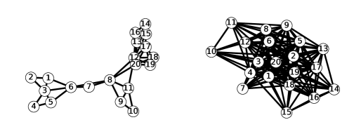
Refer to caption — Figure 1: Networks corresponding to a original sequence (left) and it first-order accumulation sequence (right).

There are two types of explanations of grey accumulation and some important research results [19, 63]. In this subsection, we explain the advantages of grey accumulation by means of complex network theory. We use the data of inbound tourists (10,000 people) downloaded from the National Bureau of Statistics of China (http://www.stats.gov.cn/) for our explanation. Firstly, we convert the original sequence and the first-order accumulation sequence into the form of a complex network respectively.

Definition 1 (See [64])

Suppose $X$ is an original sequence, $X=\left({\boldsymbol{x}_{1}^{(0)},\boldsymbol{x}_{2}^{(0)},\ldots\ldots,\boldsymbol{x}_{n}^{(0)}}\right)$ , and the transformed network is set to ${\rm{G}}=({\rm{V}},{\rm{E}})$ , if $\forall\boldsymbol{x}_{a}^{(0)}$ and $\boldsymbol{x}_{b}^{(0)}$ , $\exists{\rm{\boldsymbol{x}}}_{c}^{(0)}$ , makes

\boldsymbol{x}_{c}^{(0)}<\boldsymbol{x}_{b}^{(0)}+\left({\boldsymbol{x}_{a}^{(0)}-\boldsymbol{x}_{b}^{(0)}}\right)\frac{{{t_{b}}-{t_{c}}}}{{{t_{b}}-{t_{a}}}};({t_{a}}<{t_{c}}<{t_{b}}),

(1)

where $\left({{t_{c}},x_{c}^{(0)}}\right)$ is a point between $\left({{t_{a}},x_{a}^{(0)}}\right)and\left({{t_{b}},x_{b}^{(0)}}\right)$ , then there exists an edge between $x_{a}^{(0)}$ and $x_{b}^{(0)}$ . Through Eq. (1), we can find that if $\left({{t_{c}},x_{c}^{(0)}}\right)$ is the largest number of $\left({{t_{a}},x_{a}^{(0)}}\right)$ and $\left({{t_{b}},x_{b}^{(0)}}\right)$ , then a and b cannot have a link relationship, that is, when there are more fluctuations in the original time series, there will be fewer links in the corresponding network. However, when the first order accumulating generation operator (1?AGO) is employed to preprocess the original data, the sequence is strictly monotonically increasing. As long as $\left({{t_{b}},x_{b}^{(0)}}\right)$ is large enough, there may be a link between $\left({{t_{a}},x_{a}^{(0)}}\right)$ and $\left({{t_{b}},x_{b}^{(0)}}\right)$ . This means that the network formed by the 1-AGO series has more chances to have connections than the original series.

According to Definition 1, we map the time series into a complex network. In Figure 1, we show the complex network after the conversion of the original data and 1-AGO series. We then respectively calculated two types of statistical indicators of the network, namely the clustering coefficient [65] and the average path length [66]. The definition of first-order grey accumulation [1], clustering coefficient, and average path length are as

{x^{(1)}}(k)=\sum\limits_{s=1}^{k}{{x^{(0)}}}(s),...n,C=\frac{1}{n}\sum\limits_{i=1}^{n}{\frac{{2{E_{i}}}}{{{k_{i}}({k_{i}}-1)}}},\frac{1}{{n(n-1)}}{\Sigma_{i\neq j}}{d_{ij}},

(2)

Table 2: The original sequence and the first-order cumulative sequence form a network corresponding to clustering coefficient and average path length.

Data	Clustering coefficient	Average path length
Original sequence	0.708016	2.668421
First-order accumulation	0.856374	1.215789

where $\frac{{2{E_{i}}}}{{{k_{i}}\left({{k_{i}}-1}\right)}}$ is the ratio of the number of edges ${{E_{i}}}$ between the node ${{k_{i}}}$ to the total number of edges. ${d_{ij}}$ refers to the number of edges on the shortest path connecting two nodes, $i$ and $j$ . It can be seen that the 1-AGO series have a larger clustering coefficient and a smaller average path length than the original sequence, so relatively speaking, the 1-AGO series have the characteristics of small-world network [67]. This is mainly because the 1-AGO sequence is more closely connected. In the small-world network, the ability of information dissemination and computing, etc. have been enhanced, that is, the network structure corresponding to the accumulation of the original sequence is compact, which has a stronger efficiency of information dissemination.

2.2 General conformable fractional accumulation and difference

Definition 2 (See [49])

Set that $D_{\psi}^{p}f(u)$ denotes the general conformable derivative of function $f$ , which is defined as

\displaystyle D_{\psi}^{p}f(u)=D_{\psi}^{p-n}{D^{n}}f(u)=\mathop{\lim}\limits_{\epsilon\to 0}\frac{{{f^{(n)}}(u+\epsilon\psi(u,p-n))-{f^{(n)}}(u)}}{\epsilon},

(3)

where $u>0$ , $p\in(n,n+1]$ . Additionally, if $\alpha\in(0,1]$ , Eq. (3) can be changed to

D_{\psi}^{p}f(u)=\mathop{\lim}\limits_{\epsilon\to 0}\frac{{f(u+\epsilon\psi(u,p))-f(u)}}{\epsilon}

(4)

where ${\psi(u,p)}$ is a fractional conformable function [49].

Remark 1

When $\psi(u,p)=1$ , $D_{\psi}^{p}f(u)$ degenerates to the first order derivative case.

Remark 2

When $\psi(u,p)={t^{\left\lceil p\right\rceil-p}}$ and $\alpha\in(n,n+1]$ , $D_{\psi}^{p}f(u)$ is equivalent to the Khalil’s fractional derivative with arbitrary order [48], because of $\psi(u,p)={u^{\left\lceil p\right\rceil-p}}=\psi(u,p-n)={u^{\left\lceil{p-n}\right\rceil-(p-n)}}$ . Specially, when $\psi(u,p)=u^{1-p}$ and $p\in\left({0,1}\right],D_{\psi}^{p}f(u)$ coincides with the Khalil’s fractional derivative [48].

Remark 3

When $q\in(0,1]$ , $\psi(u,p)$ satisfies $\psi(u,1)=1,\psi(\cdot,p)\neq\psi(\cdot,q)$ , where $p\neq q$ . For example, take linear function: $\psi(u,p)=p$ and power function: $\psi(u,p)=p^{2}$ , exponent function: $\psi(u,p)={a^{(1-p)\xi(p)}}$ [49].

Theorem 1 (See [49])

If $f$ is differentiable and ${\rm{}}t>0,p\in(0,1]$ . Then

D_{\psi}^{p}(f)=\frac{{df(u)}}{{du}}\psi(u,p)

(5)

Proof. Set $\xi=\epsilon\psi(u,p)$ , then $\epsilon=\frac{\xi}{{\psi(u,p)}}$ , therefore

\begin{array}[]{l}D_{\psi}^{p}(f)=\mathop{\lim}\limits_{\epsilon\to 0}\frac{{f\left({t+\epsilon\psi(u,p)}\right)-f(t)}}{\epsilon}\\ {\rm{=}}\psi(u,p)\mathop{\lim}\limits_{\xi\to 0}\frac{{f(u+\xi)-f(u)}}{\xi}\\ =\psi(u,p)\frac{{df(u)}}{{du}}\end{array}

(6)

Remark 4

When $p\in\left({n,n+1}\right]$ , $\psi(u,p)\frac{{{d^{n+1}}f(u)}}{{d{u^{n{\rm{+1}}}}}}$ is also established in [49].

According to Definition 2, Theorem 1, and the definition of first-order difference ${\left.{\Delta f(k)\approx\mathop{\lim}\limits_{\xi\to 1}\frac{{f(t)-f(t-\xi)}}{\xi}}\right|_{t=k}}=f(k)-f(k-1)$ [34]. We discretize the first derivative in Eq. (5) into the first difference form, we give the definition of general conformable fractional difference.

Definition 3

The general conformable fractional difference (GCFD) of $f$ with $\alpha$ order is

\begin{array}[]{*{20}{l}}{\Delta^{\alpha}}f(k)=\psi(k,\alpha)\Delta f(k)=\psi(k,\alpha)[f(k)-f(k-1)],\alpha\in(0,1],k\in{N^{+}}\end{array}

(7)

Remark 5

When $\psi(k,\alpha)=1$ , ${\Delta^{\alpha}}f(k)$ degenerates to the first order difference.

Remark 6

When $\psi(k,\alpha)=k^{1-\alpha},{\Delta^{\alpha}}f(k)$ coincides with the Ma’s definition of difference [34].

Remark 7

When $\psi(k,\alpha)=\frac{1}{{{k^{\alpha}}-{{(k-1)}^{\alpha}}}},{\Delta^{\alpha}}f(k)$ coincides with the Yan’s definition of difference [36].

Example 1

Set ${\text{F(k) = (f(1),f(2),f(3)}},{\text{f(4)}},{\text{f(5),f(6)) = (3,7,8}}{\text{.5,12,20,32)}}$ , then

{\Delta^{\alpha}}F(k)={\text{(}}{\Delta^{\alpha}}{\text{f(k))}}=(3,4\psi(2,\alpha),1.5\psi(3,\alpha),3.5\psi(4,\alpha),8\psi(5,\alpha),12\psi(6,\alpha)),k=1,2,...,n.

(8)

As described in [34], integral order difference and accumulation are inverse operations of each other, as shown below,

\begin{array}[]{l}\Delta\nabla f(k)=\Delta\left({\sum\limits_{i=1}^{k}f(i)}\right)=\sum\limits_{i=1}^{k}f(i)-\sum\limits_{i=1}^{k-1}f(i)=f(k)\end{array}

(9)

Inspired by this idea, the GCFD and conformable fractional accumulation (GCFA) should also be inverse operation of each other. It is not difficult to prove that the GCFA and GCFD are inverse operations of each other.

Definition 4

The general conformable fractional accumulative (GCFA) sequence with order $\alpha$ is given by

\begin{array}[]{l}{\nabla^{\alpha}}f(k)=\sum\limits_{i=1}^{k}{\left({\begin{array}[]{*{20}{c}}{k-i+\lceil\alpha\rceil-1}\\ {k-i}\end{array}}\right)}\frac{{f(i)}}{{\psi(i,\alpha)}},\end{array}\alpha\in{R^{+}},k\in{Z^{+}},

(10)

where $\lceil\alpha\rceil$ is the smallest integer greater than or equal to $\alpha$ , $\binom{k-i+\lceil\alpha\rceil-1}{k-i}=\frac{(k-i+\lceil\alpha\rceil-1)!}{(k-i)!(\lceil\alpha\rceil-1)}$ .

Remark 8

When $\psi(i,\alpha)=1$ , GCFA degenerates into a first-order accumulation.

Remark 9

When $\psi(i,\alpha)=\alpha^{i-1}$ , GCFA coincides with Liu’s definition [58].

Remark 10

When $\psi(i,\alpha)={i^{1-\alpha}},\alpha\in\left({0,1}\right],k\in{Z^{+}}$ ,and $\psi(i,\alpha)={i^{\left\lceil\alpha\right\rceil-\alpha}},\alpha\in\left({n,n+1}\right],k\in{Z^{+}}$ , GCFA coincides with Ma’s definition [34]. There is also a unified form of CFA [35].

Remark 11

When $\psi(i,\alpha)={i^{\alpha}}-{(i-1)^{\alpha}}$ , GCFA is equivalent to the definition of Yan (In the text below, we call it FHA) [36].

Remark 12

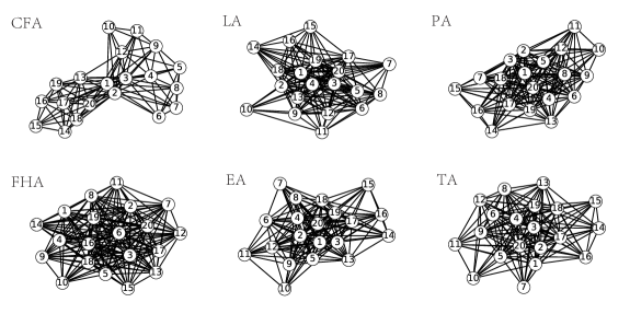
When $\psi(i,\alpha)$ is a linear function or a power function or an exponential function or a trigonometric function, we call it LA, PA, EA or TA. In short, as long as a meets the requirements in Remark 3, it is valid.

We calculate the clustering coefficients and the average length of different accumulations. We choose $\psi(i,\alpha)$ = $\alpha$ for LA, $\psi(i,\alpha)$ = ${\alpha^{2}}$ for PA, $\psi(i,\alpha)$ = ${2^{1-\alpha}}$ for EA and $\psi(i,\alpha)$ , $\sin\left({\frac{\pi}{2}\alpha}\right)$ for TA with order of 0.9. The statistical indicators of several types of accumulation are listed in the Table 3, data from Subsection 2.1. We can see that in this example, the clustering system of FHA is the largest one with a value of 0.933576, and the clustering coefficient of CFA is the smallest, which is 0.782559. They are both greater than the clustering coefficient of the original sequence: 0.708016. The average path length of FHA is the smallest one with 1.08421, and the average path length of CFA is the largest with 1.473684. The network structure formed by different accumulations is illustrated in Figure 2. It can be seen that their structure are different. Further, compared to the original sequence, their structure is more compact.

Table 3: Clustering coefficient and average path length of different fractional accumulation forms with order is 0.9.

Data	CFA	LA	PA	EA	TA	FHA
Clustering coefficient	0.782559	0.856374	0.856374	0.856374	0.856374	0.933576
Average path length	1.473684	1.215789	1.215789	1.215789	1.215789	1.08421

3 Generalized conformable fractional grey model

In this section, we propose a new grey prediction model based on GCFA and GCFD operators.

3.1 Basic definition of generalized conformable fractional grey model

Definition 5

With the data sequence ${\bf{{X}}}_{n\times 1}^{(0)}={\left({{{x}^{(0)}}(1),{{x}^{(0)}}(2),\ldots,{{x}^{(0)}}(n)}\right)^{T}}$ , GCFA can be given by ${\bf{{X}}}_{{\rm{n}}\times 1}^{(\alpha)}={\left({{{x}^{(\alpha)}}(1),{{x}^{(\alpha)}}(2),\ldots,{{x}^{(\alpha)}}(n)}\right)^{T}}$ , where

{{x}^{(\alpha)}}(k)={\nabla^{\alpha}}{{x}^{(0)}}(k)=\sum\limits_{i=1}^{k}{\left({\begin{array}[]{*{20}{c}}{k-i+\lceil\alpha\rceil-1}\\ {k-i}\end{array}}\right)}\frac{{{x}(i)}}{{\psi(i,\alpha)}},k=1,2,3,...,n.

(11)

We represent the $p$ -order ( $p\in\left({0,1}\right]$ )differential equation of general conformable fractional grey model GCFGM(1,1) wirth the $\alpha$ -GCFA (Eq. (10)) series as

\displaystyle D_{\psi}^{p}{{x}^{(\alpha)}}(t)+{a}{{x}^{(\alpha)}}(t)={b}.

(12)

Obviously, when $p=1$ and $\alpha=1$ , the model degenerates to GM(1,1) [1]. In the actual modeling environment, the appropriate accumulation method should be selected according to the actual background of data. In particular, the accumulation can be also choosed the weighted form of two functions, such as

\displaystyle{\nabla^{\alpha}}{{x}^{(0)}}(k)=\sum\limits_{i=1}^{k}{\left({\begin{array}[]{*{20}{c}}{k-i+\lceil\alpha\rceil-1}\\ {k-i}\end{array}}\right)}\frac{{{x}(i)}}{{\frac{1}{2}\left({{\alpha^{i-1}}{\rm{+}}{i^{1-\alpha}}}\right)}},k=1,2,3,...,n.

(15)

Theorem 2

The exact solution to Eq. (12) is

\displaystyle{x^{(\alpha)}}(t)={{\rm{e}}^{-\int{\frac{a}{{\psi(t,p)}}}{\rm{dx}}}}\left({\int{\frac{b}{{\psi(t,p)}}}{{\rm{e}}^{\smallint\frac{a}{{\psi(t,p)}}{\rm{dx}}}}{\rm{dx}}+{\rm{C}}}\right).

(16)

Proof. Using Eq. (6), Eq. (12) can be arranged as

\displaystyle\psi(t,p)\frac{{{\rm{d}}{x^{(\alpha)}}(t)}}{{{\rm{d}}t}}+a{x^{(\alpha)}}(t)=b.

(17)

Set ${x^{(\alpha)}}(x)=C(x)\cdot{e^{-\int{\frac{a}{{\psi(t,p)}}}dx}}$ , we have

\displaystyle\frac{{d{x^{(\alpha)}}(x)}}{{dx}}=\frac{{dC(x)}}{{dx}}{e^{-\int{\frac{a}{{\psi(t,p)}}}dx}}-{x^{(\alpha)}}(x)\frac{a}{{\psi(t,p)}}.

(18)

Based on Eq. (17), we have

\displaystyle\frac{{d{x^{(\alpha)}}(x)}}{{dx}}=\frac{b}{{\psi(t,p)}}-\frac{a}{{\psi(t,p)}}{x^{(\alpha)}}(x).

(19)

Combining Eq. (12) and Eq. (19), we have

\displaystyle\frac{{dC(x)}}{{dx}}={e^{\int{\frac{a}{{\psi(t,p)}}}dx}}\frac{b}{{\psi(t,p)}},C\left(x\right)=\int{\frac{b}{{\psi(t,p)}}}{e^{\smallint\frac{a}{{\psi(t,p)}}dx}}dx+{C_{1}}.

(20)

Substitite Eq. (20) into ${x^{(\alpha)}}(x)=C(x)\cdot{e^{-\int{\frac{a}{{\psi(t,p)}}dx}}}$ , we can get Eq. (16). Set ${x^{(\alpha)}}(1)={x^{(0)}}(1)$ , we can get the time response sequence of GCFGM(1,1)by Theorem 2 as

\displaystyle{x^{(\alpha)}}(t)={{\rm{e}}^{-\int{\frac{a}{{\psi(t,p)}}}{\rm{d}}x}}\left({\int{\frac{b}{{\psi(t,p)}}}{{\rm{e}}^{\int{\frac{a}{{\psi(t,p)}}{\rm{dx}}}}}{\rm{dx}}+\frac{{{x^{(0)}}(1)}}{{{{\rm{e}}^{-\int{\frac{a}{{\psi(t,p)}}}{\rm{d}}x}}}}-\int{\frac{b}{{\psi(t,p)}}}{{\rm{e}}^{\int{\frac{a}{{\psi(t,p)}}{\rm{dx}}}}}{\rm{dx}}}\right).

(21)

In order to estimate the parameters $[\hat{a},\hat{b}]^{T}$ in GCFM(1,1), we need to discretize Eq. (12). Integrating both sides of Eq. (12) with $p$ order, we have

\displaystyle\iint\cdots\int_{k-1}^{k}{\frac{{{d^{p}}{x^{(\alpha)}}}}{{d{t^{p}}}}}d{t^{p}}+a\iint\cdots\int_{k-1}^{k}{{x^{(\alpha)}}}(t)d{t^{p}}=b\iint\cdots\int_{k-1}^{k}d{t^{p}}.

(22)

Taking the p-th order integral on $\frac{{{d^{p}}{x^{(\alpha)}}(t)}}{{d{t^{p}}}}d{t^{p}}$ , we can get

\displaystyle\iint\cdots\int_{k-1}^{k}{\frac{{{d^{p}}{x^{(\alpha)}}(t)}}{{d{t^{p}}}}}d{t^{p}}\approx\Delta^{p}x^{(\alpha)}(k)={x^{(\alpha-p)}}(k).

(23)

Using the general trapezoid formula [73], we can get

\displaystyle a\iint\cdots\int_{k-1}^{k}{{x^{(\alpha)}}}(t)d{t^{r}}\approx\frac{a}{{\rm{2}}}\left({{x^{(\alpha)}}(k-1)+{x^{(\alpha)}}(k)}\right).

(24)

The right-hand side of Eq. (12) can be obtained by Ref. [73], as

\displaystyle\iint\cdots\int_{k-1}^{k}bd{t^{r}}=b\iint\cdots\int_{k-1}^{k}d{t^{r}}\approx\int_{k-1}^{k}{bd}t\approx b.

(25)

Substituting Eqs. (23)-(25) into Eq. (22), We can get the discrete form of the GCFGM model as follows,

\displaystyle{{x}^{(\alpha-p)}}(k)+\frac{{a}}{2}\left({{{x}^{(\alpha)}}(k)+{{x}^{(\alpha)}}(k-1)}\right)={{b}},k=1,2,3,...,n.

(26)

As we know, the differential equations and corresponding difference equations of the classic GM(1,1) model are as follows,

\displaystyle\frac{{d{{x}^{(1)}}(t)}}{{dt}}+{a}{{x}^{(1)}}(t)={b},{{x}^{(0)}}(k)+\frac{{a}}{2}\left({{{x}^{(1)}}(k)+{{x}^{(1)}}(k-1)}\right)={b},k=1,2,3,...,n.

(27)

It is well known that $\frac{{d{x^{(1)}}(t)}}{{dt}}$ is an continuous representation of ${x^{(0)}}(k)={x^{(1)}}(k)-{x^{(1)}}(k-1)$ . Therefore, the effect of the first-order derivative can be approximately regarded as a bridge from the first-order cumulative generated sequence to the original sequence. The physical meaning of the classical first derivative is very clear, which means velocity of particle or slope of a tangent respectively [49]. But due to the uncertainty and complexity of the real world, in the grey system, the change from the first-order cumulative sequence to the original sequence does not necessarily satisfy the law of classical derivatives. Zhao and Luo [49] gave the physical meaning of the general conformable fractional derivative: GCFD is a modification of classical derivative in direction and magnitude. Therefore, in the grey system model, we use GCFD for modeling real world system, which represents a special change from the first-order cumulative sequence to the original sequence. The parameters of the GCFGM model can be obtained by the least squares method. Set ${z^{(\alpha)}}(k+1)=\frac{{{x^{(\alpha)}}(k)+{x^{(\alpha)}}(k+1)}}{2},k=1,2,\cdots,n-1$ , we have

\displaystyle[\hat{a},\hat{b}]=\mathop{\arg\min}\limits_{a,b}\left\{{\sum\limits_{i=1}^{n-1}{{{\left[{{x^{(\alpha-p)}}(k)-\left({-a\cdot{z^{(\alpha)}}(k+1)+b}\right)}\right]}^{2}}}}\right\}={\left({{B^{T}}B}\right)^{-1}}{B^{T}}Y,

(28)

where

B=\left({\begin{array}[]{*{20}{c}}{-{z^{(\alpha)}}(2)}&1\\ {-{z^{(\alpha)}}(3)}&1\\ \vdots&\vdots\\ {-{z^{(\alpha)}}(n)}&1\end{array}}\right),Y=\left({\begin{array}[]{*{20}{c}}{{x^{(\alpha-p)}}(2)}\\ {{x^{(\alpha-p)}}(3)}\\ \vdots\\ {{x^{(\alpha-p)}}(n)}\end{array}}\right).

Using the definition of GCFD, the restored values can be written

\displaystyle{{{\hat{x}}^{(0)}}(k)=\psi(k,\alpha)\left({{{\hat{x}}^{(\alpha)}}(k)-{{\hat{x}}^{(\alpha)}}(k-1)}\right).k=2,3,\ldots,n.}

(29)

Through the model established above, we can get the result of GCFGM $\widehat{X}^{(0)}$ . In the above analysis, we assume that the order of the model $p$ and $\alpha$ are already known. But in practice, the parameters should be dynamically adjusted according to the actual data. In order to better understand the modeling process of GCFGM, the modeling steps of GCFGM with given time series and $\alpha$ and p can be summarized as follows:

$\boldsymbol{Step\ 1:}$ Calculate the $\alpha$ order GCFA sequences $\left({{x^{(\alpha)}}(1),{x^{(\alpha)}}(2),\ldots,}\right.\left.{{x^{(\alpha)}}(n)}\right)$ of the raw series

$\left(\chi^{(0)}(1),x^{(0)}(2),\ldots,x^{(0)}(n)\right)$ ;

$\boldsymbol{Step\ 2:}$ Calculate the parameters of GCFGM $\hat{a}$ and $\hat{b}$ by Eq. (28)

$\boldsymbol{Step\ 3:}$ Calculate the predicted values of the GCFA series using Eq. (21);

$\boldsymbol{Step\ 4:}$ Calculate the restored values of the GCFD series $\hat{x}^{(0)}(k),k=1,2,3,..,n+u$ using Eq. (21), where n is the number of samples for building model and u is the number of prediction steps;

3.2 Intelligent optimization algorithm for selecting the optimal p and $\alpha$

In the above analysis, we assume that the order of GCFM is known. So, in order to get the appropriate order, we can design the following model,

\displaystyle{\min_{\alpha,p},}{\text{MAPE }}=\sum\limits_{i=1}^{\text{n}}{\left|{\frac{{{{\hat{x}}^{(0)}}(i)-{x^{(0)}}(i)}}{{{x^{(0)}}(i)}}}\right|}\times 100\%,{\text{ s}}{\text{.t}}{\text{. }}\left\{\begin{gathered}{\color[rgb]{0,0,1}Eq}.(\ref{GCFA})\hfill\\ {\color[rgb]{0,0,1}Eq}.(\ref{para1})\hfill\\ {\color[rgb]{0,0,1}Eq}.(\ref{trespose1})\hfill\\ {\color[rgb]{0,0,1}Eq}.(\ref{GCFD})\hfill\\ \end{gathered}\right..

(35)

In order to get an appropriate order, combined with the above model, We first consider using PSO[72] search for the order of GCFM model respectively, which are widely used in engineering and science, and have achieved good performance. The concrete algorithm for searching order of model is presented in Algorithm 1.

Input: Raw data

X^{(0)}=\left\{x^{(0)}(1),x^{(0)}(2),\ldots,x^{(0)}(n)\right\}

Output: Optimized fractional order

\ \alpha,p

1 Set the maximum iteration number and maximum population

2Initialize Particle swarm

3Initialize velocity and position

4for $t\leftarrow 1;t<{\text{max iteration number}};{\text{t}}\leftarrow{\text{t + 1}}$ do

5 for $j\leftarrow 1;j<{\text{maximum population}};{\text{j}}\leftarrow{\text{j + 1}}$ do

6 Update the velocity and position

7 Construct

\alpha

-GCFA series of

X^{(0)}

using Eq.(11)

8 Get the parameters of the model

[\hat{a},\hat{b}]

using Eq.(28)

9 Compute

\hat{X}^{(r)}(k)

by time response function of GCFGM using Eq.(21)

10 Compute restored values

\hat{x}^{(0)}(k)

using Eq.(29)

11 Compute fitness using Eq.(35)

Return the optimized order

\alpha

Algorithm 1 Particle swarm optimization to search the fractional order

\alpha

and

p

of GCFGM

3.3 Properties of the GCFGM model

Wu et al. [33] first discusses the information priority in grey model prediction with matrix perturbation bound theory, which is the basis of grey modeling. In this subsection, we will use this technique to analyze the characteristics of GCFGM.

Lemma 1 (See [74])

Set $A\in{C^{m\times n}},b\in{C^{m}},{A^{\eta}}$ is the generalized inverse matrix of $\text{ A, }B=A+W\text{ and }c=b+k\in C^{m}$ . Then $x$ and $x+h$ satisfy $\|Ax-b\|_{2}=\min\text{ and }\|Bx-c\|_{2}=\min$ . If $\operatorname{rank}(A)=\operatorname{rank}(B)=n{\text{ and }}{\left\|{{A^{\dagger}}}\right\|_{2}}W{{}_{2}}<1$ , then

\displaystyle\|h\|\leq\frac{\kappa_{\dagger}}{\gamma_{\dagger}}\left(\frac{\|W\|_{2}}{\|A\|}\|x\|+\frac{\|k\|_{2}}{\|A\|}+\frac{\kappa_{\dagger}}{\gamma_{\dagger}}\frac{\|W\|_{2}}{\|A\|}\frac{\left\|r_{x}\right\|}{\|A\|}\right),

(36)

where $\kappa_{\dagger}=\left\|A^{\dagger}\right\|_{2}\|A\|,\gamma_{\dagger}=1-\left\|A^{\dagger}\right\|_{2}\|W\|_{2},r_{x}=b-Ax$ .

Theorem 3

Set $p=1$ , we can get the following differential equation $D_{\psi}^{1}x^{(\alpha)}(t)+ax^{(\alpha)}(t)=b$ , the corresponding difference equation is ${x^{(\alpha-1)}}(k)+\frac{a}{2}\left({{x^{(\alpha)}}(k)+{x^{(\alpha)}}(k-1)}\right)=b,k=1,2,3,\ldots,n$ , where $D_{\psi}^{1}x^{(\alpha)}(t)$ is equivalent to classic first derivative. Set $x$ is the solution of the GCFGM model, which satisfies $\min\|Bx-Y\|_{2}$ . if $\varepsilon$ is a disturbance of original value $x^{(0)}(k)(k=1,2,\cdots n)$ , the perturbation bound of the $x$ is

\displaystyle L\left[x^{(0)}(1)\right]=\left|\frac{\varepsilon}{\psi(1,\alpha)}\right|\frac{\kappa_{\dagger}}{\gamma_{\dagger}}\left(\frac{\sqrt{n-1}}{\|B\|}\|x\|+\frac{\kappa_{\dagger}}{\gamma_{\dagger}}\frac{\sqrt{n-1}}{\|B\|}\frac{\left\|r_{x}\right\|}{\|B\|}\right){\text{, k = 1}}.

(37)

\displaystyle L\left[x^{(0)}(k)\right]=\left|\frac{\varepsilon}{\psi(k,\alpha)}\right|\frac{\kappa_{\dagger}}{\gamma_{\dagger}}\left(\frac{\sqrt{n-k+\frac{1}{4}}}{\|B\|}\|x\|+\frac{1}{\|B\|}+\frac{\kappa_{\dagger}}{\gamma_{\dagger}}\frac{\sqrt{n-k+\frac{1}{4}}}{\|B\|}\frac{\left\|r_{x}\right\|}{\|B\|}\right),k=2,3,\cdots,n.

(38)

Proof. if $\varepsilon$ is regarded as a disturbance of $x^{(0)}(1)$ , the subsequent is working,

\displaystyle Y+\Delta Y=\left({\begin{array}[]{*{20}{c}}{\frac{{{x^{(0)}}(2)}}{{\psi(2,\alpha)}}}\\ {\frac{{{x^{(0)}}(3)}}{{\psi(3,\alpha)}}}\\ \vdots\\ {\frac{{{x^{(0)}}(n)}}{{\psi(n,\alpha)}}}\end{array}}\right)+\left({\begin{array}[]{*{20}{c}}0\\ 0\\ \vdots\\ 0\end{array}}\right),B+\Delta B={\text{B + }}\left({\begin{array}[]{*{20}{c}}{-\frac{\varepsilon}{{\psi(1,\alpha)}}}&0\\ {-\frac{\varepsilon}{{\psi(1,\alpha)}}}&0\\ \vdots&\vdots\\ {-\frac{\varepsilon}{{\psi(1,\alpha)}}}&0\end{array}}\right).

(51)

Therefore, $\|\Delta Y\|_{2}=0,\|\Delta B\|_{2}=\sqrt{n-1}\left|\frac{\varepsilon}{\psi(1,r)}\right|$ ,so the the perturbation bound can be defined as

\displaystyle\|\Delta x\|\leq\frac{\kappa_{\dagger}}{\gamma_{\dagger}}\left(\frac{\|\Delta B\|_{2}}{\|B\|}\|x\|+\frac{\|\Delta Y\|_{2}}{\|B\|}+\frac{\kappa_{\dagger}}{\gamma_{\dagger}}\frac{\|\Delta B\|_{2}}{\|B\|}\frac{\left\|r_{x}\right\|}{\|B\|}\right).

(52)

So, Eq. (37) is proved. If $\varepsilon$ is regarded as a disturbance of $x^{(0)}(2)$ , then

\displaystyle Y+\Delta Y=\left({\begin{array}[]{*{20}{c}}{\frac{{{x^{(0)}}(2)}}{{\psi(2,\alpha)}}}\\ {\frac{{{x^{(0)}}(3)}}{{\psi(3,\alpha)}}}\\ \vdots\\ {\frac{{{x^{(0)}}(n)}}{{\psi(n,\alpha)}}}\end{array}}\right)+\left({\begin{array}[]{*{20}{c}}{\frac{\varepsilon}{{\psi(2,\alpha)}}}\\ 0\\ \vdots\\ 0\end{array}}\right)B+\Delta B=B{\text{ + }}\left({\begin{array}[]{*{20}{c}}{-\frac{\varepsilon}{{2\psi(2,\alpha)}}}&0\\ {-\frac{\varepsilon}{{\psi(2,\alpha)}}}&0\\ \vdots&\vdots\\ {-\frac{\varepsilon}{{\psi(2,\alpha)}}}&0\end{array}}\right).

(65)

The perturbation bound can be expressed as

\displaystyle L\left[x^{(0)}(2)\right]=\left|\frac{\varepsilon}{\psi(2,r)}\right|\frac{\kappa_{\dagger}}{\gamma_{\dagger}}\left(\frac{\sqrt{n-\frac{7}{4}}}{\|B\|}\|x\|+\frac{1}{\|B\|}+\frac{\kappa_{\dagger}}{\gamma_{\dagger}}\frac{\sqrt{n-\frac{7}{4}}}{\|B\|}\frac{\left\|r_{x}\right\|}{\|B\|}\right).

(66)

If $\varepsilon$ is regarded as a disturbance of $x^{(0)}(n)$ , we can get

\displaystyle L\left[x^{(0)}(n)\right]=\left|\frac{\varepsilon}{\psi(n,r)}\right|\frac{\kappa_{\dagger}}{\gamma_{\dagger}}\left(\frac{1}{2\|B\|}\|x\|+\frac{1}{\|B\|}+\frac{\kappa_{\dagger}}{\gamma_{\dagger}}\frac{1}{2\|B\|}\frac{\left\|r_{x}\right\|}{\|B\|}\right).

(67)

Without loss of generality, when $k=2,3,\cdots,n$ , we can easily obtain Eq. (38) using the same method as above.

In the above analysis, we use perturbation boundary theory to prove the stability of the GCFGM(1,1) model with different disturbed raw data. Through Theorem 3, the following conclusion is working, the sample size $n$ is an increase function of $L\left[{{x^{(0)}}(k)}\right]k=1,2,3,...,n$ . Therefore, in order to increase the stability of GCFGM model, we should use less data in actual modeling background. In the following study, we will explore the influence of initial value on GCFGM(1,1).

Theorem 4

Set $X^{(0)}=\left\{x^{(0)}(1),x^{(0)}(2),\cdots,x^{(0)}(n)\right\}$ is the raw nonnegative data. if $\varepsilon$ is regarded as a disturbance of $x^{(0)}(1)$ and $\psi({\text{1}},\alpha){\text{ = 1}}$ . $x^{(0)}(1)+\varepsilon$ dose not cause the changing of GCFGM’s simulative value $\hat{X}^{(0)}=\left\{\hat{x}^{(0)}(2),\cdots,\hat{x}^{(0)}(n),\hat{x}^{(0)}(n+1),\cdots\right\}$ .

Proof. When ${x^{(0)}}(1)+\varepsilon$ exists, we have $X^{(\alpha)}+\varepsilon=\left\{x^{(0)}(1)+\varepsilon,x^{(\alpha)}(2)+\varepsilon,\cdots,x^{(\alpha)}(n)+\varepsilon\right\}$ . The complete proof process is similar to Theorem 1 of Reference [75]. In order to verify the validity of this conclusion, we furniture our results by illustrative numerical examples for the GCFGM (Sets 1 is the electricity consumption of Jiangsu province in China published by China s National Statistics Bureau (http://www.stats.gov.cn/english/)) and choose Eq. (15) as the accumulation of GCFM.

Table 4: The simulation results of GCFGM with different initial values

Sets 1	Sets 2	Model 1	APE(%)	Model 2	APE(%)	Model 3	APE(%)	Model 4	APE(%)
971.34	1071.34	971.34	0.00	1071.34	0.00	971.34	0.00	1071.34	0.00
1078.44	1078.44	1431.75	32.76	1431.75	32.76	918.4131	14.84	918.4131	14.84
1245.14	1245.14	1542.83	23.91	1542.83	23.91	1253.323	0.66	1253.323	0.66
1505.13	1505.13	1721.41	14.37	1721.41	14.37	1609.24	6.92	1609.24	6.92
1820.08	1820.08	1937.80	6.47	1937.80	6.47	1955.808	7.46	1955.808	7.46
2193.45	2193.45	2176.49	0.77	2176.49	0.77	2291.823	4.48	2291.823	4.48
2569.75	2569.75	2429.99	5.44	2429.99	5.44	2618.384	1.89	2618.384	1.89
2952.02	2952.02	2695.04	8.71	2695.04	8.71	2936.48	0.53	2936.48	0.53
3118.32	3118.32	2970.53	4.74	2970.53	4.74	3246.873	4.12	3246.873	4.12
3313.99	3313.99	3256.41	1.74	3256.41	1.74	3550.162	7.13	3550.162	7.13
3864.37	3864.37	3553.20	8.05	3553.20	8.05	3846.826	0.45	3846.826	0.45
4281.62	4281.62	3861.63	9.81	3861.63	9.81	4137.264	3.37	4137.264	3.37
4580.90	4580.90	4182.58	8.70	4182.58	8.70	4421.811	3.47	4421.811	3.47
4956.60	4956.60	4516.95	8.87	4516.95	8.87	4700.753	5.16	4700.753	5.16
5012.54	5012.54	4865.69	2.93	4865.69	2.93	4974.338	0.76	4974.338	0.76
5114.70	5114.70	5229.73	2.25	5229.73	2.25	5242.787	2.50	5242.787	2.50
5458.95	5458.95	5610.04	2.77	5610.04	2.77	5506.292	0.87	5506.292	0.87
5807.89	5807.89	6007.60	3.44	6007.60	3.44	5765.029	0.74	5765.029	0.74
6128.27	6128.27	6423.40	4.82	6423.40	4.82	6019.155	1.78	6019.155	1.78
6264.36	6264.36	6858.47	9.48	6858.47	9.48	6268.813	0.07	6268.813	0.07
MAPE(%)			8.42		8.42		3.54		3.54

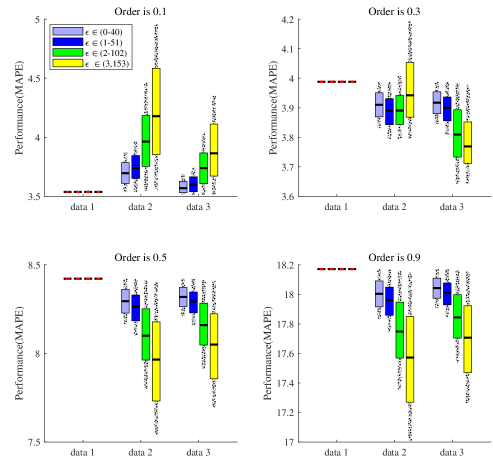
From Table 4, we can easily see that although the initial value has changed under the action of different orders, the simulated value of GCFGM has not changed. The initial value of Sets 2 is different from of Sets 1, and other data are consistent. Model 1 and Model 3 are different models built with Sets 1, their cumulative orders are 0.5 and 0.1 respectively. Model 2 and Model 4 are different models built with Sets 2, and their cumulative orders are 0.5 and 0.1 respectively. In order to further describe the influence of different orders and different initial values on fitting results of GCFM, four cumulative orders and different initial values can be employed to observe the fitting results of the raw samples. We change first three values of the model ( ${x^{(0)}}(1),{x^{(0)}}(2),{x^{(0)}}(3)$ ) into disturbance values ( $x^{(0)}(1)+\epsilon,x^{(0)}(2)+\epsilon,x^{(0)}(3)+\epsilon$ ) in four different intervals , and generate 500 disturbance values in each interval with different $\epsilon$ . By substituting different disturbance values into GCFM, different fitting errors are obtained. It can be seen from Figure 3, Under the influence of different cumulative order and disturbance intensity, the change of initial value do not affect the fitting values of the model, while the change of second value and the third value will directly affect the fitting results of the model.

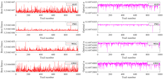
In this numerical example, the another aim is to compare the performances of the (WOA[69], ALO[70], GWO[71], PSO). we use the four algorithms to search the minimum MAPE and the corresponding order $\alpha$ of the GCFGM(1,1) model among the 1000 trails. The optimal orders of th e model and MAPE in each trail are presented in textcolorblueFig. 4. It can be seen clearly in textcolorblueFig. 4that PSO is more stable than the other three optimizer. According to the above analysis, the PSO should be employed to construct GCFGM(1,1) model in the engineering application when we need more stable output of the model.

4 Application

In this section, we use the GCFGM(1,1) model to evaluate China’s total energy consumption (10,000 tons of standard coal) and natural gas consumption (10,000 tons of standard coal) (data sets were published by China’s National Statistics Bureau (http://www.stats.gov.cn/english/)). For simple consideration, we choose the order of the differential equation as 1. In order to comprehensively utilize the characteristics of different accumulations, we choose Eq. (15) as the fractional accumulation. To verify the effectiveness of the proposed model, we use several other representative models (CFGM(1,1)[34], GM(1,1)[14], DGM(1,1)[21]) to compare with our GCFGM(1,1). We use MAPE as the evaluation standard of the model, and their definitions is

\displaystyle\operatorname{APE}(k)=\left|{\frac{{{x^{(0)}}(k)-{{\hat{x}}^{(0)}}(k)}}{{{x^{(0)}}(k)}}}\right|\times 100\%,k=2,3,\ldots,n

(68)

\displaystyle\text{MAPE}=\frac{1}{n}\sum_{i=1}^{n}\frac{\left|\widehat{x}^{(0)}(k)-x^{(0)}(k)\right|}{x^{(0)}(k)}\times 100\%

(69)

and choose Eq. (15) as the accumulation of GCFM. Compared with PSO, although the other three algorithms (PSO, ALO, GWO,) have been proved to have excellent characteristics, they have also been widely applied to complex problems in various fields. But our problem is relatively simple, we only need to search for one parameter. Through the above analysis, we found that PSO has better stability. Here we consider more about the stability of GCFGM(1,1), so in the stage of application, we consider using PSO algorithm.

Case 1. In this case, we use four models, (GCFGM(1,1), CFGM, GM(1,1), DGM(1,1)), to predict China’s overall energy consumption. The data from 2010 to 2015 are used as the training samples to build the models, and the data from 2016 to 2019 are used as the test samples. Finally, we calculate MAPEs of the models on the training set and the test set. The results can be seen in Table 5 and Figure 5.

Table 5: Numerical results by GCFGM(1,1), CFGM(1,1), GM(1,1), DGM(1,1) in Case 1.

Year	True value	GCFGM(1,1)	Error(%)	CFGM(1,1)	Error(%)	GM(1,1)	Error(%)	DGM(1,1)	Error(%)
2000	146964.00	146964	0	146964	0	146964	0	146964	0
2001	155547.00	153215	1.499193	143444.7	7.780508	194808.3	25.24076	195148.2	25.45932
2002	169577.00	174011.2	2.614887	178497.3	5.260306	207586.3	22.41416	207923.5	22.61303
2003	197083.00	201730.1	2.357929	208504.8	5.79542	221202.4	12.23821	221535.1	12.40701
2004	230281.00	229724.2	0.241785	235262.4	2.163162	235711.7	2.358297	236037.8	2.499905
2005	261369.00	256213	1.972672	259699.2	0.638866	251172.7	3.901114	251489.9	3.779747
2006	286467.00	280880.3	1.950208	282371.2	1.429771	267647.8	6.569408	267953.6	6.462668
2007	311442.00	303812.4	2.449779	303642.4	2.504345	285203.6	8.424818	285495	8.33123
2008	320611.00	325179.9	1.425075	323767	0.984368	303910.9	5.208843	304184.9	5.123388
2009	336126.00	345150	2.684719	342930.6	2.024413	323845.2	3.653619	324098.2	3.578366
2010	360648.00	363866.5	0.892424	361273.8	0.173524	345087.1	4.314693	345315.1	4.25148
2011	387043.00	381449.8	1.445117	378906.2	2.102287	367722.4	4.991855	367921	4.940531
2012	402138.00	398000.6	1.028843	395915.2	1.547422	391842.3	2.560238	392006.8	2.519333
2013	416913.00	413604.2	0.793635	412371.7	1.089261	417544.3	0.151431	417669.4	0.181418
2014	428333.99	428333.4	0.000135	428334.4	8.42E-05	444932.2	3.87507	445011.9	3.893668
2015	434112.78	442251.2	1.874714	443852.2	2.243512	474116.6	9.21507	474144.4	9.221478
MAPE			1.548741		2.382483		7.674506		7.684171
2016	441491.81	455412.5	3.153109	458966.7	3.958146	505215.2	14.43365	505184	14.4266
2017	455826.92	467866.1	2.64118	473713.6	3.924001	538353.7	18.10484	538255.7	18.08335
2018	471925.15	479655.2	1.637983	488123.5	3.4324	573665.8	21.55864	573492.4	21.52189
2019	487000.00	490818.5	0.784089	502223.3	3.12593	611294.1	25.52241	611035.8	25.46936
MAPE			2.05409		3.610119		19.90489		19.8753

Table 6: The fitness (MAPE) and order searched by the PSO algorithms in Case 1.

	PSO-GCFGM	PSO-CFGM
Order	0.3228	0.4631
MAPE	1.5487	2.3825

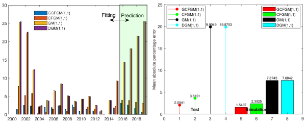
It can be seen from Table 5 that in fitting stage, MAPEs of GCFGM(1,1), CFGM(1,1), GM(1,1) and DGM(1,1) are 1.548741%, 2.382483%, 7.674506% and 7.684171%, respectively. In prediction stage, MAPEs are 1.548741%, 2.382483%, 7.674506%, 7.684171%, respectively. It can be found that the error of GCFGM(1,1) is the smallest one in both fitting stage and prediction stage. This verifies that GCFGM(1,1) has certain advantages. The fitness (MAPE) and order searched by the PSO algorithm are shown in Table 6, we can see that after the optimization of PSO, the order of GCFGM (1,1) model is 0.3228, and the corresponding MAPE is 1.5487. The order of CFGM(1,1) model is 0.4631, and the corresponding MAPE is 2.3825.

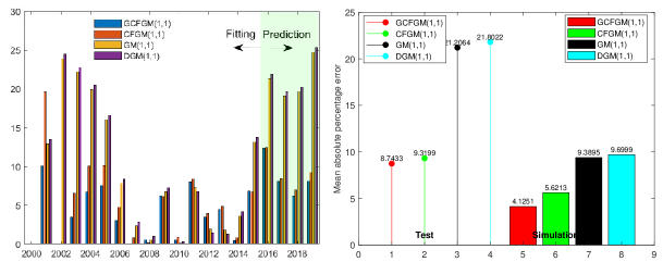
Case 2. Forecasting China’s natural gas consumption. The prediction of natural gas is of great significance and can provide important suggestions to decision makers. In this Case, we use the model to fit China’s natural gas consumption data from 2000 to 2015 and the data from 2016 to 2019 to test the established model, and calculate MAPE of the fitting and predicting stages respectively. It can be found from Tabel 7 that in fitting stage, MAPEs of GCFGM(1,1), CFGM(1,1), GM(1,1), DGM(1,1) are 4.125082%, 5.621349%, 9.389527%, 9.699885% respectively. The MAPE in prediction phase is 8.7433%, 9.319867%, 21.20638%, 21.80221%. It can be seen from Tabel 7 that in this case, compared with the other three models, the output of GCFGM is closest to the real value regardless of the fitting order and the prediction stage. Like Case 1, The fitness (MAPE) and order searched by the PSO algorithm are shown in Table 8, we can see that after the optimization of PSO, the order of GCFGM(1,1) model is 0.4382, and the corresponding MAPE is 4.1251. The order of CFGM(1,1) model is 0.58628, and the corresponding MAPE is 5.6213.

From these two cases, we can see that it is possible to improve the fitting and prediction accuracy of the model by reconstructing the grey prediction model with GCFA and GCFD. In practical modeling problems, we can flexibly adjust our accumulation types of accumulation according to the establishment principles of GCFA and GCFD when the higher accuracy is needed in fitting and forecasting.

Table 7: Numerical results by GCFGM(1,1), CFGM(1,1), GM(1,1), DGM(1,1) in Case 2.

Year	True value	GCFGM(1,1)	Error(%)	CFGM	Error(%)	GM(1,1)	Error(%)	DGM(1,1)	Error(%)
2000	3233.21	3233.21	0	3233.21	0	3233.21	0	3233.21	0
2001	3733.13	3356.357	10.09268	2998.57	19.67679	4217.306	12.9697	4237.064	13.49897
2002	3900.27	3900.32	0.001285	3900.292	0.000564	4834.06	23.94168	4856.776	24.52409
2003	4532.91	4691.734	3.503796	4831.9	6.59599	5541.011	22.2396	5567.126	22.81572
2004	5296.46	5651.381	6.701094	5828.317	10.04174	6351.349	19.91688	6381.372	20.48372
2005	6272.86	6747.777	7.570974	6912.479	10.1966	7280.194	16.05861	7314.71	16.60884
2006	7734.61	7973.455	3.087998	8103.32	4.767016	8344.877	7.890084	8384.557	8.403095
2007	9343.26	9332.969	0.110147	9418.625	0.806625	9565.263	2.376079	9610.879	2.864302
2008	10900.77	10837.15	0.583623	10876.33	0.224174	10964.12	0.58118	11016.56	1.062248
2009	11764.41	12500.46	6.256613	12495.27	6.212442	12567.56	6.826925	12627.84	7.339358
2010	14425.92	14339.85	0.596613	14295.61	0.903272	14405.48	0.141662	14474.79	0.33874
2011	17803.98	16374.31	8.030042	16299.3	8.451343	16512.2	7.255592	16591.86	6.808119
2012	19302.62	18624.79	3.511579	18530.33	4.000938	18927	1.945948	19018.58	1.471486
2013	22096.39	21114.28	4.444682	21015.08	4.893586	21694.96	1.816739	21800.24	1.340279
2014	23986.7	23867.93	0.49514	23782.64	0.850741	24867.71	3.672901	24988.73	4.177449
2015	25178.54	26913.33	6.889961	26865.1	6.698415	28504.45	13.20932	28643.58	13.76186
Mape			4.125082		5.621349		9.389527		9.699885
2016	26931	30280.68	12.43801	30297.99	12.50229	32673.05	21.32135	32832.98	21.91518
2017	31452.06	34003.08	8.110829	34120.58	8.484397	37451.28	19.07418	37635.12	19.65867
2018	35866.31	38116.84	6.27478	38376.34	6.998287	42928.3	19.68975	43139.62	20.27894
2019	39447.00	42661.77	8.149585	43113.4	9.294497	49206.29	24.74026	49449.2	25.35606
MAPE			8.7433		9.319867		21.20638		21.80221

Table 8: The fitness (MAPE) and order searched by the PSO algorithms in Case 2.

	PSO-GCFGM	PSO-CFGM
Order	0.4382	0.58628
MAPE	4.1251	5.6213

5 Conclusion

Grey system theory is an important modeling tool, which has successfully solved many engineering and social problems. But we hope to understand deeper meaning of the theory. In this paper, we explained the important role of cumulative generation in grey system models from the perspective of complex networks. We also explained the physics meaning of the grey model with conformable derivative, and proposed a new grey model. The main contribution of our work are as follows:

(1) For the first time, we explained an important discovery based on the perspective of complex networks that the effect of cumulative generation can enhance the efficiency of information transmission.

(2) We propose a generalized conformable accumulation and difference is proposed and explain the physical meaning of them.

(3) We propose a new grey prediction model, GCFGM(1,1) based on GCFA and GCFD, and use four optimizers to search the order $\alpha$ of the model. By two practical examples, we verify the effectiveness of our model.

Experiments shows that GCFGM(1,1) has some good characteristics and better modeling accuracy compared to traditional models. At the same time, in this article, we give the important role of accumulation in grey system theory. In the future, a grey prediction model with ability to capture non-linear characteristics of raw data can be constructed. We also need to find a way to select an appropriate function to improve our modeling accuracy.

Acknowledgements The work in this paper was supported by grants from the National Natural Science Foundation of China [Grant No.41631175, 61702068, 62007028], the Key Project of Ministry of Education for the 13th 5-years Plan of National Education Science of China [Grant No.DCA170302], the Social Science Foundation of Jiangsu Province of China [Grant No.15TQB005], the Priority Academic Program Development of Jiangsu Higher Education Institutions [Grant No.1643320H111] and the Fundamental Research Funds for the Central Universities of China (Grant No. 2019YBZZ062).

References

[1] S. Liu, Y. Yang, Forrest, Grey data analysis: methods, models and applications, Springer-Verlag, Singapore., 2017.
[2] G. Anastassiou. Fuzzy mathematics: Approximation theory. Vol. 251. Heidelberg: Springer, 2010.
[3] D. Wackerly, W. Mendenhall, and L. Richard. Scheaffer. Mathematical statistics with applications. Cengage Learning, 2014.
[4] Q. Xiao, M. Gao, X. Xiao, et al. A novel grey Riccati $-$ Bernoulli model and its application for the clean energy consumption prediction. Engineering Applications of Artificial Intelligence, 2020, 95:103863.
[5] S. Javed, B. Zhu, S. Liu. Forecast of biofuel production and consumption in top CO2 emitting countries using a novel grey model. Journal of Cleaner Production, 2020, 276.
[6] X. Xiao, H. Duan. A new grey model for traffic flow mechanics. Engineering Applications of Artificial Intelligence, 2020, 88:103350.
[7] H. Vivian Tang, M. Yin. Forecasting performance of grey prediction for education expenditure and school enrollment. Economics of Education Review, 2012, 31(4): 452-462.
[8] L. Zhao, Z. Qiu, P. Mao, et al. Research on biological materials for the preferred of the chlorophyll content grey GM (1,1) prediction models based on the different light. Advanced Materials Research, 2014, 910:65-69.
[9] Y. Wang, J. Tang and W. Cao. Grey prediction model-based food security early warning prediction. Proceedings of 2011 IEEE International Conference on Grey Systems and Intelligent Services. IEEE, 2011.
[10] X. Xiao, J. Min, P. Wang. Using Grey System GM(1,1) model to predict the Drug-GPCRs couples. Applied Mechanics and Materials, 2012, 229-231: 2634-2637.
[11] W. Wu, T. Zhang and C. Zheng. A novel optimized nonlinear grey Bernoulli model for forecasting China’s GDP. Complexity 2019 (2019).
[12] H. Zhang. Study on Prediction of grain yield based on grey theory and fuzzy neutral network model. International Journal Bioautomation 21.4 (2017).
[13] C. Zhang, J. Li, and H. Yong. Application of optimized grey discrete Verhulst-BP neural network model in settlement prediction of foundation pit. Environmental Earth Sciences 78.15 (2019): 441.
[14] N. Xie and R. Wang. A historic review of grey forecasting models. Journal of grey System 29.4 (2017).
[15] C. Lin. Frequency-domain features for ECG beat discrimination using grey relational analysis-based classifier. Computers & Mathematics with Applications 55.4 (2008): 680-690.
[16] B. Oztaysi. A decision model for information technology selection using AHP integrated TOPSIS-Grey: The case of content management systems. Knowledge-Based Systems 70 (2014): 44-54.
[17] G. Huang, and R. Dan Moore. Grey linear programming, its solving approach, and its application. International Journal of Systems Science 24.1 (1993): 159-172.
[18] S. Li, W. Zhang, and Lian-Sheng Tang. Grey game model for energy conservation strategies. Journal of Applied Mathematics 2014 (2014).
[19] B. Wei, N. Xie, L. Yang. Understanding cumulative sum operator in grey prediction model with integral matching. Communications in Nonlinearence and Numerical Simulation, 2019:105076.
[20] M. Mao and E. Chirwa. Application of grey model GM (1, 1) to vehicle fatality risk estimation. Technological Forecasting and Social Change 73.5 (2006): 588-605.
[21] N. Xie and S. Liu. Discrete grey forecasting model and its optimization. Applied Mathematical Modelling 33.2 (2009): 1173-1186.
[22] Chen, Chun-I. Application of the novel nonlinear grey Bernoulli model for forecasting unemployment rate. Chaos, Solitons & Fractals 37.1 (2008): 278-287.
[23] X. Liu and N. Xie. A nonlinear grey forecasting model with double shape parameters and its application. Applied Mathematics and Computation 360 (2019): 203-212.
[24] D. Luo and B. Wei. Grey forecasting model with polynomial term and its optimization. optimization 29.3 (2017): 58-69. Journal of Grey System, 2017, 29(3):58-69.
[25] X. Ma, and Z. Liu. Application of a novel time-delayed polynomial grey model to predict the natural gas consumption in China. Journal of Computational and Applied Mathematics 324 (2017): 17-24.
[26] L. Ye, N. Xie and A. Hu. A novel time-delay multivariate grey model for impact analysis of CO2 emissions from China???s transportation sectors. Applied Mathematical Modelling 91: 493-507.
[27] W. Wu, X. Ma, Y. Wang, et al. Predicting China’s energy consumption using a novel grey Riccati model. Applied Soft Computing, 2020, 95.
[28] X. Xiao, H. Duan and J. Wen. A Novel Car-following Inertia Grey Model and its Application in Forecasting Short-term Traffic Flow. Applied Mathematical Modelling (2020).
[29] W. Zhou and S. Ding. A novel discrete grey seasonal model and its applications. Communications in Nonlinear Science and Numerical Simulation 93 (2021): 105493.
[30] Z. Wang, D. Li and H. Zheng. Model comparison of GM (1, 1) and DGM (1, 1) based on Monte-Carlo simulation. Physica A: Statistical Mechanics and its Applications 542 (2020): 123341.
[31] B. Zeng, X. Ma and M. Zhou. A new-structure grey Verhulst model for China’s tight gas production forecasting. Applied Soft Computing 96 (2020): 106600.
[32] S. Ding, R. Li and Z. Tao. A novel adaptive discrete grey model with time-varying parameters for long-term photovoltaic power generation forecasting. Energy Conversion and Management 227: 113644.
[33] L. Wu, S. Liu, L. Yao, et al. Grey system model with the fractional order accumulation. Communications in Nonlinear ence and Numerical Simulation, 2013, 18(7): 1775 $-$ 1785.
[34] X. Ma, W. Wu, B. Zeng, et al. The conformable fractional grey system model. ISA Transactions 96 (2020): 255-271.
[35] W. Wu, X. Ma, Y. Zhang, et al. A novel conformable fractional non-homogeneous grey model for forecasting carbon dioxide emissions of BRICS countries. The ence of the Total Environment, 2020, 707(Mar.10):135447.1-135447.24.
[36] C. Yan, L. Wu, L. Liu, K. Zhang. Fractional Hausdorff grey model and its properties. Chaos, Solitons & Fractals, 138 (2020): 109915.
[37] L. Wu, S. Liu and L. Yao. Grey model with Caputo fractional order derivative. System Engineering $-$ Theory & Practice, 35.5 (2015): 1311-1316.
[38] S. Mao, Y. Kang, Y. Zhang, et al. Fractional grey model based on non-singular exponential kernel and its application in the prediction of electronic waste precious metal content. ISA transactions (2020).
[39] W. Xie, C. Liu, Li. W, et al. Continuous grey model with conformable fractional derivative. Chaos, Solitons & Fractals, 139.
[40] X. Li, Z. Xue and X. Tian. A modified fractional order generalized bio-thermoelastic theory with temperature-dependent thermal material properties. International Journal of Thermal Sciences 132 (2018): 249-256.
[41] S. Kumar??R. Saxena??K. Singh. Fractional Fourier transform and fractional-order calculus-based image edge detection. Circuits, Systems, and Signal Processing 36.4 (2017): 1493-1513.
[42] Y. Wang, Y. Shao, Z. Gui, et al. A novel fractional-order differentiation model for low-dose CT image processing. IEEE Access 4 (2016): 8487-8499.
[43] H. Jalalinejad, A. Tavakoli and F. Zarmehi. A simple and flexible modification of Gr??1nwald??CLetnikov fractional derivative in image processing. Mathematical Sciences 12.3 (2018): 205-210.
[44] Fu Z , Bai S , D O Regan, et al. Nontrivial solutions for an integral boundary value problem involving Riemann CLiouville fractional derivatives. Journal of Inequalities and Applications, 2019, 2019(1).
[45] P. Veeresha, D. Prakasha and H. Baskonus. New numerical surfaces to the mathematical model of cancer chemotherapy effect in Caputo fractional derivatives. Chaos: An Interdisciplinary Journal of Nonlinear Science 29.1 (2019): 013119.
[46] M. Caputo, and M. Fabrizio. A new definition of fractional derivative without singular kernel. Progress in Fractional Differentiation and Applications, 2, 73-85.
[47] A. Atangana, D. Baleanu, New fractional derivatives with nonlocal and non-singular kernel: theory and application to heat transfer model, Thermal Sci. 20 (2) (2016) 763?C769.
[48] R. Khalil, M. Horani, A. Yousef, et al. A new definition of fractional derivative. Journal of Computational and Applied Mathematics, 2014, 264(5):65 $-$ 70.
[49] D. Zhao and M. Luo. General conformable fractional derivative and its physical interpretation. Calcolo 54.3 (2017): 903-917.
[50] W. Xie, W. Wu and T. Zhang. An optimized conformable fractional non-homogeneous gray model and its application. Communications in Statistics-Simulation and Computation (2020): 1-16.
[51] C. Zheng, W. Wu, W. Xie et al. A MFO-based conformable fractional nonhomogeneous grey Bernoulli model for natural gas production and consumption forecasting. Applied Soft Computing 99 (2021): 106891.
[52] W. Xie, W. Wu, C. Liu et al. Forecasting fuel combustion-related $CO^{2}$ emissions by a novel continuous fractional nonlinear grey Bernoulli model with grey wolf optimizer. Environmental Science and Pollution Research (2021): 1-17.
[53] W. Wu, W. Xie, C. Liu, et al. A novel fractional discrete nonlinear grey Bernoulli model for forecasting the wind turbine capacity of China. Grey Systems Theory and Application, 2021.
[54] Y. Yang and D. Xue. Continuous fractional-order grey model and electricity prediction research based on the observation error feedback. Energy 115 (2016): 722-733.
[55] W. Wu, X. Ma, B. Zeng, et al. Forecasting short-term renewable energy consumption of China using a novel fractional nonlinear grey Bernoulli model. Renewable energy 140 (2019): 70-87.
[56] X. Ma, X. Mei, W. Wu, et al. A novel fractional time delayed grey model with Grey Wolf Optimizer and its applications in forecasting the natural gas and coal consumption in Chongqing China. Energy 178 (2019): 487-507.
[57] W. Meng, Q. Li, B. Zeng, et al. FDGM (1, 1) model based on unified fractional grey generation operator. Grey Systems: Theory and Application (2020).
[58] L. Liu, Y. Chen, L. Wu. The damping accumulated grey model and its application. Communications in Nonlinear Science and Numerical Simulation, 2020.
[59] W. Wu, H. Pang, C.Zhang, et al. Predictive analysis of quarterly electricity consumption via a novel seasonal fractional nonhomogeneous discrete grey model: A case of Hubei in China. Energy 229 (2021): 120714.
[60] C. Liu, T. Lao, W. Wu U, et al. Application of optimized fractional grey model-based variable background value to predict electricity consumption. Fractals, 2021.
[61] Y. Kang, S. Mao and Y. Zhang. Variable order fractional grey model and its application. Applied Mathematical Modelling, 2021(11-12).
[62] L. Zeng . Forecasting the primary energy consumption using a time delay grey model with fractional order accumulation. Mathematical and Computer Modelling of Dynamical Systems, 2021, 27(1):31-49.
[63] B. Zeng and S. Liu. A self $-$ adaptive intelligence grey prediction model with the optimal fractional order accumulating operator and its application. Mathematical Methods in the Applied Sciences 40.18 (2017): 7843-7857.
[64] L. Lacasa, B. Luque, F. Ballesteros, et al. From time series to complex networks: The visibility graph. Proceedings of the National Academy of Sciences 105.13 (2008): 4972-4975.
[65] M. Wang, L. Tian, H. Xu, et al. Systemic risk and spatiotemporal dynamics of the consumer market of China. Physica A: Statistical Mechanics and its Applications 473 (2017): 188-204.
[66] W. Chen, H. Xu and Q. Guo. Dynamical topological properties of complex networks of international oil prices. Acta physica Sinica 7 (2010): 4514-4523. (in Chinese)
[67] D. Watts, S. Steven. Collective dynamics of ??small-world?? networks. Nature 393.6684 (1998): 440-442.
[68] V. Latora and M. Marchiori. Efficient behavior of small-world networks. Physical review letters 87.19 (2001): 198701.
[69] S. Mirjalili and A. Lewis. The Whale Optimization Algorithm. Advances in engineering software, 2016.
[70] S. Mirjalili. The Ant Lion Optimizer. Advances in Engineering Software, 2015, 83:80-98.
[71] S. Mirjalili, S. Mohammad Mirjalili, A. Lewis. Grey Wolf Optimizer. Advances in Engineering Software, 2014.
[72] N. Jain, U. Nangia, J. Jain. A Review of Particle Swarm Optimization. Journal of the Institution of Engineers, 2018, 99(4):1-5.
[73] S. Mao, M. Gaoa, X. Xiao and M. Zhu. A novel fractional grey system model and its application. Applied Mathematical Modelling 40.7-8 (2016): 5063-5076.
[74] Stewart G. On the perturbation of pseudo-inverses, projections and linear least squares problems. SIAM Rev 1977;19(4):634 C62.
[75] Wu L , Liu S , Fang Z , et al. Properties of the GM(1,1) with fractional order accumulation. Applied Mathematics & Computation, 2015, 252:287-293.