The Gas–Star Formation Cycle in Nearby Star-forming Galaxies II. Resolved Distributions of CO and H Emission for 49 PHANGS Galaxies
Abstract
The relative distribution of molecular gas and star formation in galaxies gives insight into the physical processes and timescales of the cycle between gas and stars. In this work, we track the relative spatial configuration of CO and H emission at high resolution in each of our galaxy targets, and use these measurements to quantify the distributions of regions in different evolutionary stages of star formation: from molecular gas without star formation traced by H to star-forming gas, and to H ii regions. The large sample, drawn from the Physics at High Angular resolution in Nearby GalaxieS ALMA and narrowband H (PHANGS-ALMA and PHANGS-H) surveys, spans a wide range of stellar mass and morphological types, allowing us to investigate the dependencies of the gas-star formation cycle on global galaxy properties. At a resolution of 150 pc, the incidence of regions in different stages shows a dependence on stellar mass and Hubble type of galaxies over the radial range probed. Massive and/or earlier-type galaxies exhibit a significant reservoir of molecular gas without star formation traced by H, while lower-mass galaxies harbor substantial H ii regions that may have dispersed their birth clouds or formed from low-mass, more isolated clouds. Galactic structures add a further layer of complexity to relative distribution of CO and H emission. Trends between galaxy properties and distributions of gas traced by CO and H are visible only when the observed spatial scale is 500 pc, reflecting the critical resolution requirement to distinguish stages of star formation process.
1 Introduction
The conversion from gas to stars is a complex process that ultimately determines many observed properties of a galaxy, such as its observed morphology at different wavelengths and stellar mass. In star-forming galaxies, stars form through the collapse of dense cores inside giant molecular clouds (GMCs). Therefore, the rate at which stars form is determined by the properties of GMCs, such as their level of turbulence, chemical composition, strength and structure of magnetic fields, or the flux of cosmic rays (Mac Low & Klessen, 2004; McKee & Ostriker, 2007).
Schmidt (1959) observed a tight correlation between the star formation rate (SFR) and the volume density of gas in the Milky Way. Later on, Kennicutt (1998) showed that the SFR and gas surface densities ( and ) are tightly correlated on the scales of integrated galaxies, a relationship that is now known as the Kennicutt–Schmidt relation. Many recent studies have shown that the Kennicutt–Schmidt relation, at least when considering the surface density of molecular gas (), holds down to kpc scales, but with significant variation among galaxies (e.g., Bigiel et al., 2008; Leroy et al., 2008; Schruba et al., 2011; Leroy et al., 2013; Momose et al., 2013). The Kennicutt–Schmidt relation has also become a commonly-used prescription for implementing star formation in numerical simulations of galaxies (e.g., Katz, 1992; Teyssier, 2002; Schaye et al., 2015).
However, cloud-scale ( pc) observations in the Local Group and a few nearby star-forming galaxies reveal that the relationship between cold gas and stars is more complex. The correlation between and develops considerable scatter when the spatial resolution is sufficiently high to spatially separate the individual elements of the surface densities: GMCs and star-forming (H ii) regions (e.g., Onodera et al., 2010; Schruba et al., 2010; Kreckel et al., 2018; Querejeta et al., 2019). This breakdown of the scaling relation has been attributed to the evolution of GMCs (Schruba et al., 2010; Feldmann et al., 2011; Kruijssen & Longmore, 2014). The separation between GMCs and star formation tracers is now regularly used as an empirical probe of the cycle between gas and star formation (Kawamura et al., 2009; Schruba et al., 2010; Kruijssen & Longmore, 2014; Kruijssen et al., 2018), including the timescale of evolutionary cycling between GMCs and star formation (Kruijssen et al., 2019; Chevance et al., 2020; Kim et al., 2021) and the impact of destructive stellar feedback (e.g., photoionization, stellar winds, and supernova explosions) on the structure of interstellar medium (ISM) and future star formation (Barnes et al., 2020, 2021; Chevance et al., 2022).
Moreover, recent cloud-scale studies of extragalactic GMCs have found evidence that GMCs are diverse in their physical properties, such as surface density and dynamical state (Hughes et al., 2013; Colombo et al., 2014; Rosolowsky et al., 2021). Various environmental mechanisms determine when and which pockets of the GMCs collapse, such as galactic shear, differential non-circular motions, gas flows along and through stellar dynamical structures (e.g., bars and spiral arms), and accretion flows (Klessen & Hennebelle, 2010; Meidt et al., 2013, 2018; Colombo et al., 2018; Jeffreson & Kruijssen, 2018; Jeffreson et al., 2020). Theoretical study predicts that these mechanisms have different timescales and cause the star formation process to vary from galaxy to galaxy and from place to place within a galaxy (Jeffreson et al., 2021). Therefore, to understand how star formation works in galaxies, a large sample size is indispensable to cover a range of galactic environments and ISM properties/conditions.
In our previous paper (Schinnerer et al. 2019; hereafter Paper I), we developed a simple, robust method that quantifies the relative spatial distributions of molecular gas and recent star formation, as well as the spatial-scale dependence of the relative distributions. The method considers the presence or absence of molecular gas traced by CO emission and star formation traced by H emission in a given region (i.e., sight line or pixel) at a given observed resolution. The method was applied to eight nearby galaxies with 1 resolution molecular gas observations from the Physics at High Angular resolution in Nearby GalaxieS survey (PHANGS; Leroy et al. 2021a, b) and the PdBI Arcsecond Whirlpool Survey (PAWS; Schinnerer et al. 2013) that have matched resolution narrowband H observations. However, most of the galaxies in Paper I have similar global properties, they are massive, star-forming, spiral galaxies.
Given that GMC properties vary between and within galaxies, we extend this work to link the gas–star formation cycle and several secular and environmental probes. In this paper, we apply the method to 49 galaxies with high-resolution CO and H observations selected from PHANGS. Galaxies in our extended sample cover a wider range in stellar mass () and morphology (Hubble type) compared to the galaxies in Paper I. The extended sample allows us to investigate how the distribution of different star formation phases – from non- or pre-star-forming gas, to star-forming clouds, and to regions forming massive stars – depends upon global galaxy properties (i.e., , morphology, and dynamical structures). This is the first time that the relative distribution of molecular and ionized (H) gas has been quantified across a such a large and diverse sample of galaxies at high resolution (150 pc). The resolution of 150 pc is sufficiently high to sample individual star-forming units and to separate such regions.
This paper is organized as follows. In Section 2, we describe the observations of molecular gas and star formation tracers, CO and H, respectively. Section 3 introduces the methodology for measuring the presence or absence of different tracers. Section 4 presents the distribution of molecular gas and star formation tracers as a function of galaxy properties and at a series of resolutions, from our 150 pc to 1.5 kpc. Section 5 discusses the main results. The conclusions are presented in Section 6.
2 Data
PHANGS111www.phangs.org is a multi-wavelength campaign to observe the tracers of the star formation process in a diverse but representative sample of nearby ( 19 Mpc) low-inclination galaxies. The typical spatial resolution achieved with the multi-wavelength observations is 100 pc. The combination of ALMA (Leroy et al., 2021a, b), VLT/MUSE (Emsellem et al., accepted), narrowband H (A. Razza et al. in prep.), and HST (Lee et al., 2021) observations yields an unprecedented view of star formation at different phases, from gas to star clusters. The galaxies were selected to have log(/M☉) 9.75 and to be visible to ALMA, but with the current best approach for mass estimation, the sample extends down to log(/M☉) 9.3. The galaxies are lying on or near the star-forming main sequence. More details on the survey design and scientific motivation are presented in Leroy et al. (2021b). In this work, we focus on the molecular gas and ionized (H) gas observed by the PHANGS-ALMA and PHANGS-H (narrowband) surveys, respectively.
| (a) | (b) | (c) | (d) | (e) | (f) | (g) | (h) | (i) | (j) | (k) | |
| galaxy | dist. | incl. | log(SFR) | log() | log() | log() | MS | T-type | GD spiral arms | bar | |
| [Mpc] | [∘] | [] | [M☉ yr-1] | [M☉] | [M☉] | [M☉] | |||||
| IC1954 | 12.0 | 57.1 | 89.8 | -0.52 | 9.6 | 8.7 | 9.0 | -0.08 | 3.3 | 0 | 1 |
| IC5273 | 14.2 | 52.0 | 91.9 | -0.28 | 9.7 | 8.6 | 9.0 | 0.08 | 5.6 | 0 | 1 |
| NGC0628 | 9.8 | 8.9 | 296.6 | 0.23 | 10.3 | 9.4 | 9.7 | 0.22 | 5.2 | 1 | 0 |
| NGC1087 | 15.9 | 42.9 | 89.1 | 0.11 | 9.9 | 9.2 | 9.0 | 0.34 | 5.2 | 0 | 1 |
| NGC1300 | 19.0 | 31.8 | 178.3 | 0.04 | 10.6 | 9.4 | 9.7 | -0.19 | 4.0 | 1 | 1 |
| NGC1317 | 19.1 | 23.2 | 92.1 | -0.4 | 10.6 | 8.9 | -0.61 | 0.8 | 0 | 1 | |
| NGC1365 | 19.6 | 55.4 | 360.7 | 1.22 | 10.9 | 10.3 | 9.9 | 0.79 | 3.2 | 1 | 1 |
| NGC1385 | 17.2 | 44.0 | 102.1 | 0.3 | 10.0 | 9.2 | 9.4 | 0.51 | 5.9 | 0 | 0 |
| NGC1433 | 12.1 | 28.6 | 185.8 | -0.38 | 10.4 | 9.3 | 9.3 | -0.51 | 1.5 | 1 | 1 |
| NGC1511 | 15.3 | 72.7 | 110.9 | 0.34 | 9.9 | 9.2 | 9.6 | 0.6 | 2.0 | 0 | 0 |
| NGC1512 | 17.1 | 42.5 | 253.0 | -0.03 | 10.6 | 9.1 | 9.8 | -0.25 | 1.2 | 1 | 1 |
| NGC1546 | 17.7 | 70.3 | 111.2 | -0.11 | 10.3 | 9.3 | 8.7 | -0.17 | -0.4 | 1 | 0 |
| NGC1559 | 19.4 | 65.4 | 125.6 | 0.55 | 10.3 | 9.6 | 9.5 | 0.51 | 5.9 | 0 | 1 |
| NGC1566 | 17.7 | 29.5 | 216.8 | 0.64 | 10.7 | 9.7 | 9.8 | 0.32 | 4.0 | 1 | 1 |
| NGC2090 | 11.8 | 64.5 | 134.6 | -0.5 | 10.0 | 8.7 | 9.4 | -0.34 | 4.5 | 1 | 0 |
| NGC2283 | 13.7 | 43.7 | 82.8 | -0.35 | 9.8 | 8.6 | 9.5 | -0.04 | 5.9 | 1 | 1 |
| NGC2835 | 12.4 | 41.3 | 192.4 | 0.06 | 9.9 | 8.8 | 9.3 | 0.26 | 5.0 | 0 | 1 |
| NGC2997 | 14.1 | 33.0 | 307.7 | 0.64 | 10.7 | 9.8 | 9.7 | 0.34 | 5.1 | 1 | 0 |
| NGC3351 | 10.0 | 45.1 | 216.8 | 0.04 | 10.3 | 9.1 | 8.9 | -0.01 | 3.1 | 0 | 1 |
| NGC3511 | 13.9 | 75.1 | 181.2 | -0.08 | 10.0 | 9.0 | 9.1 | 0.09 | 5.1 | 0 | 1 |
| NGC3596 | 11.0 | 25.1 | 109.2 | -0.56 | 9.6 | 8.7 | 8.8 | -0.12 | 5.2 | 1 | 0 |
| NGC3626 | 20.0 | 46.6 | 88.3 | -0.63 | 10.4 | 8.6 | 8.9 | -0.76 | -0.8 | 0 | 1 |
| NGC3627 | 11.3 | 57.3 | 308.4 | 0.57 | 10.8 | 9.8 | 9.0 | 0.21 | 3.1 | 1 | 1 |
| NGC4207 | 15.8 | 64.5 | 45.1 | -0.71 | 9.7 | 8.7 | 8.6 | -0.32 | 7.7 | 0 | 0 |
| NGC4254 | 13.0 | 34.4 | 151.1 | 0.47 | 10.4 | 9.9 | 9.7 | 0.4 | 5.2 | 1 | 0 |
| NGC4293 | 15.8 | 65.0 | 187.1 | -0.24 | 10.4 | 9.0 | 7.7 | -0.37 | 0.3 | 0 | 0 |
| NGC4298 | 13.0 | 59.2 | 76.1 | -0.48 | 9.9 | 9.2 | 9.0 | -0.23 | 5.1 | 0 | 0 |
| NGC4321 | 15.2 | 38.5 | 182.9 | 0.53 | 10.7 | 9.9 | 9.4 | 0.23 | 4.0 | 1 | 1 |
| NGC4424 | 16.2 | 58.2 | 91.2 | -0.53 | 9.9 | 8.4 | 8.3 | -0.28 | 1.3 | 0 | 0 |
| NGC4457 | 15.0 | 17.4 | 83.8 | -0.5 | 10.4 | 9.0 | 8.4 | -0.58 | 0.3 | 1 | 0 |
| NGC4496A | 14.9 | 53.8 | 101.2 | -0.21 | 9.5 | 8.6 | 9.2 | 0.31 | 7.4 | 0 | 1 |
| NGC4535 | 15.8 | 44.7 | 244.4 | 0.31 | 10.5 | 9.6 | 9.6 | 0.14 | 5.0 | 0 | 1 |
| NGC4540 | 15.8 | 28.7 | 65.8 | -0.77 | 9.8 | 8.6 | 8.5 | -0.46 | 6.2 | 0 | 1 |
| NGC4548 | 16.2 | 38.3 | 166.4 | -0.27 | 10.7 | 9.2 | 8.8 | -0.55 | 3.1 | 1 | 1 |
| NGC4569 | 15.8 | 70.0 | 273.6 | 0.13 | 10.8 | 9.7 | 8.9 | -0.23 | 2.4 | 1 | 1 |
| NGC4571 | 14.0 | 32.7 | 106.9 | -0.57 | 10.0 | 8.9 | 8.7 | -0.4 | 6.4 | 0 | 0 |
| NGC4689 | 15.0 | 38.7 | 114.6 | -0.39 | 10.1 | 9.1 | 8.6 | -0.31 | 4.7 | 0 | 0 |
| NGC4694 | 15.8 | 60.7 | 59.9 | -0.89 | 9.9 | 8.3 | 8.6 | -0.63 | -1.8 | 0 | 0 |
| NGC4731 | 13.3 | 64.0 | 189.7 | -0.31 | 9.4 | 8.6 | 9.4 | 0.24 | 5.9 | 1 | 1 |
| NGC4781 | 11.3 | 59.0 | 111.2 | -0.34 | 9.6 | 8.8 | 9.2 | 0.08 | 7.0 | 0 | 1 |
| NGC4941 | 15.0 | 53.4 | 100.7 | -0.38 | 10.2 | 8.7 | 8.4 | -0.32 | 2.1 | 0 | 1 |
| NGC4951 | 15.0 | 70.2 | 94.2 | -0.49 | 9.8 | 8.6 | 9.0 | -0.18 | 6.0 | 0 | 0 |
| NGC5042 | 16.8 | 49.4 | 125.6 | -0.23 | 9.9 | 8.8 | 9.0 | -0.01 | 5.0 | 0 | 1 |
| NGC5068 | 5.2 | 35.7 | 224.5 | -0.55 | 9.3 | 8.4 | 8.8 | 0.07 | 6.0 | 0 | 1 |
| NGC5134 | 19.9 | 22.7 | 81.3 | -0.37 | 10.4 | 8.8 | 8.9 | -0.47 | 2.9 | 0 | 1 |
| NGC5530 | 12.3 | 61.9 | 144.9 | -0.48 | 10.0 | 8.9 | 9.1 | -0.31 | 4.2 | 0 | 0 |
| NGC5643 | 12.7 | 29.9 | 157.4 | 0.39 | 10.2 | 9.4 | 9.1 | 0.4 | 5.0 | 0 | 1 |
| NGC6300 | 11.6 | 49.6 | 160.0 | 0.27 | 10.4 | 9.3 | 9.2 | 0.18 | 3.1 | 0 | 1 |
| NGC7456 | 15.7 | 67.3 | 123.3 | -0.59 | 9.6 | 9.3 | 8.7 | -0.16 | 6.0 | 0 | 0 |
| Note – (a) Distance (Anand et al., 2021). (b) Inclination (Lang et al., 2020). (c) Optical radius from the Lyon-Meudon Extragalactic Database (LEDA). (d) & (e): SFR and (Leroy et al., 2021b). (f) Aperture-corrected total molecular gas mass based on the PHANGS-ALMA observations (Leroy et al., 2021a). (g) Atomic gas mass from LEDA. (h) Offset from the star-forming main sequence MS (Catinella et al., 2018; Leroy et al., 2021b). (i) Hubble type from LEDA. (j) & (k) Presence ( 1) and absence ( 0) of grand-design spiral arms and stellar bar (Querejeta et al., 2021). | |||||||||||
2.1 CO Images: PHANGS-ALMA
The 90 PHANGS-ALMA galaxies were observed in CO(2–1) using the ALMA 12-m and 7-m arrays, and total-power antennas. The data were imaged in CASA (McMullin et al., 2007) version 5.4.0. We use the spectral line cubes delivered in the internal data release version 3.4. The data have native spatial resolutions of 25–180 pc, depending on the source distance. The typical 1 noise level is 0.3 K per 2.5 km s-1 channel, but varies slightly between galaxies. We use the “broad mask” integrated intensity maps. These maps include most CO emission (98% with a 5 – 95th percentile range of 73 – 100%) in the cube, meaning that they have high completeness. For full details of the sample, observing and reduction processes, and final data products see Leroy et al. (2021a).
We create maps of molecular gas surface density () by applying a radially-varying CO-to-H2 conversion factor () to the CO integrated intensity map, following the method described in Sun et al. (2020a). We briefly summarize the steps here.
Many studies have shown that increases with decreasing metallicity () (e.g., Wilson, 1995; Arimoto et al., 1996; Leroy et al., 2011; Schruba et al., 2012). Our adopted radially-varying takes into account the radial metallicity gradient of galaxies. The metallicity at one effective radius () in each galaxy is predicted according to the global and the global – relation reported by Sánchez et al. (2019) based on the Pettini & Pagel (2004) metallicity calibration. Then the at 1 is extended to cover the entire galaxy assuming a universal radial metallicity gradient of dex (Sánchez et al., 2014). Finally, at each galactocentric radius is calculated via the relation determined by Accurso et al. (2017):
| (1) |
where is the local gas-phase abundance normalized to the solar value (; Asplund et al. 2009). Since is defined for the transition, we apply a constant to brightness temperature ratio of . We do not account for galaxy to galaxy (and also inside a galaxy) variations in this ratio, which are typically 0.1 dex (Leroy et al., 2013; Yajima et al., 2021; den Brok et al., 2021; Leroy et al., 2021c). We test our results against using a constant Galactic and discuss the choice of in Appendix A.1 and A.2, respectively.
2.2 H Images: PHANGS-H
To create maps of recent star formation in our PHANGS galaxies, we obtained -band and H-centered narrowband imaging for our sample. The 65 PHANGS-H galaxies were observed by the Wide Field Imager (WFI) instrument at the MPG-ESO 2.2-m telescope at the La Silla Observatory or by the Direct CCD at the Irénée du Pont 2.5-m telescope at the Las Campanas Observatory. Among the 65 galaxies, 32 were observed by the 2.2-m telescope and 36 by du Pont telescope, including three galaxies that were observed by both instruments. For galaxies with repeated observations, we use the observation that has the best spatial resolution. The field of view (FoV) of WFI and du Pont observations are and , respectively. Full details of the observations, data reduction, and map construction can be found in A. Razza et al. (in prep.). The images used in this work correspond to the internal release version 1.0 of the PHANGS-H survey. The main steps are summarized here (see also Paper I).
The data frames were astrometrically and photometrically calibrated using Gaia DR2 catalogs (Gaia Collaboration et al., 2018) cross-matched to all stars in the full FoV of the images. Typical seeing for the data is 1 and the final astrometric accuracy is 0.1″. The sky background is computed in each exposure by masking all the sources 2 above the sigma-clipped mean, including an elliptical area around the galaxies based on the galaxy geometric parameters. A 2D plane is then fit to this background and subtracted, with this process occurring for each exposure frame. Each background-subtracted frame is then combined using inverse-variance weighting.
Then the stellar continuum is subtracted from the combined images. The flux scale is determined using the median of the flux ratios for a selection of non-saturated stars that are matched between the H and the -band images. Using this flux ratio as a basis, we obtain a first estimate of the H[N ii] flux by subtracting the -band image from the H[N ii]+continuum image.
However, the blended H[N ii] line also contributes to the -band data. Using the estimated H[N ii] image we determine the H[N ii] contribution to the -band image. We subtract this estimated H[N ii] contamination from the -band image and iterate this process until successive continuum estimates differ by less than 1%. Then we subtract this continuum estimate to obtain a flux-calibrated line (H[N ii]) image.
We correct the measured H flux for the loss due to the filter transmission, using the spectral shape of the narrowband filter and the position of the H line within the filter. We also correct for the contribution of the [N ii] lines at and nm to the narrowband filter flux, assuming a uniform [N ii]/H ratio of 0.3. This value is derived from high-spectral resolution observations of H ii regions in NGC 0628 with the VLT/MUSE instrument,with a typical scatter of 0.1 (Kreckel et al., 2016; Santoro et al., accepted). We treat this as a characteristic spectrum for all of our targets, but note possible variation in [N ii]/H as a source of uncertainty. Finally, we correct all images for foreground Galactic extinction using Schlafly & Finkbeiner (2011), who assumes a Fitzpatrick (1999) reddening law with = 3.1.
2.3 Sample Selection from PHANGS
The sample of galaxies used in this work is a subset of the full PHANGS-ALMA and PHANGS H observations. Since our main analysis is performed at a fiducial resolution of 150 pc, the selected galaxies are required to be detected in both CO and H, and that a physical resolution better than 150 pc is achieved for both observations. Moreover, we only include galaxies that had been observed by all ALMA arrays (i.e., 12-m+7-m+total power) by the time of the internal data release v3.4. No additional cut (e.g. on ) is applied to the sample, besides the selection criteria that are inherited from the parent sample (see above). This results in a sample of 51 galaxies. Among these, NGC 2566 has many foreground stars that impact the reliability of the H data and NGC 6744 has incomplete ALMA coverage. These two galaxies are therefore also excluded from our analysis, resulting in a final sample of 49 galaxies. Global properties of the sample are presented in Table LABEL:tab_galaxy_sampe_props.
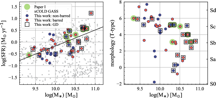
The left panel of Figure 1 shows the SFR– relation for our sample overlaid on a sample of local galaxies from the xCOLD GASS survey (grey circles; Saintonge et al. 2017). The integrated SFR and are derived based on GALEX and WISE (Leroy et al., 2019, 2021b). The line in the figure represents the local star-forming main sequence derived by Leroy et al. (2019). There are roughly equal numbers of galaxies above and below the main sequence. The offset from the main sequence (MS) spans 0.8 dex ( a factor of 6). Galaxies already included in the sample of Paper I are highlighted by a green circle (NGC 0628, NGC 3351, NGC 3627, NGC 4254, NGC 4321, NGC 4535, and NGC 5068).
We further classify our galaxies based on the presence of bar and grand-design spiral arms. In Figure 1, blue and red circles denote non-barred and barred galaxies, respectively, while the galaxies with grand-design spiral arms are marked by open squares. Information on the galactic structures is provided in Table LABEL:tab_galaxy_sampe_props. We define a galaxy as barred if a bar component was implemented in the PHANGS environmental masks (Querejeta et al., 2021) (morphbarflag in the PHANGS sample table version 1.5). These bar identifications mostly follow Herrera-Endoqui et al. (2015) and Menéndez-Delmestre et al. (2007), with some modifications based on the multi-wavelength and kinematic information available in PHANGS. For spiral arms, we adopt the flags morphspiralarms (i.e., grand-design spiral arms) from the PHANGS sample table, which comes from visual inspection of multi-wavelength data by four PHANGS collaboration members. Strictly speaking, the morphspiralarms flag in the sample table indicates whether the environmental masks include spiral masks or not. It is generally true that we implemented spiral arms mostly for grand-design spirals (and did not attempt to do so for flocculent arms). However, in some cases, e.g. due to inclination, we found that the spiral mask was not reliable even though the galaxy shows clear spiral arms and was classified as grand-design by Buta et al. (2015). Therefore, our classification does not always agree with arm classifications from the literature (e.g., Buta et al. 2015 for S4G222S4G: Spitzer Survey of Stellar Structure in Galaxies).
Morphology classification is presented by Hubble morphological T-type in this work. The T-type values for S0, and Sa – Sd galaxies are approximately -2, 1, 3, 5, and 7, respectively. Note that T-type considers ellipticity and strength of spiral arms, but does not reflect the presence or absence of the bar. The right panel of Figure 1 displays the Hubble type of our target galaxies as a function of . The Hubble type of the galaxies in our sample ranges from to 7.7 (approximately equivalent to S0–Sd). Our sample shows the expected trend: earlier types (i.e., smaller Hubble type values) are generally more massive (e.g., Kelvin et al., 2014; González Delgado et al., 2015; Laine et al., 2016), but the correlation is rather poor at the high-mass end of our sample of . In this work, we use the term “earlier” to denote galaxies with lower values of Hubble type, but note that our working sample does not contain elliptical galaxies; the earliest-type galaxy in our sample is NGC 4694 with Hubble type of 1.8 ( S0).
3 Methodology
This section introduces the method used to quantify the relative distribution of molecular gas traced by CO emission and recent star formation traced by H emission. The method is identical to that used in Paper I, with some changes in tuning parameter values.
3.1 H: Filtering Out Emission from Diffuse Ionized Gas
Our analysis uses H as a tracer for the location of recent high-mass star formation. However, H not only arises from H ii regions surrounding the massive stars that ionize them, but also the larger scale diffuse ionized gas (DIG). To correctly correlate the sites of star formation with molecular gas, our analysis must remove this diffuse component. DIG is warm ( 104 K) and low density ( 0.1 cm-3) gas found in the ISM of galaxies which seems similar to the warm ionized medium observed in the Milky Way (see the review by Haffner et al., 2009). The energy sources of DIG are still not well understood. Spectral features, such as the emission-line ratios and ionizing spectrum, of DIG are different from those of H ii regions powered by massive young stars (e.g., Hoopes & Walterbos, 2003; Blanc et al., 2009; Zhang et al., 2017; Tomičić et al., 2017, 2019), indicating the presence of additional sources of ionization. Since DIG constitutes a substantial fraction of the H flux in star-forming galaxies (e.g., Oey et al., 2007; Tomičić et al., 2021), one must remove the DIG contribution from the H fluxes when using H as a star-formation tracer.
Following the approach utilized in Paper I, a two-step unsharp masking technique is used to remove the DIG from the H images, We first identify diffuse emission on scales larger than H ii regions, and then we take into account higher levels of DIG contribution and clustering of H ii regions that are often found in galactic structures (e.g., spiral arms, Kreckel et al., 2016). More specifically, the following steps are undertaken to remove DIG in the original H images.
-
1.
Unsharp mask with a kernel of 200 pc. We smooth our original image with a Gaussian kernel with FWHM size of 200 pc, slightly larger than the largest H ii regions (Oey et al., 2003; Azimlu et al., 2011; Whitmore et al., 2011). Then we subtract this smoothed image from the original image. We identify initial H ii regions as the parts of the map still detected at high signal-to-noise in this filtered map. Specifically, first of all, peaks above 5 are identified, and then the mask is expanded to contain all connected regions that are above 3. H ii regions are identified as pixels enclosed within the masks.
-
2.
Subtract a scaled version of the initial H ii regions from the DIG map. We subtract a scaled version of the H ii regions identified in the previous step from the original map. The scaling factor is an arbitrary choice, but we do not want to over-subtract at this stage. A scaling factor of 0.1 is adopted in this work.
-
3.
Unsharp mask with a kernel of 400 pc. We smooth our H ii region-subtracted image with a Gaussian kernel that has FWHM of 400 pc, larger than that in Step 1. This scale is set such to detect higher levels of DIG contribution and clustering of H ii regions. Then, we subtract this smooth version of the image from the original image. We identify our final set of H ii regions in this filtered map using the same S/N criteria in Step 1.
On average, the DIG removal process removes 65% of the H emission across the sample, consistent with the DIG fractions of PHANGS galaxies measured by different approaches (Chevance et al., 2020; Belfiore et al., submitted). Moreover, our mean DIG fraction is in good agreement with the mean DIG fraction ( 60%) derived from H-surface brightness-based method for the 109 nearby star-forming galaxies in Oey et al. (2007). A similar mean DIG fraction is also suggested for CALIFA (The Calar Alto Legacy Integral Field Area Survey) galaxies based on integral-field-spectroscopy (IFS)-based H ii/DIG separator (Lacerda et al., 2018). The DIG fractions of our sample galaxies are provided in Table 2. We note that the tuning parameters adopted in this work are different from what was used in Paper I. The choice of parameters in this work is optimized to reproduce H ii regions identified with our PHANGS-MUSE IFS H-line images which have similar spatial resolution (Santoro et al., accepted). Changing the adopted kernel sizes has only a minor impact on the number of H ii regions but does affect their sizes. Therefore, a key assessment of the performance of the DIG removal strategy is to avoid H ii region overgrowth. This can be evaluated using emission-line ratios accessible via spectroscopic observations: for example, the [N ii]/H and [S ii]/H ratios are higher in the DIG relative to H ii regions (e.g., Hoopes et al., 1999; Blanc et al., 2009; Kreckel et al., 2016; Tomičić et al., 2017, 2021). The full catalog of H ii regions identified in our narrowband H maps, including a detailed description of how we verified the narrowband H ii regions using PHANGS-MUSE spectroscopic information and the dependence of DIG fraction on galaxy properties will be presented in a forthcoming paper (H.-A. Pan et al. in prep.). Our results remain qualitatively unchanged when using the tuning parameters in Paper I, as discussed in Appendix A.3. In this work, we assume all the H emission surviving from the DIG removal process is from H ii regions, and the contribution from other powering sources, such as AGN, post-AGB stars, and shocks, are statistically minor in the analysis. Separating these sources from H ii regions rely on emission-line diagnostics and therefore spectroscopic observations.
Here we note two important caveats of our DIG removal process. We use a signal-to-noise threshold when identifying H ii regions during the unsharp masking step. Since the noise and native resolution of the input H images vary, the effective H surface brightness threshold applied to our fiducial maps therefore also varies, corresponding to SFR surface densities of 10-3 – 10-2 M☉ yr-1 kpc-2 depending on the galaxy target333We adopt Equation (6) in Calzetti et al. (2007) for the relation between SFR and H emission, which assumes a Kroupa initial mass function.. For a point source at the native resolution of our H data, the effective sensitivity limits in terms of H surface brightness threshold applied to the fiducial maps corresponds to H ii region luminosities ()) between and , with most (80%) being between 37 and 38. The for our galaxies are listed in Table 3. The H ii region sensitivity limits are comparable to the turn-over point of the H ii region luminosity function measured by narrowband H imaging in the literature (e.g., Bradley et al., 2006; Oey et al., 2007), but we may miss the low-luminosity H ii regions detected by optical integral field units (Kreckel et al., 2016; Rousseau-Nepton et al., 2018; Santoro et al., accepted), which are unavailable at the necessary resolution for the bulk of the galaxies in our sample. Therefore, we may underestimate the number of sight lines with H emission (see Appendix A.4 for a detailed discussion on the impact of H sensitivity). Moreover, our H-line images are not corrected for dust attenuation, thus the maps may miss the most heavily embedded regions. Since our main analysis focuses mostly on the location (rather than the amount) of massive star formation, we consider internal extinction as a secondary issue. However, for some analysis based on flux, we may underestimate H flux for the regions where CO (and therefore dust) is present.
| galaxy | DIG | galaxy | DIG | galaxy | DIG |
|---|---|---|---|---|---|
| [%] | [%] | [%] | |||
| IC1954 | 70 | NGC2997 | 46 | NGC4569 | 62 |
| IC5273 | 73 | NGC3351 | 62 | NGC4571 | 68 |
| NGC0628 | 51 | NGC3511 | 65 | NGC4689 | 77 |
| NGC1087 | 49 | NGC3596 | 52 | NGC4694 | 91 |
| NGC1300 | 66 | NGC3626 | 86 | NGC4731 | 65 |
| NGC1317 | 80 | NGC3627 | 64 | NGC4781 | 74 |
| NGC1365 | 60 | NGC4207 | 74 | NGC4941 | 84 |
| NGC1385 | 49 | NGC4254 | 50 | NGC4951 | 80 |
| NGC1433 | 69 | NGC4293 | 88 | NGC5042 | 92 |
| NGC1511 | 64 | NGC4298 | 58 | NGC5068 | 52 |
| NGC1512 | 65 | NGC4321 | 58 | NGC5134 | 88 |
| NGC1546 | 79 | NGC4424 | 87 | NGC5530 | 66 |
| NGC1559 | 62 | NGC4457 | 81 | NGC5643 | 71 |
| NGC1566 | 48 | NGC4496A | 55 | NGC6300 | 58 |
| NGC2090 | 74 | NGC4535 | 78 | NGC7456 | 87 |
| NGC2283 | 57 | NGC4540 | 69 | ||
| NGC2835 | 41 | NGC4548 | 87 |
| galaxy | H res. | CO res. | 1 | galaxy | H res. | CO res. | 1 | ||
|---|---|---|---|---|---|---|---|---|---|
| [pc] | [pc] | [log(erg s-1)] | [M☉ pc-2] | [pc] | [pc] | [log(erg s-1)] | [M☉ pc-2] | ||
| IC1954 | 88 | 91 | 37.6 | 0.9 | NGC4293 | 53 | 88 | 36.7 | 1.5 |
| IC5273 | 77 | 120 | 37.4 | 0.8 | NGC4298 | 71 | 105 | 37.3 | 1.0 |
| NGC0628 | 41 | 53 | 37.0 | 1.5 | NGC4321 | 47 | 121 | 37.0 | 2.1 |
| NGC1087 | 69 | 123 | 36.9 | 1.8 | NGC4424 | 81 | 89 | 37.7 | 1.7 |
| NGC1300 | 73 | 95 | 36.8 | 3.1 | NGC4457 | 91 | 80 | 37.8 | 2.2 |
| NGC1317 | 74 | 147 | 37.3 | 1.6 | NGC4496A | 73 | 90 | 37.2 | 1.3 |
| NGC1365 | 58 | 130 | 36.9 | 2.4 | NGC4535 | 87 | 119 | 37.6 | 1.6 |
| NGC1385 | 85 | 105 | 36.9 | 2.6 | NGC4540 | 77 | 104 | 37.3 | 2.8 |
| NGC1433 | 74 | 62 | 37.1 | 1.6 | NGC4548 | 73 | 132 | 37.1 | 1.0 |
| NGC1511 | 84 | 107 | 37.8 | 0.9 | NGC4569 | 89 | 128 | 37.3 | 0.7 |
| NGC1512 | 67 | 90 | 36.8 | 1.4 | NGC4571 | 85 | 79 | 37.3 | 1.8 |
| NGC1546 | 125 | 114 | 37.6 | 0.7 | NGC4689 | 97 | 85 | 37.4 | 1.9 |
| NGC1559 | 129 | 117 | 37.7 | 1.5 | NGC4694 | 73 | 88 | 37.9 | 1.3 |
| NGC1566 | 62 | 104 | 36.9 | 2.0 | NGC4731 | 61 | 98 | 37.2 | 0.5 |
| NGC2090 | 52 | 73 | 36.9 | 1.0 | NGC4781 | 52 | 72 | 37.5 | 0.9 |
| NGC2283 | 54 | 87 | 37.5 | 1.5 | NGC4941 | 94 | 115 | 37.4 | 0.7 |
| NGC2835 | 56 | 50 | 37.2 | 1.7 | NGC4951 | 83 | 91 | 37.6 | 0.8 |
| NGC2997 | 64 | 92 | 36.8 | 1.3 | NGC5042 | 84 | 107 | 37.7 | 1.0 |
| NGC3351 | 56 | 70 | 37.4 | 1.4 | NGC5068 | 32 | 24 | 37.4 | 2.0 |
| NGC3511 | 75 | 121 | 37.4 | 0.4 | NGC5134 | 91 | 118 | 37.8 | 1.7 |
| NGC3596 | 63 | 65 | 37.4 | 3.0 | NGC5530 | 65 | 66 | 37.5 | 1.2 |
| NGC3626 | 148 | 114 | 38.4 | 2.5 | NGC5643 | 73 | 75 | 37.6 | 1.6 |
| NGC3627 | 80 | 86 | 37.3 | 1.3 | NGC6300 | 60 | 60 | 37.2 | 1.7 |
| NGC4207 | 70 | 93 | 37.6 | 2.0 | NGC7456 | 84 | 127 | 37.4 | 0.4 |
| NGC4254 | 59 | 107 | 37.2 | 3.1 |
3.2 CO: Applying a Physical Threshold
The CO images are treated using a similar scheme. We clip the CO images at our best-matching resolution of 150 pc using a threshold of 10 M☉ pc-2 accounting for galaxy inclination. This corresponds to a 3 sensitivity of our CO map with the lowest sensitivity at this spatial scale (Table 3). The applied threshold value is lower than the threshold used in Paper I (i.e., 12.6 M☉ pc-2) due to the lower sensitivity of the PAWS M51 observations. To have a data sample with homogeneous observational properties, M51 is not included in this work. Our results remain qualitatively unchanged if different clipping values are adopted (see Appendix A.5).
3.3 Measuring Sight Line Fractions
First of all, the thresholded H maps are regridded to match the pixel grid of the CO maps since the FoV of our ALMA observations is considerably smaller than that of narrowband observations. We convolve each thresholded CO and H image by a Gaussian to a succession of resolutions, ranging from our highest common resolution of 150 pc to 1500 pc, in steps of 100 pc. Then we clip the low-intensity emission in the convolved images. For each convolved image, we blank the faintest sight lines that collectively contribute 2% of the total flux in the image to suppress convolution artifacts. The results remain robust to small variations (1 – 4%) of this threshold.
Finally, we measure the presence or absence of the two tracers at each resolution in a FoV extending to 0.6 , which is the largest radial extent probed by our data in all galaxies, corresponding to 6.4 kpc on average (5 – 22 kpc, mostly 15 kpc). We divide each sight line (pixel) within 0.6 in the thresholded and artifact-clipped CO and H images into one of four categories:
-
•
CO-only: only CO emission is present
-
•
H-only: only H emission is present
-
•
overlap: both CO and H emission are present
-
•
empty: neither CO nor H emission is present444We note that the empty pixels in the filtered maps may contain DIG and/or CO emission with surface density below the applied threshold in the original maps..
The fraction of sight lines with (i.e., CO-onlyH-onlyoverlap) and without (i.e., empty) any emission are given in Table 4. At the highest common resolution of 150 pc, the median fraction of sight lines without any emission within 0.6 of our galaxies is as high as 70%, ranging from 13 – 97%. Moreover, the fractions of empty sight lines decrease with increasing spatial scales (Figure B.20, see also Pessa et al. 2021). The distributions of empty pixels among galaxies is a potentially interesting diagnostic of ISM evolution and host-galaxy properties. We defer a detailed analysis of the statistics relating to empty pixels to a future investigation, since the main focus of this paper is the impact of host galaxy properties and observing scale on the relative distribution of molecular and ionized gas.
We measure the fraction of sight lines and the fraction of flux in each region type, i.e., CO-only, H-only, and overlap, at each resolution. All galaxies in our sample have non-zero fractions for the three region types at the highest common resolution of 150 pc (Appendix B). Since we do not consider the sight lines where neither CO nor H emission is present, the sum of CO-only, H-only, and overlap sight lines is 100%. We also define CO sight lines as regions that are classified as either CO-only or overlap (i.e., sight lines with CO emission, regardless of whether they are associated with H emission or not), while H sight lines are defined as regions of H-only or overlap (i.e., sight lines with H emission, regardless of whether they are associated with CO emission).
| IC1954 | 48(52) | NGC1512 | 8(92) | NGC3596 | 46(54) | NGC4496A | 24(76) | NGC4941 | 20(80) |
|---|---|---|---|---|---|---|---|---|---|
| IC5273 | 33(67) | NGC1546 | 30(70) | NGC3626 | 7(93) | NGC4535 | 19(81) | NGC4951 | 30(70) |
| NGC0628 | 27(73) | NGC1559 | 50(50) | NGC3627 | 31(69) | NGC4540 | 40(60) | NGC5042 | 9(91) |
| NGC1087 | 58(42) | NGC1566 | 22(78) | NGC4207 | 40(60) | NGC4548 | 11(89) | NGC5068 | 31(69) |
| NGC1300 | 14(86) | NGC2090 | 40(60) | NGC4254 | 71(29) | NGC4569 | 15(85) | NGC5134 | 21(79) |
| NGC1317 | 12(88) | NGC2283 | 46(54) | NGC4293 | 3(97) | NGC4571 | 32(68) | NGC5530 | 42(58) |
| NGC1365 | 13(87) | NGC2835 | 29(71) | NGC4298 | 87(13) | NGC4689 | 45(55) | NGC5643 | 49(51) |
| NGC1385 | 39(61) | NGC2997 | 36(64) | NGC4321 | 41(59) | NGC4694 | 10(90) | NGC6300 | 48(52) |
| NGC1433 | 16(84) | NGC3351 | 22(78) | NGC4424 | 11(89) | NGC4731 | 10(90) | NGC7456 | 14(86) |
| NGC1511 | 37(63) | NGC3511 | 39(61) | NGC4457 | 26(74) | NGC4781 | 53(47) |
4 Results
4.1 CO and H Fractions at 150 pc Resolution
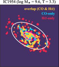
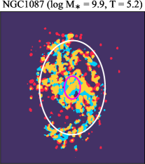
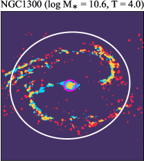
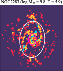
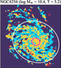
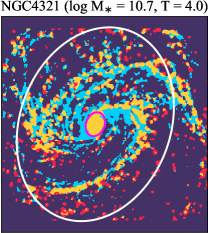
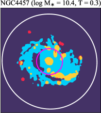
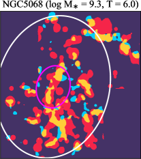
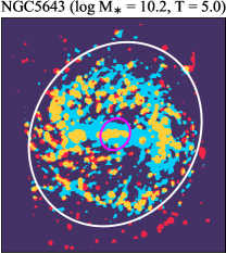
There are significant galaxy-to-galaxy variations in the CO and H distributions. Figure 2 presents some examples of the distribution of different sight line categories at 150 pc resolution (maps for the full sample are provided in Appendix B). The blue, red, and yellow regions denote CO-only, H-only, and overlap sight lines, respectively. We define the galactic center as the region within 1 kpc (i.e., 2 kpc in diameter) of the galaxy nucleus. The region that we define as the center is indicated in each panel as a magenta ellipse in Figure 2, while the region that we use to measure the global sight fraction is indicate as a white ellipse (i.e., 0.6 ).
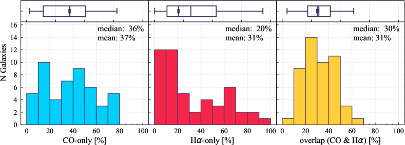
The histograms of Figure 3, from left to right, show the distribution of CO-only, H-only, and overlap fractions within the fiducial FoV at 150 pc scale, respectively. The boxplots shown at the top of each panel summarize the statistics for the sight line fractions. The sight line fractions for each individual galaxy are provided in Table LABEL:tab_fractions of Appendix B). The median and mean sight line fractions are given in the upper-right corner of the panels. In the rest of the paper, we will use the median as the measure of central tendency because the mean is more sensitive to extreme values. The mean values are given in the relevant figures and tables for reference.
We find a wide range of CO-only fraction in our sample from 3 to 78%, with a median of 36%. While the H-only fraction peaks at the lower end ( 20%), H-only sight lines show a wider range of spatial coverage than the CO-only sight lines, from nearly 0 to almost 95%. The median H-only fraction is 20%. The overlap region exhibits a narrower range than the CO-only or H-only regions, and shows a preference for intermediate values from 20 to 50%, with a median of 30%.
In terms of the relative frequency of the three types of sight lines, our results are qualitatively consistent with the conclusions of Paper I based on a smaller sample of only eight galaxies. However, Paper I reports considerably higher median values for CO-only and overlap sight lines (42% for CO-only and 37% for overlap) and slightly higher median for H-only (23%). We ascribe this difference to the combined effect of different thresholds for CO and H images and sample composition (e.g., distribution; see Figure 1 and next subsection).
4.1.1 Trends with Host Galaxy Properties
To explore the potential origin of the galaxy-to-galaxy variation in the spatial distributions of CO and H, we first compute the Spearman rank correlation coefficients between the sight line fractions and various host-galaxy and observational properties. The correlation coefficients are given in Table 5. In this work, a significant correlation is defined as a correlation coefficient of absolute value greater than 0.3.
The strongest correlations are found with and Hubble type for CO-only and H-only fractions. The fractions of CO-only and H-only regions are moderately correlated with , with correlation coefficients of 0.53 and , respectively. The CO-only and H-only fractions also correlate with Hubble type, with correlation coefficients of and 0.38, respectively. In contrast to the CO-only and H-only regions, overlap fractions show no significant correlation with and Hubble type in terms of correlation coefficients, 0.01 and 0.24, respectively.
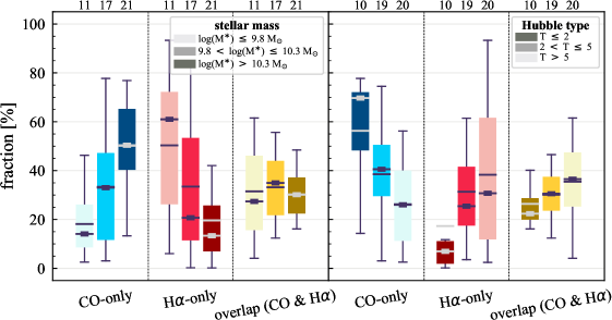
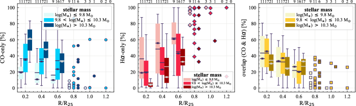
To further visualize the dependence of the sight line fractions on and Hubble type, Figure 4 shows boxplots of sight line fractions as a function of (left) and Hubble type (right). Galaxies are divided into three groups according to their or Hubble type. The darker colors indicate increasing or decreasing Hubble type value. The median and mean sight line fractions for a given or Hubble type are given in Table 6.
The left panel of Figure 4 shows a tendency for more massive galaxies to have higher CO-only fractions. The median CO-only fractions increase from 14% to 33% and to 50% from our lowest to highest bin. This dependency partially explains the higher median CO-only fractions in Paper I because that sample is largely dominated by galaxies with . An opposite trend is exhibited for H-only fractions, with the median fraction decreasing gradually from 61% to 21% and to 13%. Moreover, the two lower bins reveal a larger scatter in H-only fractions than for the highest bin, while the opposite trend is observed for CO-only sight lines. We note that the median H-only fraction in our highest- bin is lower than the median H-only fraction of galaxies with similar mass in Paper I because the H ii regions in this work are generally smaller than that in Paper I. This is driven by the different kernel sizes used in the unsharp masking technique to remove emission associated with the DIG. The median overlap fractions remain at a nearly constant value as a function of (27% to 35% and to 30%), but the scatter in overlap fraction decreases with increasing .
The trends with Hubble type and are consistent in the sense that late type galaxies tend to be less massive (right panel of Figure 4). The three Hubble type bins in the right panel of Figure 4 roughly correspond to earlier types than Sab (), around Sb–Sc (2 5), and later than Sc (). Unlike for , the overlap fraction shows an increasing trend toward the later-type galaxies. However, the differences in the overlap fraction between the different galaxy types are still significantly smaller than that for CO-only and H-only fractions, and the correlation coefficient (0.20) indicates a non-significant correlation.
We use partial rank correlation to examine whether the dependence of CO-only and H-only fractions on Hubble type is entirely due to the correlation with or the other way around. The partial rank correlation coefficient measures strength of the correlation between and when excluding the effect of . The partial rank correlation can be computed based on the Spearman rank correlation coefficient between the three variables as follows
| (2) |
where denoting the correlation between variables and . Using the rank correlation coefficients in Table 5 and Equation (2), the partial rank correlations between CO-only and H-only with become 0.35 and 0.32, respectively when Hubble type is controlled. The correlations between CO-only and H-only with Hubble type are 0.45 and 0.21 while holding . The partial correlation coefficients between these two sight line fractions with and Hubble type are lower than that of the bivariate coefficients. We therefore conclude that the correlations between CO-only and H-only fractions and both and Hubble type are physical in nature, but the correlation between and Hubble type may come between them. Such dependencies of sight line fractions (CO-only and H-only) on and Hubble type have also been hinted at by the small (8) galaxies sample in Paper I.
We also compute the correlation coefficients for the sight line fractions with other host-galaxy and observational properties: galaxy distance, optical size (), disk inclination, native resolution and effective sensitivity of the H ( in Section 3.1) and CO (1 at 150 pc resolution) observations, specific SFR (sSFR SFR/), and offset from the star-forming main-sequence (MS) (Table 5). Scatter plots of the sight line fractions as a function of all the properties we explore in this section are shown in Appendix C. Galaxies with lower are generally more nearby in our sample, caused by a potential sample-selection bias. Therefore, the dependence of sight line fractions on distance, sensitivity, and resolution might be a result of this selection effect. In principle, sight line fractions could correlate with DIG fraction, in the sense that removing a higher fraction of H flux would lead to a higher CO-only fraction and lower H-only and overlap sight lines. Such a dependence is seen in terms of correlation coefficients, but only for CO-only (0.31) and overlap regions (0.37). The sight line fractions show no significant correlation with other galaxy and observational properties we explore.
The CO-only fraction shows a correlation with sSFR (-0.32). At the same time, sSFR is correlated with , in the sense that along the star-forming main sequence, galaxies with higher tend to have lower sSFR (Brinchmann et al., 2004; Salim et al., 2007). We checked the partial correlation of CO-only fraction and sSFR taking as the control variable. The correlation between CO-only fraction and sSFR no longer exists (0.17) when is controlled for, but the correlation between CO-only and still holds while controlling for the effect of sSFR (0.47). This suggests that the correlation with sSFR is an outcome of the dependence on . There is no correlation between the sight line types and MS, which we discuss further in Section 5.3.
| CO-only | H-only | overlap | |
| galaxy properties | |||
| 0.53 | 0.44 | 0.01 | |
| Hubble type | 0.59 | 0.38 | 0.24 |
| distance | 0.39 | 0.28 | 0.09 |
| 0.08 | 0.02 | 0.17 | |
| inclination | 0.09 | 0.15 | 0.16 |
| DIG fraction | 0.31 | 0.08 | 0.37 |
| observations | |||
| effective H sensitivity | 0.30 | 0.18 | 0.14 |
| H native resolution | 0.38 | 0.25 | 0.13 |
| effective CO sensitivity | 0.25 | 0.39 | 0.36 |
| CO native resolution | 0.29 | 0.25 | 0.02 |
| star formation | |||
| sSFR | 0.32 | 0.17 | 0.20 |
| MS | 0.15 | 0.02 | 0.21 |
| log(/M☉) 9.8 | 9.8 log(/M☉) 10.3 | log(/M☉) 10.3 | |
|---|---|---|---|
| CO-only [%] | 14 (18) | 33 (33) | 50 (50) |
| H-only [%] | 61 (50) | 21 (33) | 13 (20) |
| overlap [%] | 27 (32) | 35 (33) | 30 (30) |
| T 2 | 2 T 5 | T 5 | |
| CO-only [%] | 70 (56) | 41 (39) | 26 (26) |
| H-only [%] | 7 (17) | 25 (31) | 31 (38) |
| overlap [%] | 22 (26) | 31 (30) | 36 (35) |
| log(/M☉) | 10.4 (10.3) | 10.4 (10.4) | 9.8 (9.9) |
4.1.2 Radial Distribution of CO and H Sight Lines
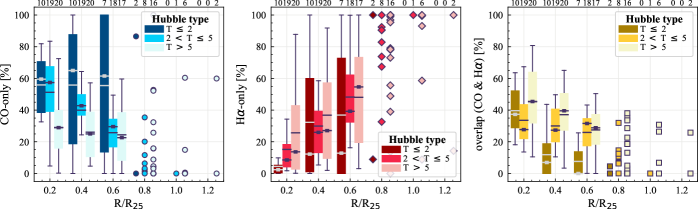
We quantify the radial trends of CO-only, H-only, and overlap fractions (from left to right) in Figure 5. Here, boxplots showing the galaxy distributions for each of the sight line fractions are shown as a function of deprojected galactocentric radius normalized to in annuli of width 0.2 . For each galaxy, we only compute its radial sight line fractions out to the maximum radius of complete azimuthal [0, 2] coverage. For each radial bin, the light to dark boxplots represent the distributions for the lowest (later) to highest (earlier) bins of (Hubble type). The three boxes at a given radius are offset by 0.05 on the plot for clarity. The number of galaxies in each radial bin is indicated above each panel. Some galaxies have maximum complete radius up to 1.2 . For reference, we show the sight line fractions of each individual galaxy at these radii using symbols rather than boxplots. Note that the data points at 0.6 regime are dominated by large spiral galaxies. Due to the biased sample and low number statistics, data at 0.6 are not included in our discussion. The color coding of each symbol is the same as for the boxplots at 0.6 .
The sight line fractions show a strong radial dependence. CO-only sight lines decrease with increasing radius and the fractions of H-only sight lines increase with radius. The ordering between sight line fractions and is observed in each radial bin at , suggesting that the dependence (or lack of dependence) of the total sight line fractions on and Hubble type in Figure 4 is driven by the local trends at all radii. The median CO-only fractions at is at least doubled when moving from the lowest to the highest bins. The radial profiles of H-only sight lines also show a clear ranking with at , increasing from the highest to the lowest bins. The differences between bins are considerably smaller for overlap regions, but it can be seen that the radial profile of overlap sight lines is shallower for the highest bin than the two lower bins. This is at least partially due to the fact that lower mass galaxies generally have lower CO-only fraction at larger radii than high mass galaxies; given that the overlap regions appear to be embedded in the CO-only regions (Figure 2), the chance to have overlap sight lines at large radii of lower mass galaxies is small.
The observed correlation between the sight line fractions and Hubble type in Figure 4 is also seen in most of the radial bins, but the rankings are not as obvious as for , partially due to lower number statistics for the earliest bin.
4.2 Trends with Galactic Structure
Molecular gas is preferentially formed or collected efficiently in galactic structures such as bars and spiral arms. Since the distribution of molecular gas subsequently determines the potential sites of star formation, it is natural to expect that the distributions of CO and H emission are also regulated by galactic structures.
We classify our target galaxies into four groups according to the presence and absence of bar and grand-design (GD) spiral arms:
-
1.
no structures (NS): galaxies without bar and GD spiral arms (e.g., galaxies with flocculent/multiple arms are in this category)
-
2.
Bar: galaxies with a bar but no GD spiral arms
-
3.
Bar+GD: galaxies with a bar and grand-design spiral arms
-
4.
GD: galaxies with grand-design spiral arms but without a bar.
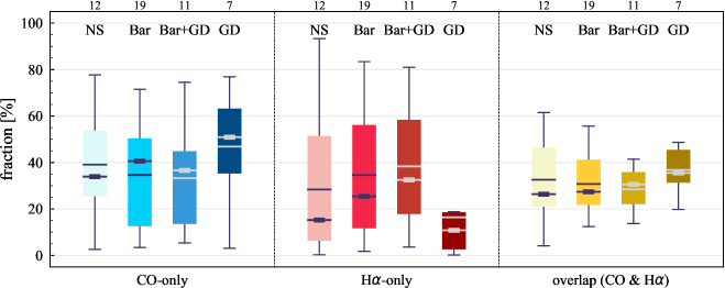
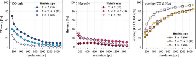
The number of galaxy in groups (1) to (4) are 12, 19, 11, and 7, respectively. The statistics of sight line fractions for each category at 150 pc resolution are provided in Table 7; the corresponding boxplots are shown in Figure 6. While the sight line fractions for NS, Bar, and Bar+GD span over a similar range, GD galaxies exhibits a distinct sign of higher CO-only and overlap fractions and lower H-only fractions than the other populations. Since GD galaxies have a lower median (log(/M☉) 10.3) than the Bar+GD galaxies (10.7) (Table 7), the differences in CO-only and H-only fractions between GD and Bar+GD are opposite to what one would expect if is the dominant driver of the sight line fractions, and points to the potential importance of galactic structure on regulating the star formation process.
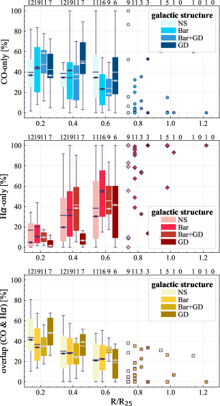
Figure 7 presents the radial sight line fractions for each structure type at 150 pc resolution. The bar length in our galaxy sample ranges from , with most bar lengths around . The median bar length of Bar+GD galaxies (0.3 ) is slightly longer than that of Bar galaxies (0.2 ). Galaxies with a bar (Bar and Bar+GD) visually show stronger radial dependence of CO-only sight lines than galaxies without a bar (NS and GD), in the sense that their median CO-only fraction gradually decreases with increasing radius. The opposite trend is observed for overlap regions. Moreover, Figure 7 suggests that the high total CO-only fraction in GD galaxies (Figure 6) is due to the increased fraction at . On the other hand, the low total H-only fraction can be attributed to a lack of H-only regions at .
In summary, the results in this section show that, in addition to global galaxy properties, galactic dynamics add a further layer of complexity to the distribution of CO and H emission. We note that the FoV covering fraction of galactic structures could affect the sight line fractions. For example, while bars are fully covered by our FoV, we may miss the outer part of some GD spiral arms. This analysis could be taken further by counting the sight lines within individual fully-sampled structures, but that is beyond the scope of this paper. We refer the reader to Querejeta et al. (2021) for a comprehensive empirical characterisation of the molecular gas and star formation properties in different galactic environments of PHANGS galaxies.
| no structure (NS) | bar only (Bar) | bar and GD spiral arms (Bar+GD) | GD spiral arms only (GD) | |
|---|---|---|---|---|
| CO-only | 34 (39) | 41 (35) | 37 (33) | 51 (47) |
| H-only | 15 (28) | 25 (35) | 32 (38) | 11 (16) |
| overlap | 26 (33) | 27 (31) | 31 (28) | 36 (37) |
| log(/M☉) | 9.9 (9.9) | 10.0 (10.0) | 10.7 (10.5) | 10.3 (10.2) |
4.3 CO and H Flux in Single-Tracer and Overlap Regions
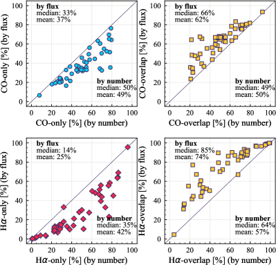
In this section, we explore whether there is any difference between regions where both tracers are observed (overlap) and regions where only one tracer is observed (CO-only and H-only). We estimate the fractional contribution of CO-only (i.e., only one tracer is observed) and overlap (two tracers are observed; CO-overlap) to the total CO sight lines, and the fractional contribution of H-only and overlap (H-overlap) to the total H sight lines. In other words, the sum of CO-only and CO-overlap is normalized to 100%, and so is the sum of H-only and H-overlap. To compare with the results based on the number of sight lines (our default fraction), the corresponding fractions for flux are also estimated.
Figure 8 shows the comparison of sight line fractions with flux fractions. Specifically, for each data point, the values on the - and -axis are calculated based on exactly the same pixels (sight lines), but the -axis shows their fractional contribution to the total sight line of the tracer and the -axis shows their fractional contribution to the total flux of the tracer. The black line indicates a one-to-one correlation.
The median sight line fractions of CO-only and CO-overlap are approximately equal (-axes in the upper panels of Figure 8), but the latter contributes a larger portion to the overall flux (66%; -axis of upper-right panel). Nonetheless, CO-only regions still contribute one third of the CO flux (33%; -axis of upper-left panel). The difference between the fractions by number of sight lines and by flux is larger for H, as shown in Figure 8 (lower panels). Taking all the pixels in our galaxies, the H-only accounts for 36% of the area of H-emitting regions, but contributes only 14% of the H flux. On the other hand, H-overlap contributes 85% to the total H flux, and it is higher than the 64% sight line fraction. Since the H-overlap regions are by definition co-spatial with CO-emitting molecular gas, they likely suffer from dust attenuation that we do not account for in the processing of our H maps due to the lack of extinction tracers (Section 2.2). Therefore, the true flux contribution of H-overlap is probably higher.
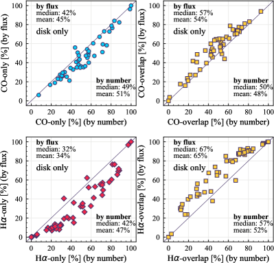
While covering only a small area, galaxy centers often substantially contribute to the total flux (Querejeta et al., 2021). Since the flux in the central region of galaxies is not necessarily associated with star formation, we therefore repeat the analysis while excluding the central 2 kpc in deprojected diameter (Figure 8). For CO, the agreement between area and flux is much tighter; the deviation from the one-to-one line for high CO fractions almost vanishes, implying that galactic centers drive the difference. On the other hand, H fractions appear less dominated by the centers. This is at least partially due to higher extinction present in the centers. The trend of higher flux in H-overlap regions than in H-only regions persists even when excluding the centers.
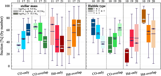
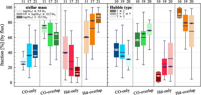
Figure 9 compares the fractions by number of sight lines (upper panel) and flux (lower panel) for galaxies in different and Hubble type bins. The distributions of CO-only and CO-overlap are shown by blue and green boxes, respectively, while H-only and H-overlap are shown by red and orange boxes. For each or Hubble type bin (indicated by the darkness of the boxes), the sum of a data point in the blue (red) box and the corresponding data point in the green (orange) box is normalized to 100. The median and mean for each and Hubble type bin are summarized in Table 8. The trends with and Hubble type are the same for sight lines and flux, but the difference among the and Hubble type bins are sightly larger when considering flux instead of number of sight lines. For all and Hubble type bins, the overlap regions contribute to a larger proportion of CO and H flux than regions with only one type of emission.
Interestingly, CO-only becomes dominant in the highest galaxies, occupying 60% of the CO-emitting regions. However, they are almost as equivalently low in flux contribution as other populations, implying a generally (i.e., more extended distributed) low H2 surface density in the highest galaxies in our sample. The same feature is seen for the earliest type galaxies, hinting that star-formation ceases to prevail over a significant area of a galaxy while gas remains there. However, we cannot rule out that this result arises from our methodology. Some CO-onlygas in the low-mass galaxies may not pass our threshold due to its intrinsically low , while in higher mass galaxies, their CO-onlygas is slightly brighter than our threshold. This would potentially add many CO-emitting sight lines, but very little flux. Such a possibility again highlights the differences in molecular gas properties among galaxies with different and Hubble type.
In summary, at 150 pc spatial scale, the fluxes of CO and H emission are higher in overlap regions where emission from both tracers is observed compared to regions where only one tracer is observed, consistent with the finding of Paper I. This trend holds for galaxies with different and Hubble type. Nonetheless, the contribution from regions with only one tracer (CO-only and H-only) to the total flux remain substantial for most systems.
| log(/M☉) 9.8 | 9.8 log(/M☉) 10.3 | log(/M☉) 10.3 | |
|---|---|---|---|
| sight line % median (mean) flux % median (mean) | |||
| CO-only | 34 (35) 24 (28) | 45 (46) 36 (36) | 57 (61) 36 (43) |
| CO-overlap | 66 (65) 76 (72) | 55 (54) 64 (64) | 43 (39) 64 (57) |
| H-only | 69 (58) 39 (41) | 32 (44) 18 (28) | 29 (34) 11 (15) |
| H-overlap | 31 (42) 61 (59) | 68 (56) 82 (72) | 71 (66) 89 (85) |
| T 2 | 2 T 5 | T 5 | |
| sight line % median (mean) flux % median (mean) | |||
| CO-only | 72 (65) 43 (45) | 55 (52) 35 (40) | 37 (40) 31 (31) |
| CO-overlap | 28 (35) 57 (55) | 45 (48) 65 (60) | 63 (60 69 (69) |
| H-only | 22 (27) 09 (13) | 42 (47) 21 (25) | 38 (46) 21 (32) |
| H-overlap | 78 (73) 91 (87) | 58 (53) 79 (75) | 62 (54) 79 (68) |
4.4 Distributions of CO and H as a Function of Spatial Scale
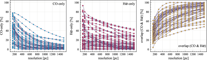
We investigate the impact of spatial scale on the distributions of CO and H emission. Figure 10 shows the sight line fractions for individual galaxies as a function of spatial scale from 150 pc to 1.5 kpc. For most of the galaxies, their CO-only sight lines decrease to 20% at spatial scale 800 pc, regardless of their CO-only fractions at spatial scale of 150 pc. The overlap regions substantially increase and become the dominant sight lines when resolution is degraded. This is the case for all galaxies in our sample, and the vertical ordering of overlap fractions among the galaxies is almost maintained until 1.5 kpc resolution. At the lowest resolution we consider, more than half of the regions are populated by both CO and H emission in most galaxies. While the variations of CO-only and overlap sight line fractions with spatial scale are rather uniform across the sample, the relation between H-only fractions and spatial scale is more diverse. Specifically, galaxies with low H-only fractions at 150 pc scale exhibit a low, roughly constant fraction toward large spatial scale (lower resolution); galaxies with the highest H-only fractional percentages at the best 150 pc scale decrease rapidly toward low resolutions; and some galaxies show increasing H-only fractions with decreasing resolutions. For all sight line categories, the variations with spatial scale become less evident at 500 pc resolution. The flattening point determines the critical resolution at which we stop resolving the CO and H distributions.
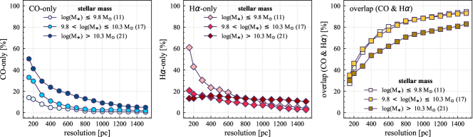
Figures 11 sheds light on the nature of the different H-only versus spatial scale relation. These figures are analogous to Figure 10, except that now galaxies are binned by their and Hubble type. The high global H-only fractions at 150 pc scale, which tend to be relatively isolated toward the outer parts of low- and/or later-type galaxies, become quickly contaminated by other types of sight lines in the inner regions when the resolution is lowered. In other words, we see that the CO-only and overlap regions increase in size and expand toward outer disks when the resolution decreases, e.g., NGC 2090, NGC 2835, and NGC 4951 in Figure B.20), leading to a rapid decrease of the H-only fraction as a function of increasing spatial scale. On the other hand, the H-only fraction of galaxies with low-H-only are less sensitive to resolution. They tend to be higher- galaxies. Their H-only sight lines populate both outer and/or inner disks (e.g., inter-arm regions, NGC 1300 and NGC 4321 in Figure 2 and NGC 2997 and NGC 3627 in Figure B.20). Whether a galaxy’s H-only fractions increases or decreases with resolution depends on the relative distribution of gas traced by CO and H.
By contrast, CO-only sight lines vary relatively uniformly as a function of spatial scale among different galaxy populations. The profiles show a clear ranking with and Hubble type at spatial scale 500 pc. At spatial scale 500 pc, the dependence of CO-only fraction on and Hubble type becomes less pronounced. While we find no strong dependence of overlap regions with at resolution of 150 pc (Figure 4), Figure 11 shows that galaxies in the highest bin tend to have lower overlap fractions when the spatial scales are larger than 300 pc. On the other hand, the trend with Hubble type at 150 pc resolution only holds when the spatial scale is smaller than 500 pc.
In summary, the results of this section demonstrate the important role that spatial scale can play when characterizing the distribution of CO and H emission and their dependence on host galaxy properties. The trend between sight line fractions and spatial scale was also observed in Paper I for individual galaxies, here we further show that the resolution dependence depends on galaxy type and the underlying high resolution CO and H emission structure, indicating that there may be no simple (universal) prescription to infer the physical connection between gas and star formation from kpc-scale measurements.
5 Discussion
We have analyzed a sample of 49 resolution-matched CO and H maps, which trace molecular gas and high-mass star formation, respectively. At the best resolution we consider, 150 pc, we find that the distributions of both CO and H emission depend on galaxy stellar mass and Hubble type (Section 4.1). Specifically, the CO-only fractions increase with stellar mass and earlier Hubble type, while the converse is seen for H-only fractions. The fraction of overlap regions remains roughly constant with both quantities.
Galactic structures act as an additional factor controlling the distribution of the CO and H emission (Section 4.2). GD galaxies exhibits a distinct sign of higher CO-only and overlap fractions and lower H-only fractions than the other populations; galaxies with a bar (Bar and Bar+GD) visually show stronger radial dependence of CO-only sight lines than galaxies without a bar (NS and GD).
However, probing the dependence of CO and H distributions on galaxy properties requires observations with resolution high enough to distinguish between regions where only one tracer is observed and regions where both tracers are observed (Section 4.4). Our results also show that, at 150 pc resolution, both CO and H tend to have higher flux in regions where both CO and H are found (overlap), than in regions where only a single tracer (CO-only and H-only) can be found (Section 4.3).
5.1 CO-only Sight Lines
We find that galaxies in our sample contain a substantial reservoir of CO-only molecular gas not associated with optical tracers of high-mass star formation (or above SFR surface densities of 10-3 – 10-2 M☉ yr-1 kpc-2 depending on the galaxy target). Our result is qualitatively consistent with studies of Local Group galaxies. In these galaxies (the Small and Large Magellanic Clouds (SMC and LMC) and M33), about 20–50% of GMCs are not associated with H ii regions or young clusters555Note that one should not compare the fraction of non-star-forming “GMCs” in the Local Group galaxies with our “sight line” fractions directly due to the different counting methods, i.e., object-based or pixel-based approaches. Direct comparison is only possible if we assume that GMCs have a fixed size, which is unlikely to be true (e.g., Hughes et al., 2013; Colombo et al., 2014; Rosolowsky et al., 2021). (e.g., Mizuno et al., 2001; Engargiola et al., 2003; Kawamura et al., 2009; Gratier et al., 2012; Corbelli et al., 2017). Our results further reveal that these starless clouds are not restricted to lower mass spiral and irregular galaxies, as in the Local Group, but are observed across the whole range of the galaxy population.
Non-star-forming gas: The sensitivity of PHANGS-ALMA is able to detect GMCs with mass of 105 M⊙; moreover, the CO-only sight lines are found at all surface densities from the adopted threshold to a few thousands of M⊙ pc-2. Massive star formation is certainly expected to proceed in these relatively high-mass and high density regions. This implies that part of the CO-only gas consists of non-star-forming clouds; the gas is unable to form stars because of its intrinsic properties. For example, molecular gas in some CO-only regions might be a diffuse, dynamically hot component (Pety et al., 2013) that is not prone to star formation, or may be analogous to the gas in the centers of early-type (elliptical) galaxies that seems not to be forming stars (Crocker et al., 2011; Davis et al., 2014). Nonetheless, we note that although the non-star-forming gas does not currently participate in the local on-going star-formation cycle, it may participate in star formation at some point in the future, i.e. made possible by relocating to a different, favorable site in the galactic potential that prompts a change in its dynamical state and/or organization, for example.
Low-mass star formation: It is possible that high-mass star formation is suppressed in the CO-only regions, forming stars that are not massive enough to produce detectable H emission. Such molecular clouds have been found in the Large Magellanic Cloud (Indebetouw et al., 2008).
Embedded star formation: Massive stars may be formed in part of the CO-only gas, but their H emission is obscured by dust. However, the embedded phase is relatively short, lasting only for a few to several Myr (Kim et al., 2021), and therefore may not account for all CO-only regions.
Pre- and/or post-star formation: The CO-only gas might be in the process of collapsing or may be remnant molecular gas dispersed from previous star-forming sites by stellar feedback (e.g., photoionization, stellar winds, and supernova explosions).
Distinguishing these scenarios requires the analysis of multi-wavelength data, such as line widths and surface densities of molecular clouds, dense gas tracers, better tracers of obscured star formation (e.g. infrared emission), and extinction tracers, but such an analysis is beyond the scope of this paper. Future James Webb Space Telescope (JWST) observations will also provide crucial insight into the complex processes of star formation and the nature of our CO-only sight lines.
In Section 4.4, we saw that the observed sight line fractions depend on spatial scale. We repeated our analysis for a subsample of 17 galaxies for which our observations achieve a common 90 pc resolution to test whether the fraction of CO-only sight lines in galaxies is larger at even higher physical resolution. A CO threshold of 13 M☉ pc-2 is adopted, corresponding to the 3 of the lowest sensitivity of these galaxies at 90 pc resolution. The CO-only fractions in all galaxies show an increase by 14% (median) as the resolution improves from 150 to 90 pc, while the fraction of H-only and overlap regions for the 90 pc maps decreases by 4% and 8%. This suggests that there remains a non-negligible fraction of CO-only gas that is not well resolved at our fiducial scale of 150 pc. If we increased the resolution even more, e.g., to 10 pc, we might expect to find even more CO-only sight lines, but testing this will require higher resolution ALMA observations. At some point, such observations will highly resolve individual clouds or other star-forming structures, and we might even detect that individual regions within a molecular cloud remain quiescent (e.g., genuinely non-star-forming or pre-star-forming) while stars already form elsewhere. This is not yet the case for our data, however.
5.2 Effect of Galactic Dynamics
Both bar and grand-design spiral arms are known to stabilize the gas against collapse and thus star formation under certain circumstances (Reynaud & Downes, 1998; Zurita et al., 2004; Verley et al., 2007; Meidt et al., 2013). However, while we indeed observe a higher fraction of CO-only sight lines in grand-design spiral galaxies (Figure 6), the CO-only fractions of Bar and Bar+GD are comparable to NS galaxies. It is probably because we do not consider bar strength in this work which is known to be correlated with SFR and star formation history of galaxies (Martinet & Friedli, 1997; Carles et al., 2016; Kim et al., 2017). An alternative explanation could be that the gas distribution in barred galaxies is evolving heavily over time (e.g., Donohoe-Keyes et al., 2019), leading to a wide variety in the gas distribution in the barred galaxies seen in PHANGS (Leroy et al., 2021b).
Nonetheless, our results show a possible trend for galaxies with bars (Bar and Bar+GD) to exhibit a stronger radial dependence in the fraction of CO-only sight lines (Figure 7). This may be attributed to bar-driven gas inflows which increase the gas concentrations in the central regions (Sakamoto et al., 1999; Sheth et al., 2005; Sun et al., 2020b). Moreover, the Bar and Bar+GD galaxies show a weaker radial dependence of overlap fraction than the NS and GD galaxies in terms of median values. Star-forming complexes are often observed at bar ends. Although bar footprints are not necessarily forming stars, the star-forming bar ends may smooth the profiles of the overlap sight lines (James et al., 2009; Beuther et al., 2017; Díaz-García et al., 2020). Finally, we note that we did not control for other trends (e.g., ) when comparing sight line fractions between galaxies with different structures. A very large sample is required in order to distinguish the effects of global galaxy properties and galactic dynamics.
Some galaxies show a pronounced offset between the different sigh line types with a sequence of CO-only to overlap and to H-only when going from up- to downstream (assuming the spiral arms are trailing, e.g., NGC 4321 in Figure 2 and NGC 0628, NGC 1566, NGC 2997 in Figure B.20), consistent with expectations for a spiral density wave (see Figure 1 of Pour-Imani et al., 2016). These offsets are almost exclusively found in well-defined grand-design spiral arms and presumably lead in turn to the high (or even highest) CO-only fraction in the disk (0.4 and 0.6 ) of GD in Figure 7, suggesting that most of GD structures may indeed be density waves. This demonstrates the potential of the sight line method as a diagnostic of the relationship between ISM condition and galactic dynamics. Detailed analysis of individual galaxies would be necessary to confirm the (dynamical) nature of our grand-design spiral arms.
Besides, the offsets between molecular gas and star formation tracers also allow measurement of the angular rotation velocity of a spiral pattern and the timescale for star formation (e.g., Egusa et al., 2004, 2009; Louie et al., 2013). While such analyses have been restricted to small-sample studies in the past, PHANGS allows for a systematic exploration of the spatial offset between the gas spiral arms and star-forming regions. Some barred galaxies also exhibit such CO-only and overlap offsets along their spiral arms, e.g. NGC 4321 and NGC 3627 in Figure 2 and NGC 1365 in Figure B.20, suggesting a dynamical link between spiral arms and stellar bar (Meidt et al., 2009; Hilmi et al., 2020).
5.3 Sight Line Fractions and Star Formation
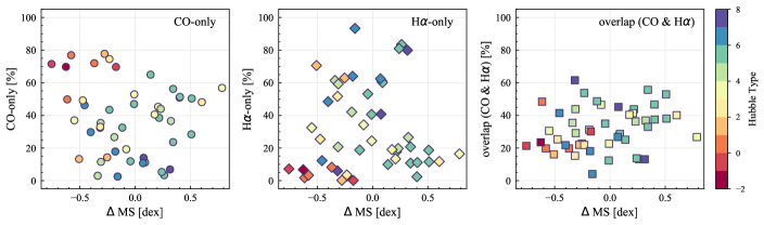
We find no correlation between sight line fractions and star formation properties (Section 4.1.1) and no correlation with the fractions of flux contributed by CO-only, H-only, CO-overlap, and H-overlap regions (correlation coefficients 0.2). Figure 12 shows the sight line fractions against MS, color-coded by Hubble type. Although there is no statistical relationship between the sight line fractions and MS, galaxies with low MS in our sample, dex or 4 times below the main sequence (NGC 1317, NGC 3626, NGC 4457, and NGC 4694), tend to have high CO-only sight line fractions ( 50–80%). These low-MS galaxies are all earlier types with Hubble type (S0–Sa). The spatial distribution of their CO-only regions are relatively compact inner disks, analogues to the molecular gas in elliptical galaxies (e.g., Crocker et al., 2011; Davis et al., 2014). By contrast, among the six highest-MS galaxies ( 0.4 dex or 2.5 times above the main sequence) in our sample, four show relatively high CO-only sight line fractions ( 50%; NGC 1365, NGC 1559, NGC 4254, and NGC 5643). All these high-CO-only and high-MS galaxies have grand-design spiral arms and/or a bar; moreover, their CO-only sight lines follow well these galactic structures, implying a dynamic origin of the high CO-only fractions. Although both galaxies with the highest- and lowest-MS in our sample show substantial CO-emitting regions not associated with star formation, the spatial distribution of their CO-only regions is markedly different, potentially pointing to different underlying causes for the suppressed star formation in these regions.
The other two highest-MS galaxies (NGC 1385 and NGC 1511) have lower, but not necessarily low, CO-only fractions (28 and 48%). Both of them happen to be peculiar systems. In fact, four out of the six highest-MS galaxies (NGC 1365, NGC 1385, NGC 1511, and NGC 4254) show signs of interactions with other galaxies.
In our working sample, 33 galaxies show signs of interactions in terms of their morphology. The median overlap sight line fraction of the merger candidates (28%) is slightly lower than that of isolated galaxies (36%). However, the overlap sight lines in the merger candidates contribute a higher fraction flux (90%) to the total H flux than for the apparently undisturbed galaxies (73%). Taking these numbers at face value, a given unit of star-forming region (overlap) in merger candidates contribute more significantly to the total SFR of a galaxy than a given unit of star-forming region in undisturbed galaxies, assuming that all the H emission is powered by star formation. We should note that galaxy interactions may trigger central AGN (e.g., Ellison et al., 2019) and shocks prevailing over the disks, which could contribute to H emission. However, we are not able to cleanly separate H ii regions from other H-emitting sources when using only narrowband data. Spectroscopic observations are necessary to confirm the differences between merger candidates and undisturbed galaxies.
5.4 H Sight Lines at Large Galactocentric Radii
The H-only sight lines are preferentially found at large galactocentric radii and even become dominant at 0.4 ( 60%) in low- galaxies. Moreover, the fraction of H-only sight lines is always higher for low- galaxies than higher- galaxies at all radii (Figure 5). The lack of CO sight lines at large radii may be due to (1) the lack of gas and/or (2) the existence of low- gas that drops below our applied threshold (Section 3.2).
To gain insight into the extent of cold gas reservoirs in our galaxies, we compute the radial profiles of gas fractions () and molecular-to-atomic gas mass ratio () for galaxies that have spatially-resolved measurements of atomic gas and stellar mass surface densities ( and ). is defined as the ratio of the total gas mass ( +) to , while is defined as the ratio between and . The spatially-resolved HI data are taken from various sources in the literature, including the PHANGS-VLA (D. Utomo et al. in prep.), VLA THINGS (Walter et al., 2008) and VIVA (Chung et al., 2009) surveys, and VLA archive. The spatially-resolved are measured based on Spitzer IRAC 3.6m or WISE 3.4m (Leroy et al., 2019, 2021b). The typical resolution of and measurements is 1 – 2 kpc. Since we are interested in the general trend of the and distributions, high spatial resolution is not needed for this purpose. In total, for 28 and 32 galaxies we can compute their radial and , respectively. For this analysis, we rely on radial measurements at matched kpc resolution from the PHANGS multi-wavelength database presented in Sun et al. (2020b) and J. Sun et al. (in prep.).
Figure 13 shows the radial (upper row) and (lower row) for galaxies with different (left) and Hubble type (right). Our sample shows a gradual decrease of with increasing at all radii. Moreover, increases with (when looking at 0.6 ). The trends with Hubble types are consistent in the sense that later type galaxies are less massive. The results in Figure 13 are in good agreement with Saintonge et al. (2011, 2016) based on integrated measurements for a large sample of galaxies
Furthermore, Figure 13 shows that the high-H-only regime () of low mass galaxies still harbors a significant reservoir of gas with respect to stellar mass ( 0.2), but the gas is predominantly atomic ( 1). Therefore, it is likely that there are molecular clouds in the outer atomic-dominated, high-H-only regions, but their is low and below our applied threshold.
For galaxies with log(/M⊙) 10.3, around 70–98% of the total CO emission (both median and mean are 90%) are included in our analysis of sight line fractions (i.e., 10 M☉ pc-2), while the fraction of CO emission above our applied threshold decreases to 40–90% (both median and mean are 65%) for log(/M⊙) 10.3. We also observe a stronger variation in the H-only fractions for low- galaxies when lowering CO threshold while keeping H threshold fixed. These imply a prevalence of lower mass molecular clouds ( M☉) in lower-mass galaxies and significant galaxy-to-galaxy variations in their molecular cloud properties (e.g., Hughes et al., 2013; Schruba et al., 2019; Sun et al., 2020a, b; Rosolowsky et al., 2021). The galaxy-to-galaxy variations in cloud properties also leads to the correlations, albeit relatively weak, between the sight line fractions and CO effective sensitivity in Table 5. Moreover, the gas depletion time of molecular gas () is found to anti-correlate with galaxy , with lower- galaxies showing shorter even after accounting for the metallicity dependence of (Utomo et al., 2018). The - relation also causes substantial H emission not associated with molecular gas in low- galaxies.
Finally, dissociation is presumably more efficient in low- environments due to less dust shielding (e.g., Wolfire et al., 2010). Therefore, CO emission is preferentially seen in high-extinction regions (e.g., inner galactic disks). The need for high extinction to form CO may lead to the consequence that the radial profiles of CO are steeper than that of H (e.g., Leroy et al., 2008). Since decreases rapidly with increasing galactocentric radii, the choice of threshold has a significant impact on the overlap fractions at large galactocentric radii, especially for low- galaxies, whose are systematically lower (e.g., Hughes et al., 2013; Sun et al., 2020b).
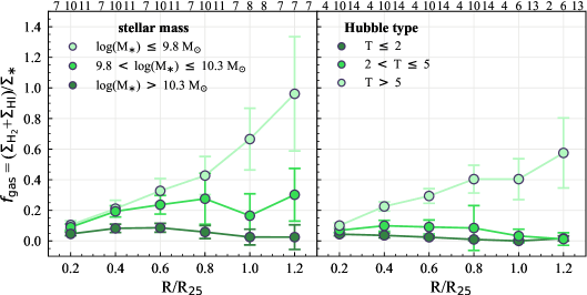
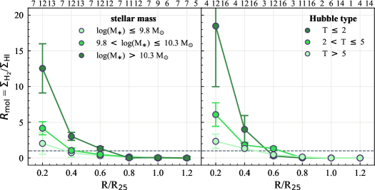
5.5 Relative Timescale of the Gas-Star Formation Cycle
If we assume that all the CO-only sight lines are pre-star-forming clouds, the three categories of regions we define roughly sample the evolutionary sequence of star-forming regions, in the sense that a cold molecular gas cloud (CO-only) evolves into a star-forming molecular cloud (overlap), and then to a region of (exposed) massive young stars (H-only) where the molecular gas has been largely dispersed and/or dissociated. In this scenario, the areal fractions that we measure are an approximate reflection of the time spent by a star-forming region in each of these different evolutionary phases. Similar frameworks (i.e., counting the number of GMCs and H ii regions) have been applied previously to estimate the duration for which the molecular cloud traced by CO emission is visible in the LMC (Kawamura et al., 2009), constrain the cloud life-cycle in M33 (Gratier et al., 2012; Corbelli et al., 2017), and determine the timescales for dense molecular clumps to evolve from being starless to star-forming in the Milky Way (Battersby et al., 2017).
The evolution of molecular clouds provides constraints on the mechanisms triggering or halting star formation at a specific location in a galaxy. In Paper I, we apply a simple version of the approach to estimate the duration that molecular gas traced by CO emission is visible ():
| (3) |
where represents the duration that H emission from H ii regions is visible. , , and denote the fraction of CO-only, H-only, and overlap sight lines, respectively. Then represents the scaling factor to translate from the fiducial timescale, here , to 666We note that the cloud visibility time is different from the dynamic timescale or the depletion time. A comparison of various relevant timescales, such as cloud visibility time, free fall time, crossing time, and the characteristic timescale for star formation regulated by galactic dynamical processes has been discussed in Chevance et al. (2020) for a subset of PHANGS galaxies. A further discussion will also be presented in the upcoming paper by J. Sun et al. (in prep.).. We emphasize that, by applying Equation (3), we are implicitly assuming that our individual pixels are discrete star-forming units and all the CO-only sight lines contain pre-star-forming clouds (see Section 5.1).
Figure 14 shows the radial trend in averaged in bins of (upper panel) and Hubble type (lower panel)777 has to be calculated in radial bins or in any region-by-region manner, otherwise is heavily determined by the bright CO in the inner part and bright H in the outer part, but those regions do not form part of the same evolutionary cycle.. There is a ranking of along where molecular clouds in high- galaxies tend to have longer than clouds in low- over the radial range probed. Given that typical estimates for are 5–10 Myr (e.g., Leroy et al., 2012; Kennicutt & Evans, 2012; Haydon et al., 2020), the of our sample at 150 pc scale, therefore, decreases from 5 –25 Myr for the high- galaxies, to 5 –15 Myr for the intermediate- galaxies, and to a few Myr for the low- galaxies in our sample when applying a CO threshold of 10 M☉ pc-2. also decreases from earlier- to later-type spiral galaxies, but the trend is not as strong as for .
The dependence of on host galaxy properties suggests the potential importance of environment for regulating star formation (see also Paper I and Chevance et al. 2020). However, the evolution of star-forming regions is only visible when the spatial scale is close enough to the typical region separation length between molecular clouds and H ii regions. Figure 15 shows the dependence of radial on spatial scale as a function of . Light to dark gray circles denote at different spatial scales of 300, 500, 1000, and 1500 pc, while at 150 pc resolution is indicated by red squares. At spatial scales 300 pc, there is a distinct difference in between galaxy populations, as parameterized by . The differences between galaxies become considerably smaller at spatial scale of 300 pc due to the significant decrease in CO-only sight lines and increase in overlap sight lines, indicating a critical resolution requirement to resolve the evolution of individual star-forming regions. The critical spatial scale of 300 pc is consistent with the characteristic separation length between independent clouds or star-forming regions reported by Chevance et al. (2020).
While there is a clear dependence on spatial scale, the derived at 150 pc resolution are in reasonable agreement within a factor of a few (two to three) in most radial bins with the cloud lifetime () during which CO emission is visible estimated by Chevance et al. (2020) for seven of our galaxies using the statistical method developed by Kruijssen et al. (2018). We present a direct comparison of the radial variation of our with from Chevance et al. (2020) in Appendix D. The measured at 150 pc resolution also agrees well with the estimates of cloud (CO) visibility time based on counting the number of GMCs with and without H ii regions (e.g., Kawamura et al., 2009).
Finally, there are several systematic differences in cloud properties and uncertainties to bear in mind when using Equation (3) to estimate the visibility time of molecular clouds traced by CO. First of all, more massive galaxies typically have larger mid-plane ISM pressures, which leads to higher molecular gas surface densities and thus larger GMC sizes traced by CO. On the other hand, in a high-pressure environment, H ii regions might be smaller. Therefore, the number of CO and H sight lines may reflect not only the variation of cloud visibility time, but also the intrinsic differences in GMC and H ii region properties among galaxies. Moreover, our measurements of H sight lines (Section 3.1) is affected by internal extinction and non-H ii powering mechanisms. In principle, the identification of H ii sight lines could be refined by the use of optical IFS observations. Similarly, the fractions of CO sight lines depend on the applied surface density threshold (Section 3.2). Though our filtering methods are verified by visual inspection of the filtered CO and H images and comparing with the H ii regions identified in the PHANGS-MUSE images, the impact of methodology remains a potential source of bias (see Appendix A). Finally, molecular clouds and H ii regions may have not yet been fully resolved by our 150 pc resolution as discussed in Section 5.1. A handful of our galaxies have PHANGS-ALMA CO and PHANGS-MUSE H images with a resolution of 50 pc, comparable to the size of GMCs and H ii regions (e.g., NGC 0628, NGC 2835, and NGC 5068). At such high resolution, counting number of objects and sight lines should become almost identical, and thus would provide a more robust estimate on cloud (CO) visibility time and even the actual lifetime of molecular clouds. In summary, in addition to cloud visibility time, the region sizes traced by CO and H emission, the ratio between the resolution and the region separation length, and the data processing strategy may also contribute to the derived .
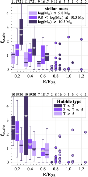
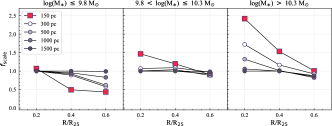
5.6 Implication for the Kennicutt–Schmidt Relation
Many studies have shown that the Kennicutt–Schmidt relation between the surface densities of molecular gas and SFR is tight with an index 0.7–1.4 on kpc scales (e.g., Bigiel et al., 2008; Leroy et al., 2008; Schruba et al., 2011; Leroy et al., 2013; Momose et al., 2013). These findings resonate with our analysis, where overlap sight lines dominate the maps when spatial scale is approximately or greater than 1 kpc; in other words, maps of molecular gas and star formation tracers become very similar.
The picture becomes more complex when the resolution increases. When the resolution is high enough to separate molecular clouds and star-forming regions, molecular gas and star formation surface densities become loosely correlated (e.g., Blanc et al., 2009; Onodera et al., 2010; Kreckel et al., 2018; Pessa et al., 2021) or even anti-correlated (e.g., Schruba et al., 2010) because the two components no longer coincide at all times. This spatial separation between different evolutionary stages of the star formation process is also evident in our sight line maps at the resolution of 150 pc (Figure 2 and Figure B.20). The loosely (anti-)correlated molecular gas and SFR tracers lead to an increasing scatter in the Kennicutt–Schmidt relation at small spatial scales, as a result of incomplete sampling of different evolutionary stages of the gas and star formation cycle (e.g., Schruba et al., 2010; Feldmann et al., 2011; Leroy et al., 2013; Kruijssen & Longmore, 2014).
Our results at 150 pc resolution reveal an important dependence between host galaxy properties and the relative distribution of molecular gas and star formation tracers to each other. Namely, how molecular gas and SFR tracers relate (or do not relate) to one another on the Kennicutt–Schmidt plane depends on the host galaxy properties, such as and Hubble type. However, any relation between the sight line fractions and host galaxy properties seen at 150 pc resolution is gradually diminished as resolution decreases, and becomes non-identifiable when at resolutions coarser than 500 pc. Galactic structures add a further complexity to the Kennicutt–Schmidt relation as the relation varies among galactic environments (Pan & Kuno, 2017; Pessa et al., 2021; Querejeta et al., 2021). Since the contribution of the different environments varies as a function of galactic radius, the impact of environments could be transferred to the Kennicutt–Schmidt relation when averaging the environments.
Moreover, if the relative distributions of CO-only and H-only sight lines are complex at high resolution, we might be missing important variations (i.e., slope and intercept of Kennicutt–Schmidt relation) and change in cloud life cycle/time variations (i.e., scatter of the relation) when using Kennicutt–Schmidt relation alone as a diagnostics of star formation process because the relation, by definition, only sees the overlap regions.
6 Summary
The main goal of this study is to investigate how global galaxy properties affect the radial distribution of various stages in the star formation cycle using an unprecedented large sample of 49 star-forming main sequence disk galaxies (Figure 1). We compare high resolution ( 1) observations of CO line emission and narrowband H maps of nearby galaxies selected from the PHANGS surveys (Section 2).
We adopt a simple and reproducible method developed in Paper I to quantify the relative spatial distributions of molecular gas and recent star formation (Section 3). The method has taken into account the contribution of diffuse ionized gas to the H emission and the metallicity dependence of CO-to-H2 conversion factor when identifying star-forming regions and molecular clouds.
We classify each sight line (i.e., pixel) at each resolution according to the overlap between the tracers: CO-only, H-only, and overlap (CO and H) (Figure 2). These three categories can be translated into the following star formation phases: CO-only – molecular gas currently not associated with star formation traced by H, overlap – star-forming molecular clouds, and H-only – regions of young massive stars. We investigate whether the fractions of the different categories of sight lines vary with galaxy properties (stellar mass and Hubble type), galactocentric radius, and the presence of bars or grand-design spiral structure. We also measure the sight line fractions at different resolutions ranging from 150 pc to 1.5 kpc. The best common resolution (150 pc) is sufficiently high to sample individual star-forming unit and to separate such regions. A summary of the main results presented in this paper is as follows.
-
1.
At our best-matching resolution of 150 pc for our sample, a median of 36% of detected sight lines in a galaxy are dominated by CO emission alone. The molecular gas surface densities of these CO-onlyregions are not necessarily low, ranging from our applied threshold (10 M☉ pc-2; see Section 3) to a few thousands M☉ pc-2. This implies that there is a substantial fraction of molecular gas in galaxies that is currently not associated with young high-mass star formation traced by non-DIG optical tracer. Statistically, the second most common category are overlap regions where both CO and H emission coincide, accounting for a median 30% of the sight lines at 150 pc resolution. The overlap sight lines show the least variation from galaxy to galaxy. The H-only sight lines are less common than the other two categories, with a median fraction of 20%, but also exhibit the largest galaxy-to-galaxy variations. The rank of the median sight line fractions is consistent with Paper I which used only eight galaxies (Section 4.1 and Figure 3).
-
2.
At 150 pc resolution, we find strong correlations between the sight line fractions (CO-only and H-only) and global galaxy properties. Such dependencies had already been hinted at by Paper I which analyzed a small subset of our sample; in this work, we quantify the dependencies. Specifically, the fraction of CO-only sight lines within the fiducial field of view increases gradually with increasing and also increases gradually from later to earlier type spiral galaxies. The opposite trend is observed for H-only sight lines. The fraction of overlap regions is insensitive to , but increase toward later types. These trends observed for global sight line fractions are almost preserved radially from the center out to 0.6 (corresponding to 6 kpc). Our results at 150 pc resolution suggest that the relationship between molecular gas and SFR tracers in the Kennicutt–Schmidt plane depends on host-galaxy properties (Sections 4.1 and 5.6, Figures 4 and 5).
-
3.
In addition to and Hubble type, we also classify galaxies according to the presence of a stellar bar and/or grand-design spiral arms. Galaxies without these structures, galaxies with a stellar bar only, and galaxies with both a bar and grand-design spiral arms exhibit broadly similar sightline fractions. Galaxies with grand-design spiral arms but no stellar bar, however, show a distinct signature of higher CO-only and overlap fractions and lower H-only fraction than the other populations. Moreover, galaxies with a bar show a stronger (weaker) radial dependence of CO-only (overlap) sight lines than galaxies without a bar. These results suggest that galactic dynamics further contributes to organizing the spatial distribution of CO and H emission separately within galaxies (Sections 4.2 and 5.2, Figures 6 and 7).
-
4.
Comparing the fractions of pixels (our “default” approach) with the fractions of flux shows that overlap regions tend to have higher CO and H intensities compared to regions that emit CO or H alone. Yet the flux traced by CO-only and H-only regions cannot be neglected, since they still contribute a median of 33% (mean: 37%) and 14% (mean: 25%) of the galaxy’s total CO and H flux, respectively. The result is consistent with the finding of Paper I. (Section 4.3, Figures 8 and 9).
-
5.
The sight line fractions show a strong dependence on spatial scale (resolution), confirming the finding of Paper I. Specifically, CO-only and H-only regions rapidly vanish as spatial scale increases. Therefore, any relation between the sight line fractions and galaxy properties ( and Hubble type) are only evident when the resolution is 500 pc (Section 4.4, Figures 10 and 11).
-
6.
We find no correlation between the global sight line fractions with specific star formation rate and the offset from the star-forming main sequence (MS). Nonetheless, galaxies with the highest- or the lowest-MS in our sample both show significant molecular gas reservoirs that appear not to be associated with star formation. However, the spatial distribution of their CO-only sight lines are different, pointing to different underlying causes of their high CO-only fractions (Section 5.3 and Figure 12).
-
7.
H-only regions tend to be found in atomic gas dominated regions in low- systems. It is very likely that lower mass molecular clouds exist in these regions, but their drops below our applied threshold, adding further evidence for prominent galaxy-to-galaxy variation in molecular cloud properties, in line with previous studies (e.g., Hughes et al., 2013; Sun et al., 2020b; Rosolowsky et al., 2021) (Section 5.4 and Figure 13).
-
8.
We estimate the the duration for which the molecular cloud traced by CO emission is visible following the statistical approach in Paper I. There is a ranking of cloud visibility time with where molecular clouds in high- galaxies tend to have a longer visibility time than clouds in low- over the radial range probed. The trend is related to the fact that molecular clouds in high- galaxies tend to have higher molecular mass surface densities. However, the differences between galaxies become considerably smaller when the spatial scale is larger than 500 pc due to a significant decrease in CO-only sight line and increase in overlap sight line, indicating a critical resolution that is required to resolve the evolution of individual star-forming regions. We also note several systematic differences in cloud properties and uncertainties to bear in mind when using Equation (3) to estimate the visibility time of molecular clouds (Section 5.5 and Figures 14 and 15).
The methodology presented in this paper offers a simple, physically motivated, and reproducible approach for quantifying the relative distribution of molecular gas traced by CO emission and HII regions traced by H emission. Several caveats related with the use of this approach should be kept in mind, including the choices of CO-to-H2 conversion factor, CO(2-1)-to-CO(1-0) brightness temperature ratio, unsharp masking parameters, and H and CO() thresholds. These factors are discussed in detail in Appendix A. Although our results remain robust when accounting for the impact of these factors, care should be taken when interpreting the results based on our sight line method. Moreover, since our main analysis focuses mostly on the location (rather than the amount) of massive star formation, we consider internal extinction as a secondary issue. Nonetheless, there is room for improvement with the use of optical IFS data which allows for simultaneous correction for internal extinction and tools for distinguishing H emission emitted from various powering sources. A straightforward next step would be to test our results with large, diverse, deep ( 36 erg s-1), and high resolution ( 100 pc) IFS sample. Other follow-up studies (utilizing a large IFS sample) include the detailed investigation of the nature of CO-only and H-only regions, the absolute timescale of each star formation phase, and the dependence of these properties on global galaxy properties and galactic dynamics.
We thank the anonymous referee for constructive comments that improved the paper. This work was carried out as part of the PHANGS collaboration.
HAP acknowledges funding from the European Research Council (ERC) under the European Union’s Horizon 2020 research and innovation programme (grant agreement No. 694343), and the Ministry of Science and Technology (MOST) of Taiwan under grant 110-2112-M-032-020-MY3.
ES, PL, DL, RMcE, TS, FS, and TGW acknowledge funding from the European Research Council (ERC) under the European Union’s Horizon 2020 research and innovation programme (grant agreement No. 694343).
AH was supported by the Programme National Cosmology et Galaxies (PNCG) of CNRS/INSU with INP and IN2P3, co-funded by CEA and CNES, and by the Programme National “Physique et Chimie du Milieu Interstellaire” (PCMI) of CNRS/INSU with INC/INP co-funded by CEA and CNES.
The work of AKL, JS, and DU is partially supported by the National Science Foundation under Grants No. 1615105, 1615109, and 1653300.
AB and FB acknowledge funding from the European Research Council (ERC) under the European Union’s Horizon 2020 research and innovation programme (grant agreement No.726384/Empire).
MC gratefully acknowledges funding from the Deutsche Forschungsgemeinschaft (DFG) through an Emmy Noether Research Group, grant number KR4801/1-1 and the DFG Sachbeihilfe, grant number KR4801/2-1, and from the European Research Council (ERC) under the European Union’s Horizon 2020 research and innovation programme via the ERC Starting Grant MUSTANG (grant agreement number 714907).
EC acknowledges support from ANID project Basal AFB-170002.
CE acknowledges funding from the Deutsche Forschungsgemeinschaft (DFG) Sachbeihilfe, grant number BI1546/3-1.
CMF is supported by the National Science Foundation under Award No. 1903946 and acknowledges funding from the European Research Council (ERC) under the European Union’s Horizon 2020 research and innovation programme (grant agreement No. 694343).
SCOG and RSK acknowledge financial support from the German Research Foundation (DFG) via the collaborative research center (SFB 881, Project-ID 138713538) “The Milky Way System” (subprojects A1, B1, B2, and B8). They also acknowledge funding from the Heidelberg Cluster of Excellence “STRUCTURES” in the framework of Germany’s Excellence Strategy (grant EXC-2181/1, Project-ID 390900948) and from the European Research Council via the ERC Synergy Grant “ECOGAL” (grant 855130).
JMDK gratefully acknowledges funding from the Deutsche Forschungsgemeinschaft (DFG) in the form of an Emmy Noether Research Group (grant number KR4801/1-1) and the DFG Sachbeihilfe (grant number KR4801/2-1), and from the European Research Council (ERC) under the European Union’s Horizon 2020 research and innovation programme via the ERC Starting Grant MUSTANG (grant agreement number 714907).
JP acknowledges support from the Programme National “Physique et Chimie du Milieu Interstellaire” (PCMI) of CNRS/INSU with INC/INP co-funded by CEA and CNES.
MQ acknowledges support from the research project PID2019-106027GA-C44 from the Spanish Ministerio de Ciencia e Innovación.
ER acknowledges the support of the Natural Sciences and Engineering Research Council of Canada (NSERC), funding reference number RGPIN-2017-03987.
AU acknowledges support from the Spanish funding grants PGC2018-094671-B-I00 (MCIU/AEI/FEDER) and PID2019-108765GB-I00 (MICINN).
This paper makes use of the following ALMA data: ADS/JAO.ALMA#2012.1.00650.S, ADS/JAO.ALMA#2013.1.01161.S, ADS/JAO.ALMA#2015.1.00925.S, ADS/JAO.ALMA#2015.1.00956.S, ADS/JAO.ALMA#2017.1.00392.S, ADS/JAO.ALMA#2017.1.00886.L, ADS/JAO.ALMA#2018.1.01651.S. ALMA is a partnership of ESO (representing its member states), NSF (USA) and NINS (Japan), together with NRC (Canada), MOST and ASIAA (Taiwan), and KASI (Republic of Korea), in cooperation with the Republic of Chile. The Joint ALMA Observatory is operated by ESO, AUI/NRAO and NAOJ.
This paper includes data gathered with the 2.5 meter du Pont located at Las Campanas Observatory, Chile, and data based on observations carried out at the MPG 2.2m telescope on La Silla, Chile.
Appendix A Impact of Methodology
Here we discuss the potential impact of methodology on our results, including the choice of CO-to-H2 conversion factor, CO(2-1)-to-CO(1-0) ratio, unsharp masking parameters, and H and CO thresholds. Figure A.16 summarizes the sight line fractions for each individual galaxy based on different methodologies. Bar graphs with darker colors make use of the default unsharp masking parameters, adopted threshold and described in Section 2 and 3, while bar graphs with lighter colors demonstrate the impact of these three assumptions.
A.1 CO-to-H2 Conversion Factor
We test whether our results are sensitive to the employed conversion factor by comparing the sight line fractions based on the metallicity- and radius-dependent (default in this work; see 2.1) and the frequently used, constant Galactic of 4.35 M☉ pc-1 (K km s-1)-1 (Bolatto et al., 2013). The metallicity- and radius-dependent values tends to be lower than the Galactic value at small galactocentric radii, and higher than the Galactic value at large radii. Therefore, for a given H2 surface density threshold, applying the Galactic often increases the number of CO sight lines (CO-only and overlap) at small galactocentric radii and decreases the number of CO sight lines at large galactocentric radii. The resulting impact on the sight lines fractions thus depends on the radial distribution of CO and H emission. The different prescriptions translate into a typical variation of sight line fractions of 10% (mostly within 5%). The median and mean differences are within 1% for all types of sight lines. We again repeat our analysis on the dependence of sight line fraction for , Hubble type, and spatial scale, using the sight line fractions estimated based on the Galactic . We conclude that our results are robust against the choice of . The sight line fractions based on the Galactic are presented in column Q in Figure A.16.
A.2 CO (2-1)-to-CO(1-0) Ratio
In this work, we adopt a single 12CO(2-1)-to-12CO(1-0) brightness temperature ratio of = 0.65 to all our sample galaxies. We do not account for galaxy to galaxy variations in . Recent studies of nearby galaxies show that for individual galaxies is around 0.5 to 0.7, and the typical scatter is 0.1 dex within individual galaxies (e.g., Yajima et al., 2021; den Brok et al., 2021; Leroy et al., 2021c). Physically, may increase with SFR and gas density because the higher- transition becomes brighter when gas is warm and/or dense (e.g., Sakamoto et al., 1994, 1997; Yajima et al., 2021; den Brok et al., 2021; Leroy et al., 2021c). In other words, assuming a single may result in overestimation of in overlap regions (given that CO and H emission are likely to co-exist in high-SFR and/or high-density regions). Nonetheless, we do not expect in the overlap regions to drop below the CO threshold (10 M☉ pc-2) even when accounting for the varying . Moreover, as shown in Figure 8(top), the sight line ratio between CO-only and CO-overlap regions is 1:1, while their flux ratio is 1:2, suggesting that CO-overlap regions are on average two times brighter than CO-only regions. On the other hand, the typical 0.1 dex scatter of corresponds to a 25% difference in flux. Therefore the difference between the sight line ratio and the flux ratio is unlikely to disappear even if variation were taken into account. Taken together, we conclude that our results should remain valid for the typical scatter in (note again that our analysis focuses on the location, rather than the amount, of molecular clouds and star formation).
A.3 Unsharp Masking Parameters
As described in Section 3, the adopted unsharp masking parameters are optimized to reproduce the H ii regions detected in PHANGS-MUSE H images (Santoro et al., accepted). We have also identified two additional sets of parameters which also reasonably well reproduce the H ii regions identified in PHANGS-MUSE. The second best parameters (UM2nd_best) have a 200 pc kernel for Step 1 in Section 3.1, a scaling factor of 0.33 for Step 2, and a kernel size of 400 pc for Step 3. The third best (UMpaperI) is the set of parameters used in Paper I: 300 pc for Step 1, 0.33 for Step 2, and 750 pc for Step 3.
We test how sight line fractions relate to the DIG removal process by repeating the sight line classification using H ii region maps created with the other two sets of unsharp masking parameters. Overall, we find that the derived sight line fractions are similar among the three sets of parameters. The median and mean differences in any sight line fraction for any two sets of parameters are always 5%. For reference, the sight line fractions estimated based on different unsharp masking parameters are presented in Figure A.16 column D (this work), column R (UM2nd_best), and column S (UMpaperI). We also repeat all analyses using the sight line fractions estimated based on UM2nd_best and UMpaperI. Our results are robust against the choice of different unsharp masking parameters, as far as they can reasonably reproduce the H ii region properties identified in the VLT/MUSE IFU data. The detailed description of how we verified the narrowband H ii regions using PHANGS-MUSE spectroscopic information will be presented in a forthcoming paper (H.-A. Pan et al. in prep.).
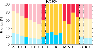
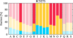
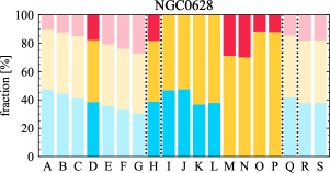
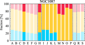
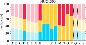
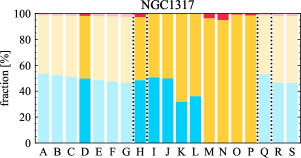
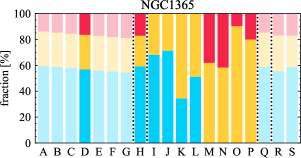
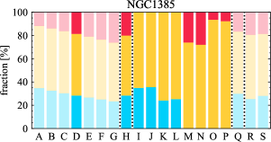
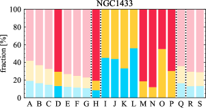
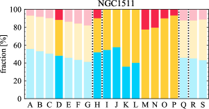
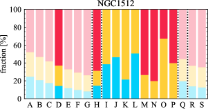
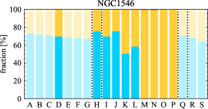
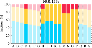
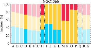
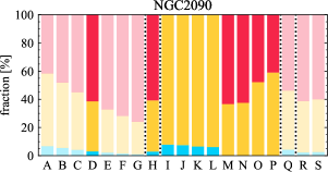
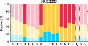
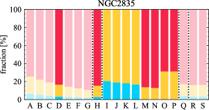
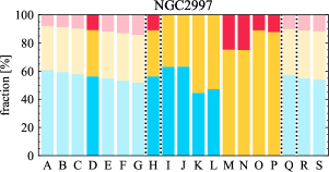
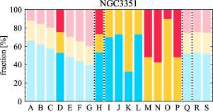

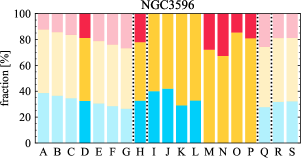
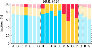
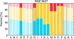
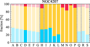
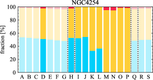
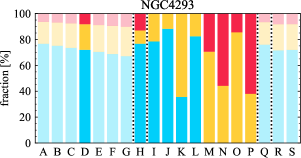
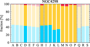
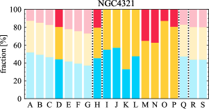
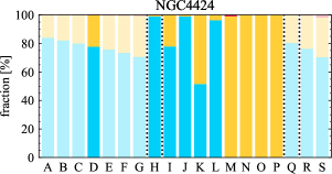
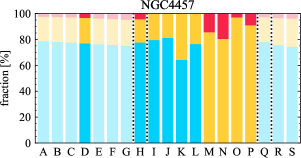
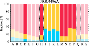
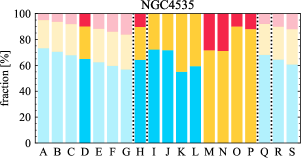
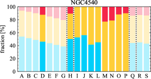
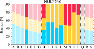
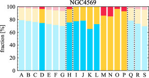
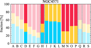
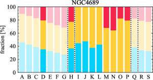
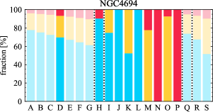
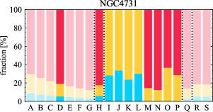
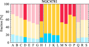
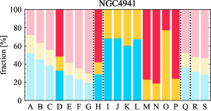
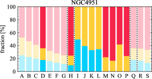
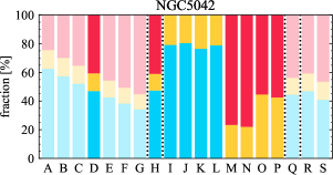
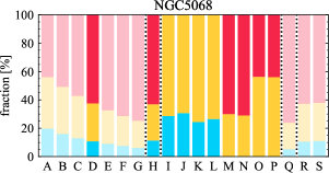
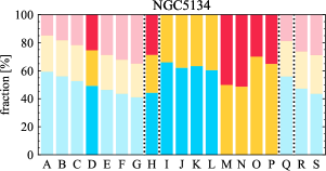
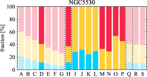
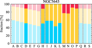
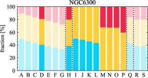
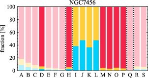
A.4 H Threshold
For a point source at the native resolution of our H data, the effective sensitivity limits in terms of H surface brightness threshold applied to the fiducial maps corresponds to H ii region luminosities () between and erg s-1. Here we carried out two tests to examine the impact of the varying H threshold (which originates from the non-uniform H sensitivity among the sample) on the results.
In the first test, we compare the sight line fractions estimated in the PHANGS-MUSE H images at 150 pc resolution to that measured in the default narrowband images at the same resolution. The PHANGS-MUSE observations are sensitive enough to probe down to H ii regions with 36 erg s-1, about an order of magnitude deeper than the narrowband images. We measure the sight line fractions for the 15 galaxies that have both observations (hereafter overlapping sample). The MUSE images are treated by the same method as the narrowband data for the removal of DIG (see Section 3.1). Namely, the only difference between the two images is the increased sensitivity of the MUSE data.
As an example, Figure A.17 shows the sight line maps for galaxy NGC 0628 based on the narrowband (left) and MUSE (right) images. It can be seen directly that the amount of H-only sight lines increases in the MUSE map as a result of its higher sensitivity. This is accompanied by a decrease in CO-only regions. A direct comparison is provided in Figure A.18. While most galaxies show differences within a factor of two, the difference can be up to a factor 2.5 or even more for those galaxies with the highest (i.e., most shallow narrowband observation). The overlap regions show the least difference between narrowband and MUSE. This is because the fluxes of H emission are higher in overlap regions compared to H-only regions (Section 4.3), so the overlap fraction is less affected by sensitivity.
It is worth noting that the true discrepancy between the MUSE and narrowband sight line fractions are likely smaller than what is obtained here. The low-H-luminosity regions (on the order of 1036-37 erg s-1) are the main source of the discrepancy between the MUSE and narrowband sight line fractions as they are not present in the narrowband observations due to the limited sensitivity. Previous studies on the nature of H-emitting sources in nearby galaxies show that regions ionized by non-H ii sources (e.g., supernova remnants and planetary nebula) tend to have lower H luminosity compared to regions powered by H ii regions (e.g., Belfiore et al., 2016; Hsieh et al., 2017; Pan et al., 2018). The same characteristic is observed in our MUSE data (e.g., Santoro et al. accepted; F. Scheuermann et al. submitted), suggesting that a certain fraction of regions missed by the narrowband observations are not H ii regions888About 30% based on the spectroscopic analysis by Santoro et al. (accepted).. Therefore the discrepancy between the MUSE and narrowband sight line fractions reported here is an upper limit999To be in line with the analysis of narrowband data, for this comparison we did not apply a spectroscopic classification (e.g., like a Baldwin-Phillips-Telervich (BPT) diagram, Baldwin et al., 1981) to the regions identified in the MUSE H map, so the non-H ii regions remain in our DIG-removed MUSE maps. Such a spectroscopic classification is not possible for our narrowband data..
Further we find no correlation between the slight line fractions and global galaxy properties ( and Hubble type) no matter which H image is used, presumably due to the low number of galaxies available in the overlapping sample. Therefore, we carried out a second test to verify whether the trend between the sight line fractions and global galaxy properties (Section 4.1.1) still holds when narrowband is taken into account.
In the second test, we examine the relation between the sight line fractions and global galaxy properties at 150 pc resolution using only galaxies with relatively high narrowband sensitivity (i.e., low ). Specifically, we re-plot Figure 4 using only galaxies with 37.5 erg s-1. Thirty five galaxies satisfy this criterion, the result is shown in Figure A.19. We find good agreement between Figure 4 (full sample) and Figure A.19 for (left panel), although the median fractions can differ by a factor of a few between two samples. For Hubble type, the trends with CO-only and H-only fractions is no longer obvious when only using galaxies with relatively high narrowband sensitivity. This is partially (or perhaps even completely) due to the low-number statistics in the lowest- bin as earlier type galaxies in our sample tend to have less sensitive H images. In spite of that, the median CO-only and H-only fractions of the other two -type bins and the overlap fractions agree well with those derived using the full sample.
In summary, these two tests demonstrate that the H threshold is an important factor in the sight line analysis. Our results remain qualitatively robust once accounting for H threshold, but further confirmation with a high sensitivity and large sample is required in the future.
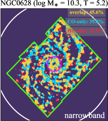
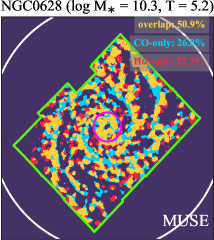
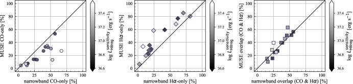
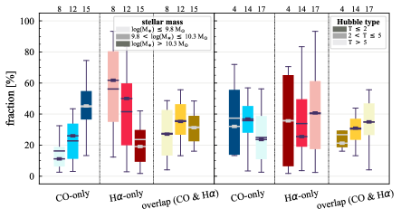
A.5 CO () Threshold
We clip the CO images at our best-matching resolution of 150 pc using a surface density threshold of 10 M☉ pc-2. We test the effect of this threshold by varying the threshold from 7 to 13 M☉ pc-2, % to % with respect to the fiducial threshold. The sight line fractions for a threshold of 7–13 M☉ pc-2 with an interval of 1 M☉ pc-2 are presented in Figure A.16 columns A–G, respectively (column D is the default result of this work).
As somewhat expected, the fractions of CO-only sight lines gradually decrease with increasing threshold in all galaxies, while H-only sight lines gradually increase. The fractions of CO-only sight lines show a decrease within a factor 3 (with a few exceptions) when the threshold varies from % to % with respect to the fiducial threshold. An opposite trend is observed for H-only sight lines, but the magnitude of the change is comparable to that of CO-only sight line. There is no uniform trend between CO threshold and the fraction of overlap sight lines, both increasing and decreasing trends are seen in our galaxies. Nonetheless, the typical magnitude of the change is smaller than for CO-only sight lines, not larger than a factor of 2. This is because the flux of CO in the overlap regions tend to be higher than that in the CO-only regions (and presumably much higher than the applied threshold); therefore they are less sensitive to the choice of the surface density threshold. Overall, we find that the dependence of sight line fractions on the applied threshold is rather uniform across the sample. For this reason, our results remain qualitatively the same when the CO threshold varies by 30%.
Appendix B Sight Line Maps and Fractions for Individual Galaxies at Different Spatial Scales
This appendix presents an atlas of the sight line distributions in our 49 galaxies. Figure B.20 presents galaxy maps showing CO-only (blue), H-only (red), and overlapping CO and H emission (yellow) at spatial resolutions of 150, 300, 500, 1000, and 1500 pc. The sight line fractions measured within 0.6 are listed in Table LABEL:tab_fractions.
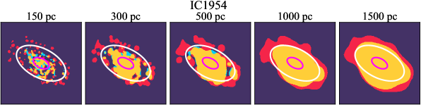
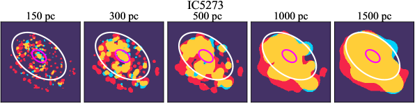
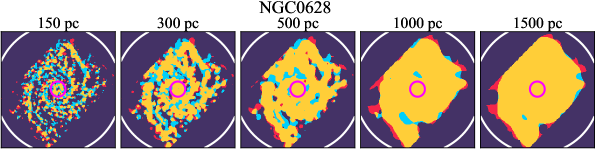
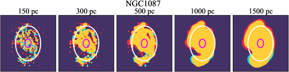
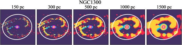
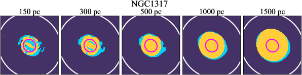
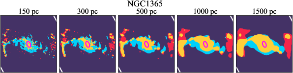
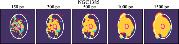
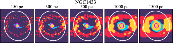
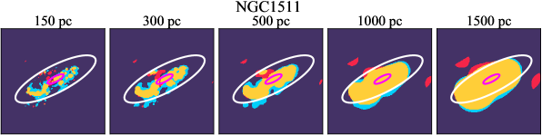
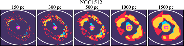
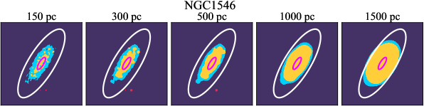
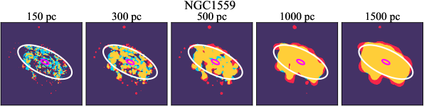
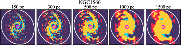
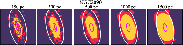
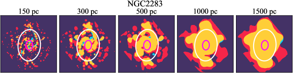
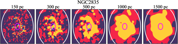
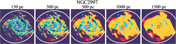
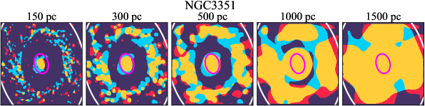
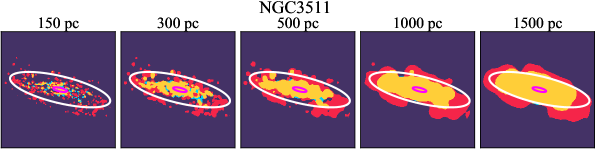
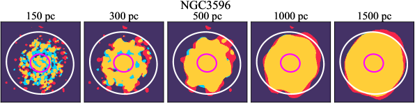
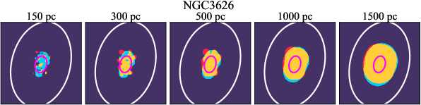
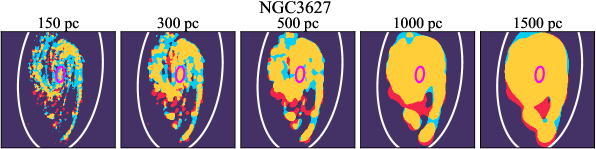
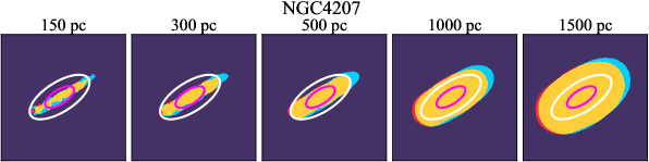
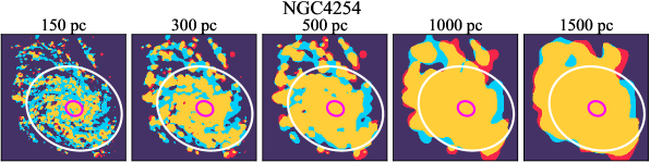
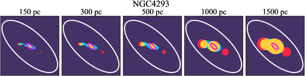
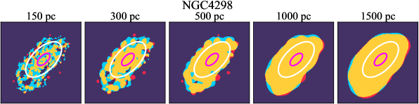
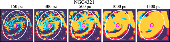
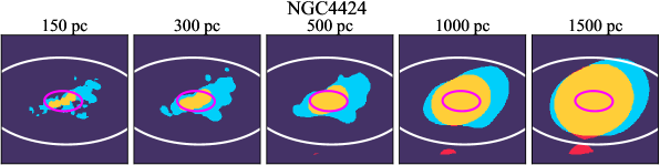
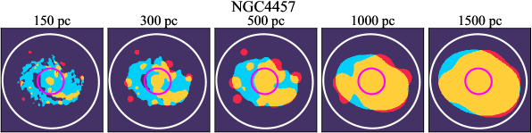
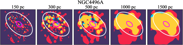
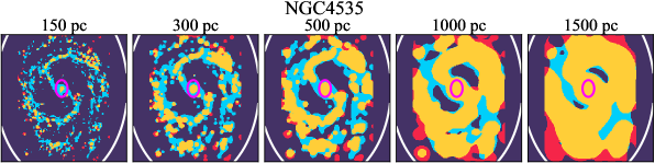
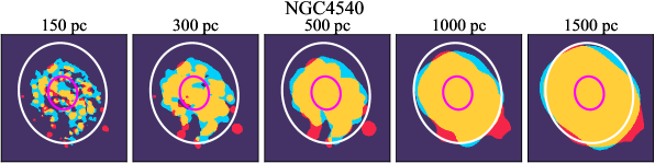
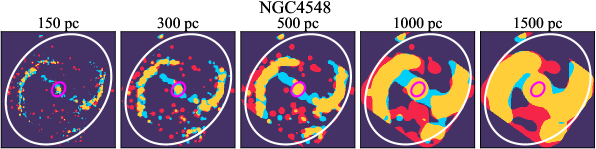
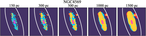
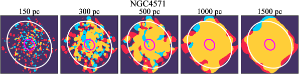
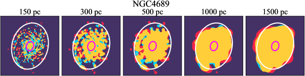
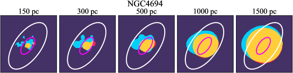
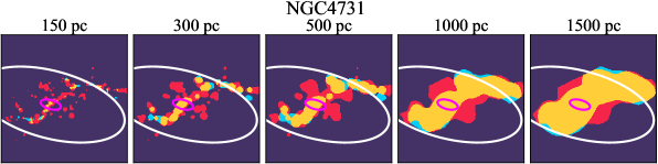
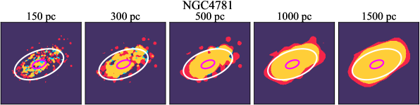
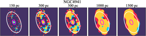
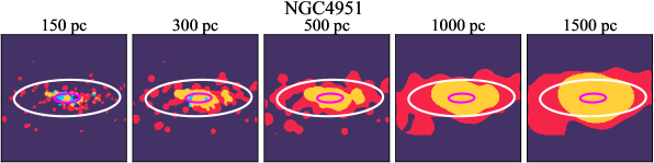
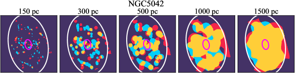
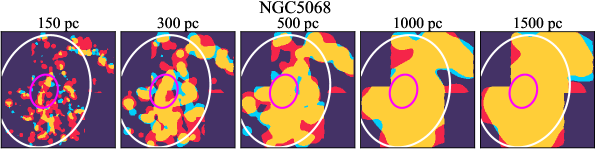
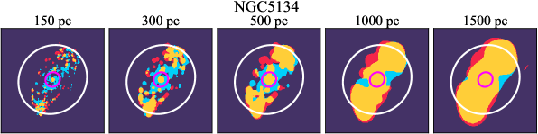
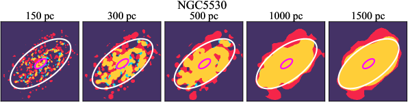
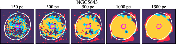
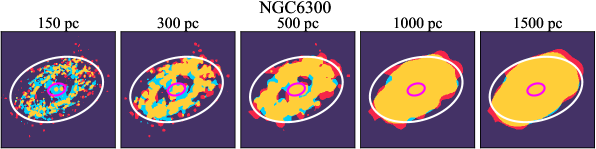
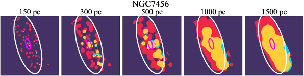
| Galaxy | 150 pc | 300 pc | 500 pc | 1000 pc | 1500 pc |
| IC1954 | (19.3, 34.2, 46.5) | (6.1, 19.2, 74.7) | (3.6, 17.0, 79.3) | (0.0, 4.7, 95.3) | (0.0, 0.0, 100.0) |
| IC5273 | (11.6, 61.0, 27.4) | (8.3, 35.7, 56.1) | (3.9, 23.8, 72.3) | (2.5, 4.9, 92.6) | (1.6, 0.4, 98.1) |
| NGC0628 | (38.5, 17.7, 43.7) | (24.6, 9.6, 65.8) | (13.7, 7.3, 79.0) | (4.8, 7.0, 88.2) | (1.8, 6.6, 91.6) |
| NGC1087 | (23.6, 20.7, 55.6) | (8.1, 12.7, 79.2) | (2.0, 9.3, 88.7) | (0.2, 4.2, 95.6) | (0.1, 1.1, 98.8) |
| NGC1300 | (26.7, 42.1, 31.3) | (14.1, 42.3, 43.6) | (7.8, 41.7, 50.4) | (5.0, 35.8, 59.2) | (4.5, 27.5, 68.0) |
| NGC1317 | (49.8, 1.7, 48.4) | (30.8, 1.2, 68.0) | (23.8, 0.4, 75.8) | (14.4, 0.0, 85.6) | (9.0, 0.1, 90.9) |
| NGC1365 | (56.9, 16.4, 26.7) | (40.7, 23.6, 35.6) | (32.4, 25.9, 41.7) | (24.1, 26.9, 49.0) | (19.8, 26.8, 53.4) |
| NGC1385 | (28.4, 18.7, 52.9) | (12.1, 16.1, 71.8) | (5.7, 12.0, 82.4) | (2.6, 7.8, 89.6) | (2.3, 4.5, 93.3) |
| NGC1433 | (13.3, 70.6, 16.1) | (9.2, 68.1, 22.7) | (8.0, 63.6, 28.4) | (8.4, 51.3, 40.3) | (8.6, 43.0, 48.4) |
| NGC1511 | (48.1, 11.7, 40.1) | (29.8, 10.7, 59.4) | (19.5, 7.6, 73.0) | (6.0, 2.5, 91.6) | (2.4, 0.2, 97.5) |
| NGC1512 | (14.3, 63.0, 22.7) | (11.0, 56.8, 32.2) | (7.2, 54.8, 38.0) | (4.8, 43.6, 51.6) | (4.9, 34.0, 61.1) |
| NGC1546 | (69.7, 0.2, 30.2) | (48.2, 0.2, 51.7) | (36.9, 0.0, 63.0) | (25.1, 0.0, 74.9) | (16.2, 0.0, 83.8) |
| NGC1559 | (50.4, 11.6, 38.0) | (22.9, 10.7, 66.4) | (7.5, 8.8, 83.7) | (0.8, 4.7, 94.4) | (0.2, 2.4, 97.5) |
| NGC1566 | (36.6, 26.5, 36.9) | (22.3, 26.9, 50.8) | (13.7, 28.6, 57.6) | (6.2, 28.9, 64.9) | (3.6, 28.3, 68.1) |
| NGC2090 | (3.0, 61.4, 35.5) | (0.0, 45.8, 54.1) | (0.0, 45.9, 54.1) | (0.0, 33.0, 67.0) | (0.0, 14.7, 85.3) |
| NGC2283 | (11.9, 53.2, 34.9) | (5.2, 29.9, 64.9) | (1.5, 20.1, 78.4) | (0.0, 3.6, 96.4) | (0.0, 0.2, 99.8) |
| NGC2835 | (3.4, 83.4, 13.2) | (2.0, 67.7, 30.3) | (0.7, 61.9, 37.4) | (0.0, 49.9, 50.1) | (0.0, 41.1, 58.9) |
| NGC2997 | (56.2, 10.8, 33.0) | (35.7, 13.2, 51.1) | (22.3, 15.0, 62.7) | (9.5, 16.0, 74.5) | (3.7, 14.6, 81.8) |
| NGC3351 | (52.9, 24.4, 22.7) | (42.3, 17.9, 39.8) | (28.6, 15.7, 55.7) | (16.5, 12.4, 71.1) | (8.2, 8.9, 82.9) |
| NGC3511 | (11.2, 60.1, 28.7) | (5.3, 47.2, 47.4) | (1.5, 41.9, 56.6) | (0.1, 25.1, 74.8) | (0.0, 12.9, 87.1) |
| NGC3596 | (32.5, 18.8, 48.7) | (9.7, 16.9, 73.5) | (1.6, 15.4, 83.0) | (0.1, 11.6, 88.3) | (0.1, 4.1, 95.8) |
| NGC3626 | (71.5, 7.2, 21.3) | (22.0, 14.8, 63.2) | (11.4, 12.3, 76.3) | (8.8, 6.3, 85.0) | (8.2, 3.1, 88.7) |
| NGC3627 | (45.2, 13.3, 41.4) | (27.8, 13.3, 58.9) | (16.1, 12.5, 71.4) | (6.8, 11.2, 82.0) | (4.8, 9.9, 85.2) |
| NGC4207 | (32.4, 6.0, 61.5) | (16.1, 4.0, 79.9) | (7.4, 1.9, 90.7) | (0.0, 0.0, 100.0) | (0.0, 0.0, 100.0) |
| NGC4254 | (50.9, 2.4, 46.7) | (29.5, 1.7, 68.8) | (18.0, 1.1, 80.8) | (8.0, 0.9, 91.2) | (4.8, 0.4, 94.9) |
| NGC4293 | (72.0, 8.2, 19.8) | (52.5, 14.1, 33.4) | (36.5, 20.3, 43.1) | (11.2, 29.0, 59.8) | (1.7, 29.3, 69.1) |
| NGC4298 | (43.4, 2.9, 53.7) | (14.0, 0.6, 85.4) | (2.0, 0.0, 98.0) | (0.0, 0.0, 100.0) | (0.0, 0.0, 100.0) |
| NGC4321 | (44.0, 19.7, 36.3) | (29.1, 17.1, 53.8) | (17.2, 16.7, 66.1) | (5.7, 14.2, 80.1) | (1.8, 11.7, 86.6) |
| NGC4424 | (77.7, 0.2, 22.0) | (74.1, 0.0, 25.9) | (63.6, 0.0, 36.4) | (40.0, 0.1, 59.9) | (24.5, 1.2, 74.3) |
| NGC4457 | (76.9, 3.3, 19.8) | (55.1, 6.4, 38.6) | (35.7, 10.7, 53.5) | (12.7, 10.2, 77.2) | (8.8, 5.8, 85.3) |
| NGC4496A | (6.9, 79.9, 13.2) | (7.9, 54.4, 37.7) | (4.3, 37.5, 58.2) | (1.1, 21.1, 77.8) | (1.0, 13.0, 86.0) |
| NGC4535 | (65.0, 9.9, 25.1) | (50.0, 8.0, 42.0) | (34.1, 8.9, 57.0) | (15.5, 11.9, 72.6) | (10.1, 12.8, 77.1) |
| NGC4540 | (46.3, 12.3, 41.5) | (26.0, 6.7, 67.3) | (14.8, 6.2, 79.0) | (8.6, 4.2, 87.2) | (4.1, 1.9, 94.0) |
| NGC4548 | (37.0, 32.5, 30.5) | (29.4, 28.6, 42.1) | (20.4, 30.5, 49.1) | (12.4, 27.0, 60.6) | (5.2, 19.4, 75.4) |
| NGC4569 | (74.5, 3.6, 21.9) | (52.0, 5.4, 42.7) | (34.3, 5.2, 60.5) | (16.6, 6.9, 76.5) | (10.2, 7.9, 81.9) |
| NGC4571 | (29.7, 48.5, 21.8) | (22.7, 22.9, 54.4) | (10.7, 18.6, 70.7) | (3.5, 8.5, 88.0) | (3.2, 3.9, 92.9) |
| NGC4689 | (35.4, 20.7, 43.9) | (16.5, 14.3, 69.2) | (8.1, 10.2, 81.7) | (1.6, 5.5, 92.9) | (0.3, 2.7, 97.0) |
| NGC4694 | (69.7, 6.8, 23.5) | (62.6, 4.1, 33.3) | (48.8, 3.1, 48.2) | (19.4, 1.4, 79.3) | (6.0, 1.0, 93.0) |
| NGC4731 | (5.4, 81.0, 13.7) | (6.8, 58.6, 34.6) | (6.7, 49.4, 43.9) | (4.0, 32.4, 63.7) | (2.4, 19.1, 78.4) |
| NGC4781 | (14.1, 40.8, 45.2) | (3.9, 27.0, 69.1) | (0.7, 21.4, 77.9) | (0.0, 9.4, 90.6) | (0.0, 0.5, 99.5) |
| NGC4941 | (33.0, 51.7, 15.3) | (27.6, 36.5, 35.9) | (18.5, 30.1, 51.4) | (5.2, 18.6, 76.2) | (2.0, 9.5, 88.5) |
| NGC4951 | (17.9, 64.0, 18.2) | (3.3, 60.7, 36.0) | (0.0, 60.8, 39.1) | (0.0, 39.9, 60.1) | (0.0, 21.9, 78.1) |
| NGC5042 | (47.0, 40.6, 12.4) | (47.9, 26.1, 26.1) | (32.6, 24.1, 43.3) | (12.3, 17.8, 69.9) | (6.4, 11.1, 82.6) |
| NGC5068 | (10.7, 62.5, 26.8) | (12.9, 30.3, 56.7) | (6.4, 17.9, 75.6) | (2.4, 8.2, 89.4) | (0.5, 5.0, 94.5) |
| NGC5134 | (49.2, 25.4, 25.4) | (40.1, 17.3, 42.6) | (26.6, 16.8, 56.6) | (9.1, 13.5, 77.4) | (4.1, 10.4, 85.5) |
| NGC5530 | (11.5, 59.3, 29.2) | (6.3, 33.2, 60.5) | (1.2, 22.5, 76.2) | (0.1, 8.3, 91.7) | (0.0, 1.2, 98.8) |
| NGC5643 | (51.4, 11.2, 37.5) | (30.6, 8.5, 60.9) | (15.6, 6.4, 78.0) | (5.9, 3.5, 90.6) | (3.5, 2.3, 94.2) |
| NGC6300 | (40.6, 19.1, 40.4) | (19.8, 16.4, 63.9) | (8.5, 15.4, 76.1) | (1.7, 8.0, 90.3) | (1.0, 3.4, 95.5) |
| NGC7456 | (2.6, 93.3, 4.1) | (5.6, 72.3, 22.1) | (4.4, 63.4, 32.1) | (1.8, 43.4, 54.8) | (0.6, 29.0, 70.4) |
Appendix C Sight line Fractions versus Properties of Galaxies and Observations
Here we present the scatter plots of galaxy and observational properties against the three sight line fractions in Figure C.21. The properties we explore are (a) stellar mass, (b) Hubble type, (c) galaxy distance, (d) optical size indicated by , (e) disk inclination, (f) effective H ii region sensitivity (log(), Section 3.1, (g) native resolutions of H observation, (h) DIG fraction, (i) effective sensitivity of CO observation (1 sensitivity in at 150 pc resolution), (j) native resolution of CO observation, (k) specific star formation rate sSFR, and (l) offset from the star-forming main sequence MS. Discussion can be found in the main text in Section 4.1.1. Correlation coefficients of each relation shown in Figure C.21 are provided in Table 5 in the main text.

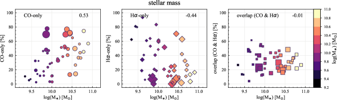
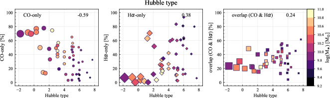
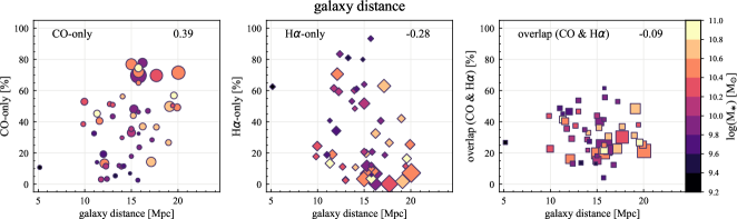

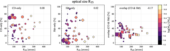
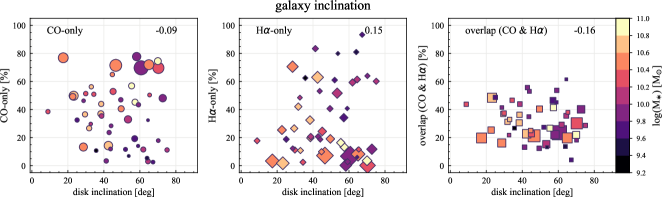
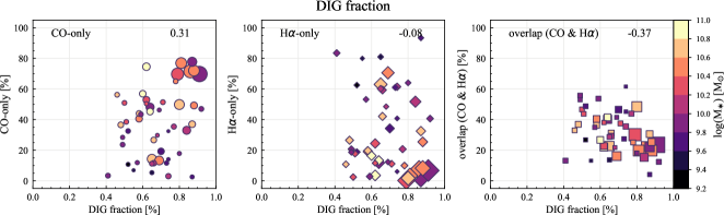
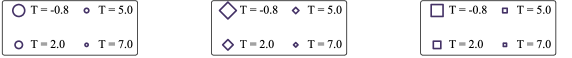
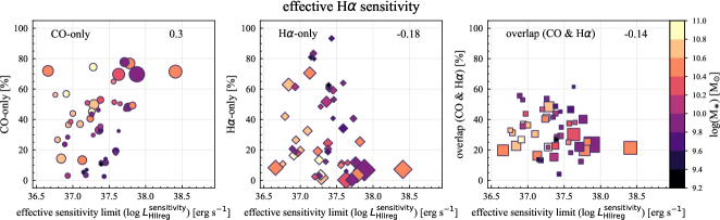
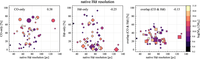
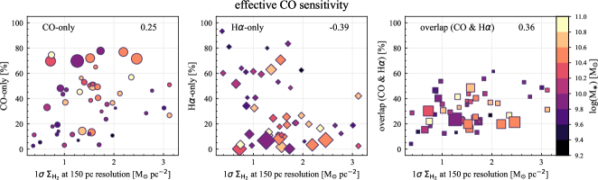

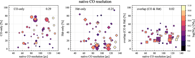
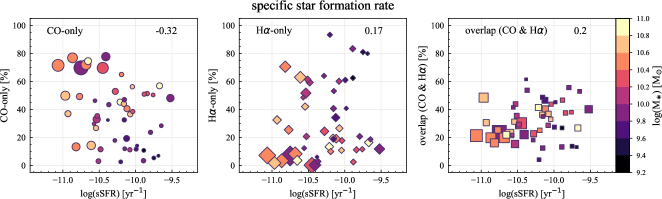
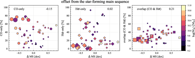
Appendix D Comparison of Cloud Visibility time with Chevance et al.(2020)
Here we directly compare the radial variation in the cloud visibility time derived from our analysis () with the GMC lifetime during which CO is visible () measured by Chevance et al. (2020) for the seven galaxies analyzed in both studies. The results from the two studies are compared in Figure D.22. Overall, the two studies show similar results, particularly in regard to the absolute (or ) for most radial bins. The relative (or ) among different galaxies also shows reasonable agreement. The robustness to the adopted methodology suggests that both results indeed reflect the visibility time of molecular cloud traced by CO emission. Larger discrepancies are seen in regions where the emission (either CO or H) are relatively sparse and/or weak, such as the larger radii and lower galaxy (NGC 5068), suggesting that the sensitivity and completeness of observation are important factors in estimating cloud visibility time.
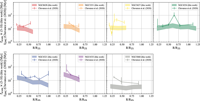
References
- Accurso et al. (2017) Accurso, G., Saintonge, A., Catinella, B., et al. 2017, MNRAS, 470, 4750
- Anand et al. (2021) Anand, G. S., Lee, J. C., Van Dyk, S. D., et al. 2021, MNRAS, 501, 3621. doi:10.1093/mnras/staa3668
- Arimoto et al. (1996) Arimoto, N., Sofue, Y., & Tsujimoto, T. 1996, PASJ, 48, 275
- Asplund et al. (2009) Asplund, M., Grevesse, N., Sauval, A. J., et al. 2009, ARA&A, 47, 481. doi:10.1146/annurev.astro.46.060407.145222
- Azimlu et al. (2011) Azimlu, M., Marciniak, R., & Barmby, P. 2011, AJ, 142, 139
- Baldwin et al. (1981) Baldwin, J. A., Phillips, M. M., & Terlevich, R. 1981, PASP, 93, 5. doi:10.1086/130766
- Barnes et al. (2020) Barnes, A. T., Longmore, S. N., Dale, J. E., et al. 2020, MNRAS, 498, 4906. doi:10.1093/mnras/staa2719
- Barnes et al. (2021) Barnes, A. T., Glover, S. C. O., Kreckel, K., et al. 2021, MNRAS. doi:10.1093/mnras/stab2958
- Battersby et al. (2017) Battersby, C., Bally, J., & Svoboda, B. 2017, ApJ, 835, 263
- Belfiore et al. (2016) Belfiore, F., Maiolino, R., Maraston, C., et al. 2016, MNRAS, 461, 3111. doi:10.1093/mnras/stw1234
- Belfiore et al. (submitted) Belfiore, F., Santoro, F., Groves, B., et al. 2021, arXiv:2111.14876
- Beuther et al. (2017) Beuther, H., Meidt, S., Schinnerer, E., et al. 2017, A&A, 597, A85. doi:10.1051/0004-6361/201526749
- Bigiel et al. (2008) Bigiel, F., Leroy, A., Walter, F., et al. 2008, AJ, 136, 2846
- Blanc et al. (2009) Blanc, G. A., Heiderman, A., Gebhardt, K., et al. 2009, ApJ, 704, 842. doi:10.1088/0004-637X/704/1/842
- Bolatto et al. (2013) Bolatto, A. D., Wolfire, M., & Leroy, A. K. 2013, ARA&A, 51, 207. doi:10.1146/annurev-astro-082812-140944
- Bradley et al. (2006) Bradley, T. R., Knapen, J. H., Beckman, J. E., et al. 2006, A&A, 459, L13
- Brinchmann et al. (2004) Brinchmann, J., Charlot, S., White, S. D. M., et al. 2004, MNRAS, 351, 1151. doi:10.1111/j.1365-2966.2004.07881.x
- Buta et al. (2015) Buta, R. J., Sheth, K., Athanassoula, E., et al. 2015, ApJS, 217, 32. doi:10.1088/0067-0049/217/2/32
- Calzetti et al. (2007) Calzetti, D., Kennicutt, R. C., Engelbracht, C. W., et al. 2007, ApJ, 666, 870. doi:10.1086/520082
- Carles et al. (2016) Carles, C., Martel, H., Ellison, S. L., et al. 2016, MNRAS, 463, 1074. doi:10.1093/mnras/stw2056
- Catinella et al. (2018) Catinella, B., Saintonge, A., Janowiecki, S., et al. 2018, MNRAS, 476, 875. doi:10.1093/mnras/sty089
- Chevance et al. (2020) Chevance, M., Kruijssen, J. M. D., Hygate, A. P. S., et al. 2020, MNRAS, 493, 2872
- Chevance et al. (2022) Chevance, M., Kruijssen, J. M. D., Krumholz, M. R., et al. 2022, MNRAS, 509, 272. doi:10.1093/mnras/stab2938
- Chung et al. (2009) Chung, A., van Gorkom, J. H., Kenney, J. D. P., et al. 2009, AJ, 138, 1741. doi:10.1088/0004-6256/138/6/1741
- Colombo et al. (2014) Colombo, D., Hughes, A., Schinnerer, E., et al. 2014, ApJ, 784, 3. doi:10.1088/0004-637X/784/1/3
- Colombo et al. (2018) Colombo, D., Kalinova, V., Utomo, D., et al. 2018, MNRAS, 475, 1791
- Corbelli et al. (2017) Corbelli, E., Braine, J., Bandiera, R., et al. 2017, A&A, 601, A146
- Crocker et al. (2011) Crocker, A. F., Bureau, M., Young, L. M., et al. 2011, MNRAS, 410, 1197. doi:10.1111/j.1365-2966.2010.17537.x
- Davis et al. (2014) Davis, T. A., Young, L. M., Crocker, A. F., et al. 2014, MNRAS, 444, 3427. doi:10.1093/mnras/stu570
- den Brok et al. (2021) den Brok, J. S., Chatzigiannakis, D., Bigiel, F., et al. 2021, MNRAS, 504, 3221. doi:10.1093/mnras/stab859
- Díaz-García et al. (2020) Díaz-García, S., Moyano, F. D., Comerón, S., et al. 2020, A&A, 644, A38. doi:10.1051/0004-6361/202039162
- Donohoe-Keyes et al. (2019) Donohoe-Keyes, C. E., Martig, M., James, P. A., et al. 2019, MNRAS, 489, 4992. doi:10.1093/mnras/stz2474
- Egusa et al. (2004) Egusa, F., Sofue, Y., & Nakanishi, H. 2004, PASJ, 56, L45. doi:10.1093/pasj/56.6.L45
- Egusa et al. (2009) Egusa, F., Kohno, K., Sofue, Y., et al. 2009, ApJ, 697, 1870. doi:10.1088/0004-637X/697/2/1870
- Ellison et al. (2019) Ellison, S. L., Viswanathan, A., Patton, D. R., et al. 2019, MNRAS, 487, 2491. doi:10.1093/mnras/stz1431
- Emsellem et al. (accepted) Emsellem, E., Schinnerer, E., Santoro, F., et al. 2021, arXiv:2110.03708
- Engargiola et al. (2003) Engargiola, G., Plambeck, R. L., Rosolowsky, E., et al. 2003, ApJS, 149, 343. doi:10.1086/379165
- Feldmann et al. (2011) Feldmann, R., Gnedin, N. Y., & Kravtsov, A. V. 2011, ApJ, 732, 115
- Fitzpatrick (1999) Fitzpatrick, E. L. 1999, PASP, 111, 63. doi:10.1086/316293
- Gaia Collaboration et al. (2018) Gaia Collaboration, Brown, A. G. A., Vallenari, A., et al. 2018, A&A, 616, A1. doi:10.1051/0004-6361/201833051
- González Delgado et al. (2015) González Delgado, R. M., García-Benito, R., Pérez, E., et al. 2015, A&A, 581, A103
- Gratier et al. (2012) Gratier, P., Braine, J., Rodriguez-Fernandez, N. J., et al. 2012, A&A, 542, A108
- Haffner et al. (2009) Haffner, L. M., Dettmar, R.-J., Beckman, J. E., et al. 2009, Reviews of Modern Physics, 81, 969. doi:10.1103/RevModPhys.81.969
- Haydon et al. (2020) Haydon, D. T., Kruijssen, J. M. D., Chevance, M., et al. 2020, MNRAS, 498, 235
- Herrera-Endoqui et al. (2015) Herrera-Endoqui, M., Díaz-García, S., Laurikainen, E., et al. 2015, A&A, 582, A86
- Hilmi et al. (2020) Hilmi, T., Minchev, I., Buck, T., et al. 2020, MNRAS, 497, 933. doi:10.1093/mnras/staa1934
- Hoopes et al. (1999) Hoopes, C. G., Walterbos, R. A. M., & Rand, R. J. 1999, ApJ, 522, 669. doi:10.1086/307670
- Hoopes & Walterbos (2003) Hoopes, C. G. & Walterbos, R. A. M. 2003, ApJ, 586, 902. doi:10.1086/367954
- Hsieh et al. (2017) Hsieh, B. C., Lin, L., Lin, J. H., et al. 2017, ApJ, 851, L24. doi:10.3847/2041-8213/aa9d80
- Hughes et al. (2013) Hughes, A., Meidt, S. E., Colombo, D., et al. 2013, ApJ, 779, 46. doi:10.1088/0004-637X/779/1/46
- Indebetouw et al. (2008) Indebetouw, R., Whitney, B. A., Kawamura, A., et al. 2008, AJ, 136, 1442. doi:10.1088/0004-6256/136/4/1442
- James et al. (2009) James, P. A., Bretherton, C. F., & Knapen, J. H. 2009, A&A, 501, 207
- Jeffreson & Kruijssen (2018) Jeffreson, S. M. R. & Kruijssen, J. M. D. 2018, MNRAS, 476, 3688. doi:10.1093/mnras/sty594
- Jeffreson et al. (2020) Jeffreson, S. M. R., Kruijssen, J. M. D., Keller, B. W., et al. 2020, MNRAS, 498, 385. doi:10.1093/mnras/staa2127
- Jeffreson et al. (2021) Jeffreson, S. M. R., Keller, B. W., Winter, A. J., et al. 2021, MNRAS, 505, 1678. doi:10.1093/mnras/stab1293
- Katz (1992) Katz, N. 1992, ApJ, 391, 502. doi:10.1086/171366
- Kawamura et al. (2009) Kawamura, A., Mizuno, Y., Minamidani, T., et al. 2009, ApJS, 184, 1
- Kelvin et al. (2014) Kelvin, L. S., Driver, S. P., Robotham, A. S. G., et al. 2014, MNRAS, 444, 1647
- Kennicutt (1998) Kennicutt, R. C. 1998, ARA&A, 36, 189
- Kennicutt & Evans (2012) Kennicutt, R. C. & Evans, N. J. 2012, ARA&A, 50, 531
- Kim et al. (2017) Kim, E., Hwang, H. S., Chung, H., et al. 2017, ApJ, 845, 93. doi:10.3847/1538-4357/aa80db
- Kim et al. (2021) Kim, J., Chevance, M., Kruijssen, J. M. D., et al. 2021, MNRAS. doi:10.1093/mnras/stab878
- Klessen & Hennebelle (2010) Klessen, R. S. & Hennebelle, P. 2010, A&A, 520, A17. doi:10.1051/0004-6361/200913780
- Kreckel et al. (2016) Kreckel, K., Blanc, G. A., Schinnerer, E., et al. 2016, ApJ, 827, 103
- Kreckel et al. (2018) Kreckel, K., Faesi, C., Kruijssen, J. M. D., et al. 2018, ApJ, 863, L21
- Kruijssen & Longmore (2014) Kruijssen, J. M. D. & Longmore, S. N. 2014, MNRAS, 439, 3239
- Kruijssen et al. (2018) Kruijssen, J. M. D., Schruba, A., Hygate, A. P. S., et al. 2018, MNRAS, 479, 1866
- Kruijssen et al. (2019) Kruijssen, J. M. D., Schruba, A., Chevance, M., et al. 2019, Nature, 569, 519. doi:10.1038/s41586-019-1194-3
- Lacerda et al. (2018) Lacerda, E. A. D., Cid Fernandes, R., Couto, G. S., et al. 2018, MNRAS, 474, 3727. doi:10.1093/mnras/stx3022
- Laine et al. (2016) Laine, J., Laurikainen, E., & Salo, H. 2016, A&A, 596, A25
- Lang et al. (2020) Lang, P., Meidt, S. E., Rosolowsky, E., et al. 2020, ApJ, 897, 122. doi:10.3847/1538-4357/ab9953
- Lee et al. (2021) Lee, J. C., Whitmore, B. C., Thilker, D. A., et al. 2021, arXiv:2101.02855
- Leroy et al. (2008) Leroy, A. K., Walter, F., Brinks, E., et al. 2008, AJ, 136, 2782
- Leroy et al. (2011) Leroy, A. K., Bolatto, A., Gordon, K., et al. 2011, ApJ, 737, 12
- Leroy et al. (2012) Leroy, A. K., Bigiel, F., de Blok, W. J. G., et al. 2012, AJ, 144, 3
- Leroy et al. (2013) Leroy, A. K., Walter, F., Sandstrom, K., et al. 2013, AJ, 146, 19
- Leroy et al. (2019) Leroy, A. K., Sandstrom, K. M., Lang, D., et al. 2019, ApJS, 244, 24. doi:10.3847/1538-4365/ab3925
- Leroy et al. (2021a) Leroy, A. K., Hughes, A., Liu, D., et al. 2021a, ApJS, 255, 19. doi:10.3847/1538-4365/abec80
- Leroy et al. (2021b) Leroy, A. K., Schinnerer, E., Hughes, A., et al. 2021b, ApJS, 257, 43. doi:10.3847/1538-4365/ac17f3
- Leroy et al. (2021c) Leroy, A. K., Rosolowsky, E., Usero, A., et al. 2021c, arXiv:2109.11583
- Louie et al. (2013) Louie, M., Koda, J., & Egusa, F. 2013, ApJ, 763, 94. doi:10.1088/0004-637X/763/2/94
- Mac Low & Klessen (2004) Mac Low, M.-M. & Klessen, R. S. 2004, Reviews of Modern Physics, 76, 125. doi:10.1103/RevModPhys.76.125
- Martinet & Friedli (1997) Martinet, L. & Friedli, D. 1997, A&A, 323, 363
- McKee & Ostriker (2007) McKee, C. F. & Ostriker, E. C. 2007, ARA&A, 45, 565. doi:10.1146/annurev.astro.45.051806.110602
- McMullin et al. (2007) McMullin, J. P., Waters, B., Schiebel, D., et al. 2007, Astronomical Data Analysis Software and Systems XVI, 376, 127
- Meidt et al. (2009) Meidt, S. E., Rand, R. J., & Merrifield, M. R. 2009, ApJ, 702, 277. doi:10.1088/0004-637X/702/1/277
- Meidt et al. (2013) Meidt, S. E., Schinnerer, E., García-Burillo, S., et al. 2013, ApJ, 779, 45
- Meidt et al. (2018) Meidt, S. E., Leroy, A. K., Rosolowsky, E., et al. 2018, ApJ, 854, 100. doi:10.3847/1538-4357/aaa290
- Menéndez-Delmestre et al. (2007) Menéndez-Delmestre, K., Sheth, K., Schinnerer, E., et al. 2007, ApJ, 657, 790
- Mizuno et al. (2001) Mizuno, N., Rubio, M., Mizuno, A., et al. 2001, PASJ, 53, L45. doi:10.1093/pasj/53.6.L45
- Momose et al. (2013) Momose, R., Koda, J., Kennicutt, R. C., et al. 2013, ApJ, 772, L13
- Oey et al. (2003) Oey, M. S., Parker, J. S., Mikles, V. J., et al. 2003, AJ, 126, 2317
- Oey et al. (2007) Oey, M. S., Meurer, G. R., Yelda, S., et al. 2007, ApJ, 661, 801
- Onodera et al. (2010) Onodera, S., Kuno, N., Tosaki, T., et al. 2010, ApJ, 722, L127
- Pan & Kuno (2017) Pan, H.-A. & Kuno, N. 2017, ApJ, 839, 133. doi:10.3847/1538-4357/aa60c2
- Pan et al. (2018) Pan, H.-A., Lin, L., Hsieh, B.-C., et al. 2018, ApJ, 854, 159. doi:10.3847/1538-4357/aaa9bc
- Pessa et al. (2021) Pessa, I., Schinnerer, E., Belfiore, F., et al. 2021, A&A, 650, A134. doi:10.1051/0004-6361/202140733
- Pettini & Pagel (2004) Pettini, M. & Pagel, B. E. J. 2004, MNRAS, 348, L59
- Pety et al. (2013) Pety, J., Schinnerer, E., Leroy, A. K., et al. 2013, ApJ, 779, 43. doi:10.1088/0004-637X/779/1/43
- Pour-Imani et al. (2016) Pour-Imani, H., Kennefick, D., Kennefick, J., et al. 2016, ApJ, 827, L2. doi:10.3847/2041-8205/827/1/L2
- Querejeta et al. (2019) Querejeta, M., Schinnerer, E., Schruba, A., et al. 2019, A&A, 625, A19. doi:10.1051/0004-6361/201834915
- Querejeta et al. (2021) Querejeta, M., Schinnerer, E., Meidt, S., et al. 2021, arXiv:2109.04491
- Reynaud & Downes (1998) Reynaud, D. & Downes, D. 1998, A&A, 337, 671
- Rosolowsky et al. (2021) Rosolowsky, E., Hughes, A., Leroy, A. K., et al. 2021, MNRAS. doi:10.1093/mnras/stab085
- Rousseau-Nepton et al. (2018) Rousseau-Nepton, L., Robert, C., Martin, R. P., et al. 2018, MNRAS, 477, 4152
- Saintonge et al. (2011) Saintonge, A., Kauffmann, G., Kramer, C., et al. 2011, MNRAS, 415, 32. doi:10.1111/j.1365-2966.2011.18677.x
- Saintonge et al. (2016) Saintonge, A., Catinella, B., Cortese, L., et al. 2016, MNRAS, 462, 1749. doi:10.1093/mnras/stw1715
- Saintonge et al. (2017) Saintonge, A., Catinella, B., Tacconi, L. J., et al. 2017, ApJS, 233, 22. doi:10.3847/1538-4365/aa97e0
- Sakamoto et al. (1994) Sakamoto, S., Hayashi, M., Hasegawa, T., et al. 1994, ApJ, 425, 641. doi:10.1086/174011
- Sakamoto et al. (1997) Sakamoto, S., Hasegawa, T., Handa, T., et al. 1997, ApJ, 486, 276. doi:10.1086/304479
- Sakamoto et al. (1999) Sakamoto, K., Okumura, S. K., Ishizuki, S., et al. 1999, ApJ, 525, 691
- Salim et al. (2007) Salim, S., Rich, R. M., Charlot, S., et al. 2007, ApJS, 173, 267. doi:10.1086/519218
- Sánchez et al. (2012) Sánchez, S. F., Kennicutt, R. C., Gil de Paz, A., et al. 2012, A&A, 538, A8. doi:10.1051/0004-6361/201117353
- Sánchez et al. (2014) Sánchez, S. F., Rosales-Ortega, F. F., Iglesias-Páramo, J., et al. 2014, A&A, 563, A49
- Sánchez et al. (2019) Sánchez, S. F., Barrera-Ballesteros, J. K., López-Cobá, C., et al. 2019, MNRAS, 484, 3042
- Santoro et al. (accepted) Santoro, F., Kreckel, K., Belfiore, F., et al. 2021, arXiv:2111.09362
- Schaye et al. (2015) Schaye, J., Crain, R. A., Bower, R. G., et al. 2015, MNRAS, 446, 521. doi:10.1093/mnras/stu2058
- Schinnerer et al. (2013) Schinnerer, E., Meidt, S. E., Pety, J., et al. 2013, ApJ, 779, 42
- Schinnerer et al. (2019) Schinnerer, E., Hughes, A., Leroy, A., et al. 2019, ApJ, 887, 49
- Schlafly & Finkbeiner (2011) Schlafly, E. F. & Finkbeiner, D. P. 2011, ApJ, 737, 103. doi:10.1088/0004-637X/737/2/103
- Schmidt (1959) Schmidt, M. 1959, ApJ, 129, 243. doi:10.1086/146614
- Schruba et al. (2010) Schruba, A., Leroy, A. K., Walter, F., et al. 2010, ApJ, 722, 1699
- Schruba et al. (2011) Schruba, A., Leroy, A. K., Walter, F., et al. 2011, AJ, 142, 37
- Schruba et al. (2012) Schruba, A., Leroy, A. K., Walter, F., et al. 2012, AJ, 143, 138
- Schruba et al. (2019) Schruba, A., Kruijssen, J. M. D. & Leroy, A. K. 2019, ApJ, 883, 2
- Sheth et al. (2005) Sheth, K., Vogel, S. N., Regan, M. W., et al. 2005, ApJ, 632, 217
- Sun et al. (2020a) Sun, J., Leroy, A. K., Ostriker, E. C., et al. 2020, ApJ, 892, 148
- Sun et al. (2020b) Sun, J., Leroy, A. K., Schinnerer, E., et al. 2020, ApJ, 901, 8
- Teyssier (2002) Teyssier, R. 2002, A&A, 385, 337. doi:10.1051/0004-6361:20011817
- Tomičić et al. (2017) Tomičić, N., Kreckel, K., Groves, B., et al. 2017, ApJ, 844, 155. doi:10.3847/1538-4357/aa7b30
- Tomičić et al. (2019) Tomičić, N., Ho, I.-T., Kreckel, K., et al. 2019, ApJ, 873, 3. doi:10.3847/1538-4357/ab03ce
- Tomičić et al. (2021) Tomičić, N., Vulcani, B., Poggianti, B. M., et al. 2021, ApJ, 907, 22. doi:10.3847/1538-4357/abca93
- Utomo et al. (2018) Utomo, D., Sun, J., Leroy, A. K., et al. 2018, ApJ, 861, L18. doi:10.3847/2041-8213/aacf8f
- Verley et al. (2007) Verley, S., Combes, F., Verdes-Montenegro, L., et al. 2007, A&A, 474, 43
- Walter et al. (2008) Walter, F., Brinks, E., de Blok, W. J. G., et al. 2008, AJ, 136, 2563. doi:10.1088/0004-6256/136/6/2563
- Whitmore et al. (2011) Whitmore, B. C., Chandar, R., Kim, H., et al. 2011, ApJ, 729, 78
- Wilson (1995) Wilson, C. D. 1995, ApJ, 448, L97
- Wolfire et al. (2010) Wolfire, M. G., Hollenbach, D., & McKee, C. F. 2010, ApJ, 716, 1191. doi:10.1088/0004-637X/716/2/1191
- Yajima et al. (2021) Yajima, Y., Sorai, K., Miyamoto, Y., et al. 2021, PASJ. doi:10.1093/pasj/psaa119
- Zhang et al. (2017) Zhang, K., Yan, R., Bundy, K., et al. 2017, MNRAS, 466, 3217. doi:10.1093/mnras/stw3308
- Zurita et al. (2004) Zurita, A., Relaño, M., Beckman, J. E., et al. 2004, A&A, 413, 73