The extremely young planetary nebula M 3-27: an analysis of its evolution, physical conditions and abundances
Abstract
Spectrophotometric data of the young planetary nebula M 3-27, from 2004 to 2021, are presented and discussed. We corroborate that the H i Balmer lines present features indicating they are emitted by the central star, therefore He i lines were used to correct line fluxes by effects of reddening. Important variability on the nebular emission lines between 1964 to 2021, probably related to density changes in the nebula, is reported. Diagnostic diagrams to derive electron temperatures and densities have been constructed. The nebula shows a very large density contrast with an inner density of the order of 107 cm-3 and an outer density of about cm-3. With these values of density, electron temperatures of K have been found from collisionally excited lines. Due to the central star emits in the H+ lines, ionic abundances relative to He+ were calculated from collisionally excited and recombination lines, and scaled to H+ by considering that He+/H+ He/H. ADF(O+2) values were also determined. Total abundance values obtained indicate sub-solar abundances, similarly to what is found in other comparable objects like IC 4997.
keywords:
planetary nebulae: individual: M 3-27 – ISM: abundances – ISM: kinematics and dynamics1 Introduction
Planetary nebulae (PNe) are formed by the ejection of parts of the stellar atmosphere during advanced stages of evolution of low-intermediate mass stars. The ejecta, initially neutral or molecular, expands at velocities of about 1020 km s-1 and later it is photoionized by the energetic photons of the star when it evolves from the Asymptotic Giant Branch (AGB) phase towards higher effective temperatures and reaches temperatures larger than 25,000 K. The stellar transition between the post-AGB and the PN phase is not well known, it is not smooth and substantial photometric and spectral changes might occur in few years.
There are few stars known to be in this transition period, presenting very young planetary nebulae. Some of them are IC 4997, the Stingray nebula, VV 8, PM 1-322, and a few others.
In this work, we analyse spectrophotometric data of the very young and compact PN M 3-27 whose interesting behaviour has been studied since 50 years ago (Kohoutek, 1968; Adams, 1975; Ahern, 1978; Barker, 1978; Feibelman, 1985; Miranda et al., 1997; Wesson et al., 2005). The main characteristics of M 3-27 are listed in Table 1. Previous works showed the presence of two density zones inside the nebula, an inner zone of 106 cm-3 and a compact outer zone of 10104 cm-3.
Given the high density of the nebula, it has been difficult to determine a proper value of using plasma line diagnostics. Ahern (1978) estimated a value of K by comparing the line ratios of [O iii]5007 and [Ne iii]3869 according to the methodology presented by Ahern (1975). Wesson et al. (2005) determined a K using the line ratio [O iii] 4959/4363 by assuming a density cm-3, estimated from high-order H i Balmer lines.
By means of position-velocity diagrams (PVD), Miranda et al. (1997) studied the line profiles and kinematics of this object. They found that the H line has a kinematic profile different than those of [S ii] and [N ii] lines. H shows a double peak, much more intense in the red than in the blue, and wide wings extending up to 1500 km s-1, possible due to Rayleigh-Raman dispersion111Rayleigh and Raman scattering are processes of photon scattering by atoms or molecules. Lee & Hyung (2000) and Arrieta & Torres-Peimbert (2003) suggested that the main mechanism of formation of very broad wings on H lines in young planetary nebulae is the Raman scattering of near-Ly photons produced by a dense atomic H i region near to the central star. However, photons may suffer a series of Raman and Rayleigh scattering (in which an incident H photon is scattered as another H photon) before leaving this dense neutral region. occurring in a very dense zone near the central star. In addition, faint H emission can be traced up to about 12 arcsec from the stellar position, which is not shown by the heavy element lines. These latter lines and radio continuum emission at 3.6 cm are originated in a compact inner shell not spatially resolved (FWHM 1.4 arcsec). Miranda et al. (1997) estimated a kinematic age lower than 580 yr for the inner shell of this young PN.
| Names | Gal. coord. | RA (2000) | Dec (2000) | Size | Parallax (mas) | (LSR) | Comments |
|---|---|---|---|---|---|---|---|
| (deg) | (hr:min:s) | (deg:min:sec) | Gaia DR3 | (km s-1) | |||
| PN G043.6+11.6 | 43.3554 +11.698 | 18:27:48 | +14:29:06 | Stellar | 0.1468a | 24b | Wide H |
| IRAS 18255*14.27 | Double peak H i lines | ||||||
| a Gaia Collaboration et al. (2016, 2023) b Miranda et al. (1997) | |||||||
We have studied this object as part of a project devoted to analyse young and dense PNe, whose first results were published by Ruiz-Escobedo & Peña (2022). The general purpose of the project is to determine physical conditions and chemical composition of these young nebulae, with special emphasis in determining the Abundance Discrepancy Factors (ADF) between measurements from collisionally excited lines (CELs) and recombination lines ORLs222The ADF is defined as the ratio of the abundance derived from ORLs to the abundance derived from CELs: ADF(X+i) X / X..
This paper is organized as follows: In §1 we present the introduction with the general characteristics of M 3-27. In §2, observations and data reduction are described. In §3 we analyse the calibrated line intensities to determine reddening corrections based He i lines and analyse the temporal variations of line intensities. In §4 the line profiles are analysed. In §5 physical conditions and chemical abundances from collisionally excited lines and from recombination lines are determined and discussed. Line profiles and kinematics of the plasma are discussed in §6. In §7 we present the discussion of our results and our conclusions can be found in §8.
2 Observations
Spectrophotometric data of M 3-27 were obtained at the Observatorio Astronómico Nacional San Pedro Mártir (OAN-SPM) at Baja California, México, between the years 2004 to 2022. Two spectrographs of different resolution, attached to the 2.1-m telescope, were used: the Boller & Chivens (B&Ch) spectrograph of low-medium dispersion (resolution R () of 685 at 5000 Å) and the REOSC-Echelle spectrograph of high dispersion (resolution R 16,00018,000 at 5000 Å). The log of observations is presented in Table 2.
| Obs. date | Spectrograph(a) | #exp | Slit size | spectral resolution | range | Binning | Airmass | |
| (s) | Å/pix | R(5000Å) | Å | pixpix Å | (average) | |||
| 22/04/2004 | B&Ch (300 l mm | 2 60 | 5’4" | 2.23 | 567 | 34507400 | 22 7.00.35 | 1.04 |
| 25/04/2004 | REOSC-Echelle | 2 900 | 13.3”4" | 0.34 | 16,000 | 36006800 | 22 0.30.35 | 1.13 |
| 30/06/2019 | REOSC-Echelle | 3 1800 | 13.3”2" | 0.30 | 18,000 | 36007200 | 11 0.20.18 | 1.05 |
| 04/05/2021 | B&Ch (600 l mm-1) | 3 900 | 5’4" | 1.54 | 685 | 38005950 | 22 5.40.35 | 1.07 |
| 05/05/2021 | B&Ch (600 l mm-1) | 2 900 | 5’4" | 1.54 | 685 | 52007300 | 22 5.40.35 | 1.07 |
| 06/05/2021 | B&Ch (300 l mm-1) | 2 300 | 5’4" | 2.23 | 567 | 34507400 | 22 7.00.35 | 1.24 |
| 02/10/2021 | REOSC-Echelle | 3 1800 | 13.3"4" | 0.34 | 16,000 | 36007200 | 22 0.30.35 | 1.25 |
| 16/08/2022 | REOSC-Echelle | 3 1800 | 13.3"2" | 0.30 | 18,000 | 3600–7200 | 11 0.20.18 | 1.28 |
| (a) The P.A. of the slit for B&Ch observations was always E-W, for all REOSC-Echelle it was E-W, except for 2021 when it was N-S. | ||||||||
| (b) In parenthesis, the grating used. | ||||||||
2.1 Data reduction
iraf 333iraf is distributed by the National Optical Observatory, which is operated by the Associated Universities for Research in Astronomy, Inc., under contract to the National Science Foundation. tasks were used for data reduction. The 2D B&Ch frames were bias subtracted and flat fielded. Spectra were extracted (extraction window width included all the observed flux) and wavelength and flux calibrated. A Cu-Ar lamp, observed after each exposure, was used for wavelength calibration of B&Ch observations. The standard stars Feige 34, Feige 66 and BD+30 2642 were observed each night for flux calibration with a slit width of 500 m (6.6 arcsec), in order to include all the stellar flux.
2D REOSC-Echelle spectra were bias subtracted but no flat fielding was applied. Spectra were extracted from all the available orders, the extraction window included all the flux. Wavelength calibration was applied with a Th-Ar lamp obtained after each scientific observation. Standard stars from the list by Hamuy et al. (1992) were observed for flux calibration.
All observations were also corrected by effects of atmospheric extinction, using the curve determined by Schuster & Parrao (2001) for the OAN-SPM sky.
Calibrated spectra of different epochs have been used to determine variations of the emission lines, to analyse the line profiles, to determine the reddening, the physical conditions and the nebular ionic and total abundances. Fluxes from available lines in each spectrum were measured using iraf’s splot task and normalized to the flux of H (H). Errors in line fluxes were estimated following Tresse et al. (1999) procedure. For REOSC-Echelle spectra, FWHM (full width at half-maximum) were also measured and corrected by effects of instrumental and thermal broadening (assuming the electron temperature derived in each observation), subtracted in quadrature from the measured FWHM. For physical conditions and abundances, errors were estimated using Monte Carlo simulations, a set of 400 random points was generated following a normal distribution centred on each observed line intensity.
3 Reddening correction
In very high-density ionized gas, when the nebula is optically thick to H Lyman series and partially thick to H Balmer series, particularly thick to H, the photons will be self-absorbed and will reappear in a cascade as P, H and Ly photons. Thus the H photons emitted will increase and H photons will decrease, increasing the observed H/H intensity ratio. Then such a ratio is not useful to determine the reddening. Capriotti (1964) calculated the theoretical values of the Balmer series in case of self-absorption for different optical depths. We have used Capriotti’s procedure to determine c(H) for the different observations presented in the literature (Kohoutek, 1968; Adams, 1975; Ahern, 1978; Barker, 1978, and ours in this paper) finding that the c(H) value seems to vary with time, increasing from 0.500.75 for the observations of the seventies to values larger than 1.351.95 in the years from 2004 to 2021, due to the changes in H/H value probably produced by changes in the emission of the central star.
Due to the above, we consider that such a procedure is not appropriate to determine the external reddening for the OAN-SPM observations. Instead we decided to determine it by using the He i lines following the procedure recently proposed by Zamora et al. (2022). Such a procedure consists in using the intensities of the optical He i singlet lines 4922, 6678, 7281 and the triplet 5876 line, relative to 6678, because their theoretical intensities are unaffected by optical depth and density effects, even for densities as large as 108 cm-3, contrary to what occurs with other He i triplet lines (Rodríguez, 2020; Zamora et al., 2022).
The expression used to calculate c(H) is:
| (1) |
where are the observed fluxes, are the de-reddened fluxes, and is the extinction law given by Cardelli et al. (1989), assuming a ratio of total to selective extinction . The reference wavelength () is 6678 Å, which corresponds to the most intense of the He i singlet lines. This line will be used to normalize the line intensities.
By using PyNeb Luridiana et al. (2015), the theoretical intensities were calculated for a density of 107 cm-3 and a temperature of 104 K, the atomic parameters used are those by Porter et al. (2012, 2013).
The ratios of He i observed fluxes and dereddened fluxes for all the observations from 2004 to 2021, normalized to the line 6678 Å as said above, and their values of were plotted in the plane vs. (see Fig. 1). A linear regression was applied to all the plots, deriving in each case the c(H) value which is the slope of the calculated lines.


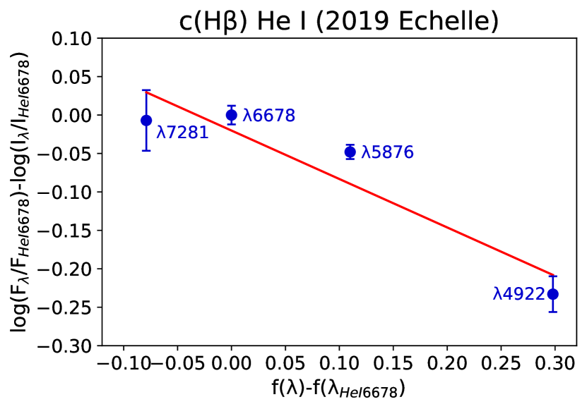
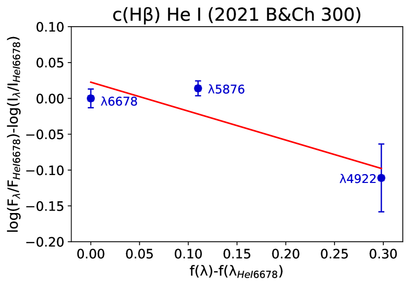


The results are presented in Table 3 where the RMS of the regression is adopted as the error for the determined c(H). The value R2 of the regression is given. For each observation, the c(H) values derived this way were used to deredden the spectra.
| Year | Obs | c(H) | RMS | R2 | He i observed lines |
|---|---|---|---|---|---|
| 2004 | B&Ch (300 l/mm) | 0.47 | 0.02 | 0.95 | 4922, 5876, 6678, 7281 |
| 2004 | REOSC-Echelle | 0.42 | 0.04 | 0.66 | 4922, 5876, 6678 |
| 2019 | REOSC-Echelle | 0.63 | 0.03 | 0.89 | 4922, 5876, 6678, 7281 |
| 2021 | B&Ch (300 l/mm) | 0.40 | 0.03 | 0.79 | 4922, 5876, 6678 |
| 2021 | B&Ch (600 l/mm) | 0.46 | 0.04 | 0.72 | 4922, 5876, 6678, 7281 |
| 2021 | REOSC-Echelle | 0.48 | 0.05 | 0.63 | 4922, 5876, 6678 |
The observed and dereddened fluxes relative to H and the FWHM of all the detected lines, for all the observations, are presented in a table on-line. In Table 4 we present an example of such a table.
| Ion | Fλ/F(H) | Fλ) | Iλ/I(H) | Iλ) | FWHM | ||||
|---|---|---|---|---|---|---|---|---|---|
| (Å) | (Å) | (Å) | (km s-1) | (km s-1) | |||||
| H25 | 3669.47 | 3668.66 | 0.28 | 0.11 | 0.46 | 0.19 | 0.23 | 9.59 | 66.35 |
| H24 | 3671.48 | 3670.67 | 0.51 | 0.17 | 0.83 | 0.27 | 0.26 | 10.79 | 66.31 |
| H23 | 3673.76 | 3672.90 | 0.61 | 0.27 | 0.97 | 0.43 | 0.52 | 21.31 | 70.27 |
| H22 | 3676.37 | 3675.50 | 0.73 | 0.21 | 1.17 | 0.34 | 0.71 | 28.99 | 70.71 |
| H21 | 3679.36 | 3678.50 | 0.96 | 0.22 | 1.53 | 0.36 | 0.22 | 9.15 | 70.41 |
| H20 | 3682.81 | 3681.92 | 1.13 | 0.27 | 1.80 | 0.43 | 0.41 | 16.87 | 72.13 |
| H19 | 3686.83 | 3686.03 | 1.31 | 0.39 | 2.10 | 0.62 | 0.33 | 13.38 | 65.22 |
| H18 | 3691.56 | 3690.68 | 1.06 | 0.36 | 1.68 | 0.58 | 0.25 | 10.25 | 71.39 |
| H17 | 3697.15 | 3696.39 | 1.81 | 0.51 | 2.88 | 0.81 | 0.49 | 20.08 | 61.39 |
| H16 | 3703.86 | 3703.03 | 2.12 | 0.48 | 3.40 | 0.77 | 0.59 | 23.79 | 66.94 |
| He i | 3705.04 | 3704.10 | 0.92 | 0.35 | 1.47 | 0.57 | 0.52 | 20.88 | 75.75 |
| H15 | 3711.97 | 3711.14 | 2.21 | 0.31 | 3.54 | 0.50 | 0.76 | 30.71 | 66.72 |
| H14+[S iii] | 3721.83 | 3720.94 | 4.01 | 0.34 | 6.41 | 0.56 | 0.69 | 27.79 | 72.10 |
| O ii] | 3726.03 | 3725.28 | 0.48 | 0.11 | 0.76 | 0.18 | 0.36 | 14.51 | 60.75 |
| O ii] | 3728.82 | 3728.08 | 0.29 | 0.11 | 0.46 | 0.17 | 0.84 | 33.88 | 59.58 |
| H13 | 3734.37 | 3733.52 | 3.12 | 0.26 | 4.95 | 0.43 | 0.73 | 29.21 | 67.92 |
| H12 | 3750.15 | 3749.34 | 3.84 | 0.55 | 6.07 | 0.88 | 0.80 | 31.95 | 64.84 |
| H11 | 3770.63 | 3769.81 | 4.37 | 0.30 | 6.80 | 0.49 | 0.42 | 16.52 | 64.96 |
| a : observed flux, : error, : dereddened flux, : error, : expansion velocity, | |||||||||
| : heliocentric velocity. The complete table, including all the observations, is on-line-material. | |||||||||
3.1 Temporal variations of line intensities
Fig. 2 shows the temporal evolution of some important lines in the period from 1964 to 2021. The data from 1964 to 1978 were obtained from Kohoutek (1968); Adams (1975); Ahern (1978) Barker (1978). In Fig. 2 (up, left) the evolution of lines [O iii]5007, 4363 and [Ne iii]3869 relative to H are presented. It is observed that the nebular line [O iii]5007 diminished by a factor of 2.7 in this period, while the auroral line [O iii]4363 and the [Ne iii]3869 line do not show significant variations. This is a consequence of the critical density () that is lower for 5007 than for the other lines (see Table 5). In the case of H i Balmer lines (Fig. 2 (up, right)) impressive changes are found, the H/H ratio increased by a factor of 4 in the period of 50 years, from during 1970 to in 2021, while H and H show no significant variations relative to H. This confirms that H is partially emitted by the central star and its variations can be attributed to changes in the stellar emission.
The behaviour of other heavy element lines is shown in Fig. 2 (low, left) where the most large variation is presented by [O ii]3727+ nebular lines (the addition of [O ii]3726 and 3729 lines) which decreased by a factor of 4 in the period from 1970 to 2020, from in 1970 to in 2020, while the [O ii] 7325+ auroral lines (the addition of [O ii]7319, 7320, 7329,and 7330 lines) show small variations. Other lines present smaller changes. He i 5876 increased by a factor of 1.4 in 2004 while [S ii] 6717 did not vary significantly. In Fig. 2 (low, right) the behaviour of [N ii] 6584 nebular line and 5755 auroral line are shown, in this case the nebular line 6584 had varied significantly while the auroral line 5755 presents small changes.
All the above is an effect of the critical densities that are lower for the lines [O ii]3727+ and [N ii]6584 than for the others. The critical densities derived from PyNeb for the lines mentioned here are tabulated in Table 5. The atomic parameters used are listed in Table 12, and the temperature assumed was 17,000 K which is an average value of the temperatures derived for the different observations (see Table 6).
As H i lines show characteristics indicating they are emitted by the stellar atmosphere and present variations through time, we also analysed the evolution of line intensities relative to He i 5876 line, which is emitted by the nebula. In Figure 3, we present the temporal evolution of the intensities of the same lines analysed above but normalized to the mentioned He i line. For the observations from the 1970s, the He i 5876 line is only reported in the data from Ahern (1978) and Barker (1978), however the line intensities show the same behaviour as it was found for the normalization to H, highlighting the suppression of the emission of nebular lines of [O ii], [N ii] and [O iii].


| Ion | a | |
|---|---|---|
| (Å) | (cm-3) | |
| O ii] | 3726 | 4.9710 |
| O ii] | 3729 | 1.4310 |
| O ii] | 7325 | 4.9210 |
| O iii] | 4363 | 3.0610 |
| O iii] | 5007 | 8.1510 |
| N ii] | 5755 | 1.9510 |
| N ii] | 6584 | 1.0910 |
| Ne iii] | 3869 | 1.3310 |
| S ii] | 6717 | 1.4410 |
| S ii] | 6731 | 3.8910 |
| S ii] | 4068 | 2.2210 |
| Ar iii] | 5191 | 5.0610 |
| Ar iii] | 7136 | 6.9210 |
| Ar iv] | 4711 | 1.9610 |
| Ar iv] | 4740 | 1.2010 |
| Ar iv] | 7170 | 2.1610 |
| Cl iii] | 5518 | 7.3410 |
| Cl iii] | 5538 | 4.0110 |
| a Critical densities calculated with PyNeb | ||
| using atomic data presented in Appendix C. | ||
4 The lines profiles
In Fig. 4 the line profiles of H, H, [O iii]4959 and He i 5876 are shown from the 2019 high resolution REOSC-Echelle observations. It is found that both H i lines show double peak with a faint component appearing to the blue. The red component is very intense in comparison with the blue one. Both peaks are separated by about 70 km s-1. Such a profile was already found by Miranda et al. (1997) who reported that H exhibits a type III P-Cygni profile with two emissions at 84 and 7 km s-1, separated by an absorption at 55 km s-1. In addition H shows very extended wings traced up to 1500 km s-1. We have found this profile in all the Balmer lines at least up to H. The H i line profiles are different from the profiles of He i and heavy element lines which show a unique peak at a systemic velocity of km s-1 as shown in Fig. 4. Such peak coincides better with the position of the absorption shown by the Balmer lines, which indicates that the Balmer lines originate mainly in a different zone than the He i and the heavy element lines, most probably in the atmosphere of the central star. This will complicate the calculus of abundances as it will be seen in the next sections.

An interesting fact found in this work is that the line profile of H seems to have changed with time (see Fig. 5). In particular, the blue component of the profile was more intense in 2004 than it was in the period 2019 to 2022. The observations reported by Miranda et al. (1997), obtained in 1993, also shows a blue component similar to the ones of the 20192022 period, with an intensity of about 0.2 the value for the red component. However Tamura et al. (1990) shows a single profile for H from observations obtained by K. M. Shibata previous to 1988.

5 Physical conditions and chemical abundances
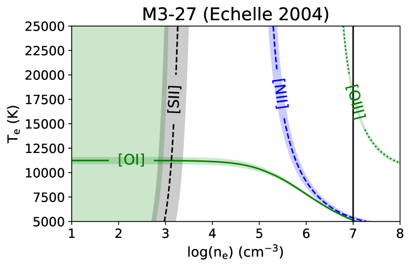
Physical conditions, and , were calculated using PyNeb (Luridiana et al., 2015). This was done by adopting the line intensities relative to H presented in Table 4, determined including all the observed emission (in the case of H i Balmer lines both components were included), corrected by reddening and using the atomic data presented in Table 12. Several plasma diagnostic intensity ratios from the collisionally excited lines (CELs) of different ions are available to determine electron temperature and densities. The behaviour of these diagnostic lines can be observed in the diagnostic diagrams (Figure 6), which were constructed using PyNeb for OAN-SPM observations between 2004 and 2021.
The diagnostic diagrams show that the “traditional” auroral-nebular line intensity ratios normally used to determine electron temperature, such as [O iii](5007+4959)/4363, [N ii](6584+6548)/5755 and [Ar iii] 7136/5192, cannot be used with such a purpose in M 3-27 due to such ratios are more indicative of the electron density. A density of the order of cm-3, higher than the critical density of some nebular lines, are derived from these ratios. On the other hand, the [S ii] 6731/6716 and [O ii] 3729/3726 intensity ratios indicate a much lower density ( cm-3). It is clear from such diagrams that M 3-27 has a large density contrast, being much denser in the inner zone.
The contribution of recombination to the intensity of the nebular line [N ii] 5755 was determined using the relation proposed by Liu et al. (2000), which requires the calculation of the recombination abundance of N+2 (see Tab. 8). This contribution was calculated to be for the REOSC-Echelle observations.
Thus, the determination of an electronic temperature from the CELs of M 3-27 by using the “traditional” method, based on the intersection of a density sensitive line diagnostic with a temperature sensitive line diagnostic, is not possible. To estimate the , we decided to use a methodology similar to the one presented by Wesson et al. (2005) for the analysis of this same object: by assuming a density cm-3, (as estimated from our diagnostic diagrams, as explained above), is determined from the [O iii] (5007+4959)/4363 line ratio. Although it is possible to determine a from [O i] (6364+6300)/5577 line ratio, this value was not used because it corresponds to an outer and neutral zone of the nebula where the gas is not ionized. In Fig. 6 cm-3 is plotted as a vertical solid black line and by using PyNeb getTemden routine the value for was computed. This was applied to each OAN-SPM observations and the respective was assumed for the whole nebula, for each observation.
Physical conditions from optical recombination lines (ORLs) were also determined for some of the observations. The temperature from H i Balmer Jump (BJ) was only determined for the REOSC-Echelle 2019 data, following the procedure given by Liu et al. (2001). However, the derived value is very uncertain and was not used for further calculations.
The temperature from He i was determined from the line ratio 7281/6678 using the relation given by Zhang et al. (2005), which is based on the Benjamin et al. (1999) atomic parameters 444(He i) can be determined also using Porter et al. (2012, 2013) atomic data and PyNeb. We performed such a calculation, obtaining a temperature slightly higher that does not affect the abundance results. Therefore, we kept the value derived with Zhang et al. (2005) method.. (He i) could only be determined for Boller & Chivens observations from 2004 (300 l mm-1) and 2021 (600 l mm-1) and REOSC-Echelle 2019, while for the other observations, the 7281 line was outside the wavelength range of the spectra.
The (He i) was adopted for the recombination lines of heavy elements. O ii density was determined from the 4649/4661 line ratio only for REOSC-Echelle 2019 spectrum.


In Table 6, the values of temperature and density from CELs and ORLs are listed for the different epochs of observation. The more complete data correspond to the REOSC-Echelle 2019 observations, where electron temperatures from CELs have values from 11,100 K for [O i] to 16,800 K for [O iii] and electron densities go from a few thousand cm-3 for the outer zone to several times 107 cm-3 in the inner zone. As expected, He i temperatures, with values between K, are lower than the temperatures derived from CELs. The values listed in this table will be used to determine ionic abundances.
| Parameter/Obs. | Line ratio | B&Ch 2004 (300) | Echelle 2004 | Echelle 2019 | B&Ch 2021 (300) | B&Ch 2021 (600) | Echelle 2021 |
|---|---|---|---|---|---|---|---|
| [O i] | (6364+6300)/5577 | ||||||
| [Ar iii]* | 7136/5192 | — | — | — | 28,420:: | ||
| [O iii]* | (5007+4959)/4363 | — | |||||
| Adopted | Unique zone | — | |||||
| [N i] | 5200/5198 | — | — | — | — | ||
| [O ii] | 3729/3726 | — | — | — | — | ||
| [S ii] | 6731/6716 | ||||||
| [Cl iii] | 5538/5518 | — | — | — | — | — | |
| [S ii]b | (6716+6731)/4068 | — | — | — | |||
| [N ii] () | (6584+6548)/5755 | — | — | — | |||
| [Ar iv]b ) | 7170/4740 | — | — | — | — | — | |
| Adopted | Outer zone | ||||||
| Inner zone | |||||||
| H i (BJ) | — | — | — | 11,500:: | — | 62803210 | — |
| He i | 7281/6678 | — | — | — | |||
| O ii | 4649/4661 | — | — | — | — | — |
5.1 Ionic and total abundances
Given that the H i Balmer lines seem to be emitted partially by the star, it is inadequate to calculate the chemical abundances following the usual procedure, with the emission line intensities relative to H. However, considering that previous authors have calculated the chemistry in M 3-27 by following the usual procedure we decided to calculate ionic and total abundances relative to H+ and the results are shown in Appendix A. These calculations were performed using the routine get.IonAbundance from PyNeb. It is clear that these results are not confident due to the contamination by the central star but we include them here for comparison and for completeness.
In the following section ionic abundances are calculated relative to the He+. Line intensities normalized to He i 5876, which is undoubtedly emitted by the nebula, are used. The lines used to derive ionic abundances are listed in Table 7. Ionic abundances relative to He+ will be escalated to H+ by assuming a value for the He+/H+ abundance ratio and in further sections, total abundances will derived.
| X+i | Lines (Å) |
|---|---|
| N+ | [N ii] 6548, 6584, 5755 |
| O+ | [O ii] 3727+, 7325+ |
| O+2 | [O iii] 4959, 5007, 4363 |
| Ne+2 | [Ne iii] 3868, 3967 |
| S+ | [S ii] 6716, 6731, 4068 |
| S+2 | [S iii] 6312 |
| Cl+2 | [Cl iii] 5517, 5537 |
| Ar+2 | [Ar iii] 5192, 7136 |
| Ar+3 | [Ar iv] 4711,4740, 7170 |
| Fe+ | [Fe ii] 7155 |
| Fe+2 | [Fe iii] 4659, 4701, 4755 |
5.1.1 Ionic abundances relative to He+
To determine ionic abundances relative to He+ we used the data of REOSC-Echelle 2019 and B&Ch 2021 (300 l mm-1), which are the most complete spectra of those obtained at OAN-SPM. As said above, the line intensities were normalized to the intensity of He i 5876. Ionic abundance of elements relative to He+ can be calculated using the next expression:
| (2) |
Here is the emissivity of the line used to calculate the abundance, is the emissivity of the He i line derived using the physical conditions previously determined for He i, and is the line intensity relative to He i 5876. Line emissivities were calculated by using PyNeb getEmissivity task.
Following this method, ionic abundances from CELs relative to He+ were derived by assuming a unique value for given by the [O iii] line diagnostic and two density zones as presented in Table 6. For the once ionized species and Fe+2 the [S ii] was used except in the case of N+, for which 106 cm-3 was adopted as derived by the line ratio [N ii] . A density of 107 cm-3 was used for the twice or more ionized species.
Ionic abundances from the recombination lines of the ions O+2, N+2 and C+2, relative to He+, were computed in the same way and by assuming the and derived from recombination lines. The used was the (He i), while (O ii) determined from the 2019 REOSC-Echelle data was assumed in all cases. C+2 abundance was derived from C ii 4267, O+2 abundance was obtained from the lines of multiplet V1 and N+2 abundance was derived from multiplet V3 lines.
The lines used to determine ionic abundances are those listed in Table 7. The derived ionic abundances are presented in Table 8.
From the ionic abundances relative to He+ ( in Table 8), ionic abundances relative to H+ can be calculated by assuming that M 3-27 is a galactic disc PN with He/H = 0.11 (Kingsburgh & Barlow, 1994) and that He/H = He+/H+, that is, we assume that there is neither He0 nor He+2 present in the nebula. In this way, the ionic abundances relative to H+ were calculated as:
| (3) |
Their values are listed in Table 8. In this table we can appreciate that O+2 is the most abundant ion of oxygen, being 2 or 3 orders of magnitude larger than O+ calculated from 3727+ lines (this is not the case of the O+ abundance derived from the 7325+ lines of the B&Ch 2021 data which is only one order of magnitude lower than O+2). For the ions [N ii], [O iii], [Ar iii] and [Ar iv] the abundances derived from the auroral and trans-auroral lines are similar indicating that used and densities are correct.
The ionic abundances obtained this way can be compared to the values derived directly from H+ (Appendix A). This comparison reveals that the ionic abundances from CELs, , are a factor of 1.2 lower than the values derived by using the H lines , possibly due to the assumption that . This assumption is one of those that produces large uncertainties in the abundances derived here. If we consider than He/H 0.127, the ionic abundances derived from He+ and from H+ would be the same. This He/H value is at standard deviation of the mean of the distribution calculated by Kingsburgh & Barlow (1994) for non-Type I galactic disc PNe, which is He/H 0.1120.015.
The ionic abundances derived from ORLs have diminished by a larger factor when they are compared to the ionic abundances calculated directly by using H line, . This has consequences in the calculus of the ADF(O+2), presented in the same Table, which diminishes from 6.04 (Appendix A) to 3.26.
| Ion | Echelle 2019 | B&Ch 2021 (300) | Ion | Echelle 2019 | B&Ch 2021 (300) |
|---|---|---|---|---|---|
| ORLs | |||||
| He+ 5876 Å | 1 | 1 | He+ 5876 Å | 0.11 | 0.11 |
| O+2 4638 Å () | — | O+2 4638 Å () | — | ||
| O+2 4641 Å () | — | O+2 4641 Å () | — | ||
| O+2 4649 Å () | — | O+2 4649 Å () | — | ||
| O+2 4661 Å () | — | O+2 4661 Å () | — | ||
| O+2 4676 Å () | — | O+2 4676 Å () | — | ||
| O+2 V1 () | — | O+2 V1 () | — | ||
| C+2 4267 Å () | — | C+2 4267 Å () | — | ||
| N+2 5679 Å () | — | N+2 5679 Å () | — | ||
| N+2 V3 () | — | N+2 V3 () | — | ||
| CELs | |||||
| O+ Neb. () | — | O+ Neb. () | — | ||
| O+ Aur. () | — | O+ Aur. () | — | ||
| O+2 Neb. () | O+2 Neb. () | ||||
| O+2 Aur. () | O+2 Aur. () | ||||
| N+ Neb. () | N+ Neb. () | ||||
| N+ Aur. () | N+ Aur. () | ||||
| Ne+2 () | Ne+2 () | ||||
| Ar+2 Neb. () | Ar+2 Neb. () | ||||
| Ar+2 Aur. () | — | Ar+2 Aur. () | — | ||
| Ar+3 Neb. () | — | Ar+3 Neb. () | — | ||
| Ar+3 Aur. () | — | Ar+3 Aur. () | — | ||
| S+ Neb. () | S+ Neb. () | ||||
| S+ T-aur. () | — | S+ T-aur. () | — | ||
| S+2 () | S+2 () | ||||
| Cl+2 () | — | Cl+2 () | |||
| Fe+ () | — | Fe+ () | — | ||
| Fe+2 () | — | Fe+2 () | — | ||
| ADF(O+2) | — | ADF(O+2) | — | ||
5.2 Total abundances
Total abundances of O/H, N/H, Ne/H, Ar/H, S/H, and Cl/H were computed from the ionic abundances (relative to He+ and scaled to H+) and employing the Ionization Correction Factors, ICFs, by Kingsburgh & Barlow (1994). The ICF by Liu et al. (2000) was used for Cl/H abundance 555ICFs allow to correct total abundances for the presence of unseeing ions and the expressions used to obtain total abundance calculations are presented in Appendix B.. The derived abundance values are listed in Table 9, in units of 12+log(X/H). Also the elemental abundances relative to O are listed. The N/H values marked with :: are extremely uncertain due to the large ICFs used.
| Echelle 2019 | B&Ch 2021 (300) | |
|---|---|---|
| He/H | 11.04 | 11.04 |
| O/H | ||
| N/H | 9.79:: | |
| ICF(N) (KB94) | 2568:: | |
| Ne/H | ||
| ICF(Ne) (KB94) | 1 | |
| Ar/H | ||
| ICF(Ar) (KB94) | 1 | 1.87 |
| S/H | ||
| ICF(S) (KB94) | ||
| Cl/H | — | |
| ICF(Cl) (LS00) | — | |
| N/O (KB94) | 1.55:: | |
| Ne/O (KB94) | ||
| Ar/O (KB94) | ||
| S/O (KB94) | ||
| Cl/O (LS00) | — |
6 Expansion velocities from lines
Kinematic analysis from CELs and ORLs was performed for the data from REOSC-Echelle spectra, as these data offer the best spectral resolution (R 18,000) and cover a large range of wavelengths. For this analysis, the FWHMs of lines were measured and corrected by the effect of thermal and instrumental broadening. For the correction by thermal broadening the electron temperature adopted for each observation (as presented in Table 6) was used.
The FWHMs, expansion velocities (determined from FWHM of lines) and radial velocities of the observed lines in the three REOSC-Echelle spectra (2004, 2019 and 2021) are presented as online material together with the line fluxes and intensities for these observations. See an example of these data in Table 4. In Fig. 7 (left) we present the diagram of expansion velocities in function of ionization potentials for different CELs and ORLs (CELs represented by blue points, ORLs by red diamonds, green points correspond to CEL aurorals); it was constructed using REOSC-Echelle data from 2019 because this spectrum presents the largest number of measured lines. This diagram is equivalent to plot vs. distance to the central star, as it is expected that, due to the ionization structure of the nebula, ions more highly ionized are located nearer the central star (see e.g., the work by Peña et al., 2017, and references therein).


In Fig. 7 (left) it is observed that lines of [S ii], [N ii] and [S iii] show velocities larger than 25 km s-1, while lines of [Fe iii] and [O ii] show smaller but have large error bars. Lines of [Ar iii] and [O iii] present of 25 and 21 km s-1 and ions of larger ionization potentials like [Ne iii] and [Ar iv] have the lowest of 20 and 18 km s-1 respectively, thus CELs present a decreasing , from 26 to 18 km s-1, with increasing ionization potential. On the other hand, recombination lines show lower from about 15 to 19 km s-1 which could be interpreted as if recombination lines are originated in a different zone than CELs, however the uncertainties are large, therefore the differences in velocities are not conclusive.
Also in Fig. 7, the green dots represent the of CELs auroral and transauroral lines of [S ii], [N ii], [O iii], [Ar iii] and [Ar iv], which show a different kinematic behaviour between both lines. It is observed that auroral (transauroral) lines of [S ii], [N ii] and [Ar iii] show lower than their respective nebular lines, by about 7, 6 and 6 km s-1, respectively; however, for auroral and nebular lines of [O iii] and [Ar iv] this difference is within the errors bars. This difference can be attributed to the suppression of nebular lines emission due to of these lines is lower than the , which, as it was shown in previous sections, increases in inner parts of the nebula. In this way, in Fig. 7 (right) the differences in of nebular, auroral, and transauroral lines of the same ion are presented as a function of their critical densities. It is clear that lines with higher critical densities show lower .
7 Discussion
The young PN M 3-27 presents several peculiarities that make difficult to perform a classical nebular analysis. The first problem is that the H i lines show P-Cygni type profiles with wide wings, these profiles are different in shape and in kinematic than the He i and heavy element profiles. This indicates that the H i lines are mainly emitted by the central star. We found that H intensity has increased importantly between 1974 to 2004, suggesting important changes in the stellar emission in a period of 50 years.
In addition, several nebular line intensities have changed in the same period. To follow this evolution, the line intensities relative to H were analysed (see Fig. 2), but considering that H is mainly emitted by the central star and might be changing, the line intensities relative to He i 5876 (which has a nebular profile) were also analysed (see Fig. 3). It is found that the line intensities of [O iii]5007, [N ii]6584 and [O ii]3727+ have decreased significantly, while the auroral lines [O iii]4363, [N ii]5755, [O ii]7325+ and also [Ne iii]3869 present some small variations without important changes. This can be interpreted as a suppression of some nebular lines due to the large electron density in the inner nebular zone, with a value of about 107 cm-3 which is in the limit or above the critical density of these lines. This value of , estimated by the [O iii] line ratio is one order of magnitude larger than the value reported in the works by Adams (1975); Ahern (1978); Barker (1978) and Kohoutek (1968) of 106 cm-3, estimated using the same line ratio.
We do not attribute the changes of line intensities to recombination of the nebula because we do not find neither the diminution of the line intensities of high ionization species, like [Ne iii]3869 or the auroral line [O iii]4363, nor the increase of intensities of low ionization species lines, as [N ii]5755 or [O ii]7325+. Instead, the suppression of intensities is observed in lines having the lower critical densities.
Because of the details presented by H i lines, to determine the interstellar logarithmic reddening, c(H), we used a procedure based on the He i lines which provides a value between 0.39 and 0.63 in agreement with values derived by other authors from data of 1970 and calculated considering self-absorption, . It is interesting to note that Schlegel et al. (1998) and Schlafly & Finkbeiner (2011) have reported that the interstellar extinction in M 3-27 direction is c(H)=0.31, therefore a part of the value derived for M 3-27 may be intrinsic in the nebula.
The estimates of electron density and temperature from CELs are complicated by the fact that density present a large contrast, with a value of about 103 cm-3 in the outer zone, and about 107 cm-3 in the inner zone. This high inner value causes that the line ratios usually employed to determine electron temperatures are now sensitive to density. With this density values of temperature between 16,000 and 18,000 K are found for our data. We adopted these values to derived ionic abundances of these observations from the CELs. It should be noted that Wesson et al. (2005) derived K assuming the same density for the inner zone. This occurred because the [O iii]4363 intensity used by them (obtained in the year 2001) is lower than our value and the values reported for the seventies.
The electron temperature can also be determined from the recombination lines of He i, obtaining values of K. Only for REOSC-Echelle 2019 data a temperature from the H i Balmer continuum with a value of 11,500 K was derived, nevertheless, this value is very uncertain and was not used for other calculations. It was found that the temperatures from ORLs are lower than the temperature from CELs, which is an expected result for planetary nebulae (this was first noticed by Peimbert, 1971).
Another difficulty in M 3-27 analysis is the determination of total abundances from CELs. Even though the determination of total O/H abundance is simple (just by adding O+ and O+2 ionic abundances) due to O+ abundance from [O ii]3727+ lines is 3 or 4 orders of magnitude smaller than O+2 abundance (see Table 10), ICFs for other elements that depend on O+, such as N and S, will be severely affected. For REOSC-Echelle spectra, this effect is evident for the ICF(N) by Kingsburgh & Barlow (1994), which would be extremely elevated () and therefore N/H total abundance would be very uncertain and overestimated. An alternative is to determine this ICF by using the auroral lines [O ii] 7325+, as it was done for the B&Ch spectra, in such a case the N/H abundance behaves accordingly to values of disc PNe. However, it is necessary to be cautious in the use of the N abundance derived using [O ii] 7325+ lines because, as it is well known, ionic abundances determined using this auroral line of O+ are systematically larger than the derived from the nebular line (see e.g., Rodríguez, 2020). Along with this problem is the diminution of O+ nebular line intensity in a short period of time. For ICFs for Ar and Ne by Kingsburgh & Barlow (1994), their values are 1 for REOSC-Echelle observations, because they are based on O+2/O rates; in the case of Ar, in REOSC-Echelle spectra Ar+3 is detected and so the correction is made considering the presence of this ion; for Boller & Chivens spectra this ion is not detected and, therefore, the correction was made using the ICF by Kingsburgh & Barlow (1994) that considers only the Ar+2 abundance.
The C abundance derived from the recombination line 4267 is similar to the value reported by Wesson et al. (2005) from the same recombination line. These authors also derived C+2/H+ from the ultraviolet line 1909 intensity and adopting K, their derived value is similar to their value from 4267 and would suggest an ADF(C+2) near 1. Previously Feibelman (1985) had estimated the C+2/H+ value from the same line [C iii]1909 but adopting K. Both C+2/H+ values are very different due to the large dependence of CELs in temperature. Feibelman’s value is more confident and would imply an ADF(C+2) of 1.86, more in agreement to the value derived for O+2 and other elements.
Considering that H i lines seems to be emitted by the star, we have calculated the ionic abundances relative to the He+ for the observations of REOSC-Echelle 2019 and B&Ch 2021, and transformed them to abundances relative to H+ by assuming that He/H = He+/H+ = 0.11. When possible, the ionic abundances derived from the auroral and nebular lines were computed to compare their values.
With this procedure the chemical abundances derived from CELs diminish by a factor of 1.2, while the chemical abundances derived from ORLs diminish by a factor of 2, when compared with the abundances derived relative to H+ (see Appendix A). This effect could be due to the assumptions of and made to determine the emissivity of He+ and the assumption made considering that He+/H+ = He/H, that is, we consider that there is no He0 in the nebula. To determine the contribution He0 to He/H abundance is problematic and still is an open problem (see the discussion presented by Delgado-Inglada et al., 2014). This decrease in abundances has effects on the determination of the ADF(O+2) which is 7.30 when abundances relative to H+ are used (the average value from REOSC-Echelle spectra) and 3.26 if abundances relative He+ are used (from REOSC-Echelle 2019 spectrum).
From the physical conditions and abundances derived from CELs and ORLs there are indications of the existence of two different plasmas in M 3-27 although the kinematics of CELs and ORLs are not so conclusive in this sense.
Our results so far are affected by the complexity of the abundance analysis in M 3-27. We consider that the best values of ionic abundances are those estimated relative to He+ despite the several assumptions that were done for the He+ abundance. Because of the problems for the ICFs that are based in O+ abundance, we consider that the best values for total abundances are those derived with B&Ch 2021 data.
M 3-27 shares similar characteristics with the also young and compact PNe Vy 2-2 and IC 4997 that were analysed in our previous work (Ruiz-Escobedo & Peña, 2022). These three PNe present a large density gradient showing an outer low-density zone with cm-3 and an inner high-density zone with cm-3, being M 3-27 the nebula with the largest gradient. The three objects have sub-solar metallicities and show differences between the of nebular and auroral (or trans-auroral) lines of CELs of ions like [S ii], [N ii], [O iii], [Ar iii] and [Ar iv]. It is very possible that, as it was suggested by Zhang & Liu (2002), the standard temperature diagnostic ratios trend to overestimate of the dense planetary nebulae resulting in an underestimation of total abundances.
Another important similarity between M 3-27 and IC 4997 is the variability of their line intensities and their physical conditions in short periods of time. Kostyakova & Arkhipova (2009) monitored the spectral evolution of IC 4997 for forty years. They claimed that increased by a factor of 5, and increased from 12,000 K to 14,000 K in a period of 20 yr while the nebular ionization degree has been growing with time. The central star seems to have increased its effective temperature from K to 47,000 K in the same period, thus the nebular variations could be produced by changes in the central star which has been heating with time. IC 4997 also present a wide H line with a FWZI equivalent to 5,100 km s-1 attributed to Raman scattering (Arrieta & Torres-Peimbert, 2003). In addition Hyung et al. (1994), from observations, found that H exhibits a P-Cygni profile. Nonetheless, Miranda et al. (2022) showed that during 2019 and 2020, the H profile exhibited only a single-peak profile and that its broad wings narrowed by a factor of 2.
Due to the above exposed, we consider that M 3-27 is an object very similar to IC 4997, in a previous evolutionary stage.
8 Conclusions
From high- and medium-spectral resolution obtained at OAN-SPM, México, from 2004 to 2021, we have analysed the characteristics of the young and dense PN M 3-27. During this epoch the central star shows profiles in emission type P-Cygni in the H i Balmer lines, in particular in H, H, H and H, indicating the presence of a stellar wind. The stellar emission is variable as deduced mainly from the H emission. Due to the stellar emission of the Balmer lines, they cannot be used for determining c(H) from the Balmer decrement, alternatively the He i lines were used and a value of about 0.47 was obtained (see Tab. 3).
M 3-27 is a very dense PN with an inner zone with density about 107 cm-3, which is larger than several critical densities of some nebular lines. This make difficult to determine electron temperatures with the usual nebular-auroral line intensity ratios. By adopting a density of 107 cm-3 as derived from our diagnostic diagrams, a between K was derived from CELs and employed for the calculus of ionic abundances. The inner density value seems to have increased in a period of 30 years from 106 cm-3 in the seventies (Adams, 1975; Ahern, 1978; Barker, 1978; Kohoutek, 1968) to 107 cm-3, value found in this work.
Total abundances in M 3-27 were derived by calculating ionic abundances relative to He+ scalated to H+, and by using the ICFs by Kingsburgh & Barlow (1994) and Liu et al. (2000). The values obtained for 12+log(O/H) are sub-solar, between 8.23 and 8.30 (the solar value is as derived by Asplund et al. 2009). Our derived values for 12+log(O/H) are smaller than the value presented by Wesson et al. (2005), probably due to the lower temperature used by these authors for abundance determinations. Total abundances of elements derived using ICFs based on O+ nebular line 3727+ seem to be overestimated, due to the suppression of this line, so we adopted the total values determined using the auroral line 7325+. The abundance values of other elements relative to O indicate that M 3-27 is a disc nebula (Kingsburgh & Barlow, 1994).
We have analysed the characteristics of M 3-27 in comparison with the also young and compact PNe Vy 2-2 and IC 4997 which also present a large density gradient and variability of their line intensities. In particular M 3-27 is very similar to IC 4997 which has also showed stellar P-Cygni profile, nebular variations and wide H wings attributable to Raman scattering.
In the case of M 3-27, the important variations found on the H intensity suggest important changes on the central star emission. The variation of H profile, from the single-peaked profile reported by Tamura et al. (1990) to the P-Cygni profile, first reported by Miranda et al. (1997) and also found in our work, suggest that the stellar wind has strengthened. This changes in the stellar emission are reflected in the nebula, where it is found an increase in from cm-3 (in the seventies) to cm-3 (after the year 2000) and the consequent suppression on the emission of lines with lower than the of the nebula. Probably the stellar temperature has been changing with time too, however, this parameter was not explored in this work.
Forthcoming observations are needed to analyse the evolution of line intensities and nebular and stellar parameters of this very young planetary nebula, which has showed important changes in its characteristics in short periods of time.
Acknowledgements
This work received partial support from Dirección General de Asuntos del Personal Académico-Programa de Apoyo a Proyectos de Investigación e Innovación Tecnológica (DGAPA-PAPIIT) IN111423, IN105020 and IN103519 and Consejo Nacional de Ciencia y Tecnología (CONACyT), México, project A1-S-15140. FR-E acknowledges scholarship by CONACyT, México. Helpful discussion and suggestions by Dr. Michael G. Richer are deeply acknowledged.
This work is based upon observations carried out at the Observatorio Astronómico Nacional at the Sierra San Pedro Mártir (OAN-SPM), Baja California, México. We thank the daytime and night support staff at the OAN-SPM for facilitating and helping to obtain our observations. The observations during 2021 were obtained by the resident astronomers at OAN-SPM as observers were not allowed at the observatory due to the COVID19 pandemic, so we are particularly grateful to them for their effort.
This work has made use of data from the European Space Agency (ESA) mission Gaia (https://www.cosmos.esa.int/gaia), processed by the Gaia Data Processing and Analysis Consortium (DPAC, https://www.cosmos.esa.int/web/gaia/dpac/consortium). Funding for the DPAC has been provided by national institutions, in particular the institutions participating in the Gaia Multilateral Agreement.
Data Availability
The data underlying this article will be shared on reasonable request to the corresponding author.
References
- Adams (1975) Adams T. F., 1975, ApJ, 202, 114
- Ahern (1975) Ahern F. J., 1975, ApJ, 197, 635
- Ahern (1978) Ahern F. J., 1978, ApJ, 223, 901
- Arrieta & Torres-Peimbert (2003) Arrieta A., Torres-Peimbert S., 2003, ApJS, 147, 97
- Asplund et al. (2009) Asplund M., Grevesse N., Sauval A. J., Scott P., 2009, ARA&A, 47, 481
- Barker (1978) Barker T., 1978, ApJ, 219, 914
- Bautista et al. (2015) Bautista M. A., Fivet V., Ballance C., Quinet P., Ferland G., Mendoza C., Kallman T. R., 2015, ApJ, 808, 174
- Benjamin et al. (1999) Benjamin R. A., Skillman E. D., Smits D. P., 1999, ApJ, 514, 307
- Butler & Zeippen (1989) Butler K., Zeippen C. J., 1989, A&A, 208, 337
- Capriotti (1964) Capriotti E. R., 1964, ApJ, 140, 632
- Cardelli et al. (1989) Cardelli J. A., Clayton G. C., Mathis J. S., 1989, ApJ, 345, 245
- Delgado-Inglada et al. (2014) Delgado-Inglada G., Morisset C., Stasińska G., 2014, MNRAS, 440, 536
- Fang et al. (2011) Fang X., Storey P. J., Liu X. W., 2011, A&A, 530, A18
- Feibelman (1985) Feibelman W. A., 1985, PASP, 97, 404
- Froese Fischer & Tachiev (2004) Froese Fischer C., Tachiev G., 2004, Atomic Data and Nuclear Data Tables, 87, 1
- Gaia Collaboration et al. (2016) Gaia Collaboration et al., 2016, A&A, 595, A1
- Gaia Collaboration et al. (2023) Gaia Collaboration et al., 2023, A&A, 674, A1
- Galavis et al. (1995) Galavis M. E., Mendoza C., Zeippen C. J., 1995, A&AS, 111, 347
- Galavis et al. (1997) Galavis M. E., Mendoza C., Zeippen C. J., 1997, A&AS, 123, 159
- Hamuy et al. (1992) Hamuy M., Walker A. R., Suntzeff N. B., Gigoux P., Heathcote S. R., Phillips M. M., 1992, PASP, 104, 533
- Hyung et al. (1994) Hyung S., Aller L. H., Feibelman W. A., 1994, ApJS, 93, 465
- Johansson et al. (2000) Johansson S., Zethson T., Hartman H., Ekberg J. O., Ishibashi K., Davidson K., Gull T., 2000, A&A, 361, 977
- Kaufman & Sugar (1986) Kaufman V., Sugar J., 1986, Journal of Physical and Chemical Reference Data, 15, 321
- Kingsburgh & Barlow (1994) Kingsburgh R. L., Barlow M. J., 1994, MNRAS, 271, 257
- Kisielius et al. (2009) Kisielius R., Storey P. J., Ferland G. J., Keenan F. P., 2009, MNRAS, 397, 903
- Kohoutek (1968) Kohoutek L., 1968, Bulletin of the Astronomical Institutes of Czechoslovakia, 19, 371
- Kostyakova & Arkhipova (2009) Kostyakova E. B., Arkhipova V. P., 2009, Astronomy Reports, 53, 1155
- Lee & Hyung (2000) Lee H.-W., Hyung S., 2000, ApJ, 530, L49
- Liu et al. (2000) Liu X. W., Storey P. J., Barlow M. J., Danziger I. J., Cohen M., Bryce M., 2000, MNRAS, 312, 585
- Liu et al. (2001) Liu X. W., Luo S. G., Barlow M. J., Danziger I. J., Storey P. J., 2001, MNRAS, 327, 141
- Luridiana et al. (2015) Luridiana V., Morisset C., Shaw R. A., 2015, A&A, 573, A42
- McLaughlin & Bell (2000) McLaughlin B. M., Bell K. L., 2000, Journal of Physics B Atomic Molecular Physics, 33, 597
- Mendoza (1983) Mendoza C., 1983, in Aller L. H., ed., IAU Symposium Vol. 103, Planetary Nebulae. pp 143–172
- Mendoza & Zeippen (1982) Mendoza C., Zeippen C. J., 1982, MNRAS, 198, 127
- Miranda et al. (1997) Miranda L. F., Vazquez R., Torrelles J. M., Eiroa C., Lopez J. A., 1997, MNRAS, 288, 777
- Miranda et al. (2022) Miranda L. F., Torrelles J. M., Lillo-Box J., 2022, A&A, 657, L9
- Peña et al. (2017) Peña M., Ruiz-Escobedo F., Rechy-García J. S., García-Rojas J., 2017, MNRAS, 472, 1182
- Peimbert (1971) Peimbert M., 1971, Boletin de los Observatorios Tonantzintla y Tacubaya, 6, 29
- Pequignot et al. (1991) Pequignot D., Petitjean P., Boisson C., 1991, A&A, 251, 680
- Podobedova et al. (2009) Podobedova L. I., Kelleher D. E., Wiese W. L., 2009, Journal of Physical and Chemical Reference Data, 38, 171
- Porter et al. (2012) Porter R. L., Ferland G. J., Storey P. J., Detisch M. J., 2012, MNRAS, 425, L28
- Porter et al. (2013) Porter R. L., Ferland G. J., Storey P. J., Detisch M. J., 2013, MNRAS, 433, L89
- Quinet (1996) Quinet P., 1996, A&AS, 116, 573
- Ramsbottom & Bell (1997) Ramsbottom C. A., Bell K. L., 1997, Atomic Data and Nuclear Data Tables, 66, 65
- Rodríguez (2020) Rodríguez M., 2020, MNRAS, 495, 1016
- Ruiz-Escobedo & Peña (2022) Ruiz-Escobedo F., Peña M., 2022, MNRAS, 510, 5984
- Schlafly & Finkbeiner (2011) Schlafly E. F., Finkbeiner D. P., 2011, ApJ, 737, 103
- Schlegel et al. (1998) Schlegel D. J., Finkbeiner D. P., Davis M., 1998, ApJ, 500, 525
- Schuster & Parrao (2001) Schuster W. J., Parrao L., 2001, Rev. Mex. Astron. Astrofis., 37, 187
- Storey & Hummer (1995) Storey P. J., Hummer D. G., 1995, MNRAS, 272, 41
- Storey & Zeippen (2000) Storey P. J., Zeippen C. J., 2000, MNRAS, 312, 813
- Storey et al. (2014) Storey P. J., Sochi T., Badnell N. R., 2014, MNRAS, 441, 3028
- Storey et al. (2017) Storey P. J., Sochi T., Bastin R., 2017, MNRAS, 470, 379
- Tamura et al. (1990) Tamura S., Kazes I., Shibata K. M., 1990, A&A, 232, 195
- Tayal (2011) Tayal S. S., 2011, ApJS, 195, 12
- Tayal & Gupta (1999) Tayal S. S., Gupta G. P., 1999, ApJ, 526, 544
- Tayal & Zatsarinny (2010) Tayal S. S., Zatsarinny O., 2010, ApJS, 188, 32
- Tresse et al. (1999) Tresse L., Maddox S., Loveday J., Singleton C., 1999, MNRAS, 310, 262
- Wesson et al. (2005) Wesson R., Liu X.-W., Barlow M. J., 2005, MNRAS, 362, 424
- Zamora et al. (2022) Zamora S., Díaz Á. I., Terlevich E., Fernández V., 2022, MNRAS, 516, 749
- Zhang (1996) Zhang H., 1996, A&AS, 119, 523
- Zhang & Liu (2002) Zhang Y., Liu X. W., 2002, MNRAS, 337, 499
- Zhang et al. (2005) Zhang Y., Liu X. W., Liu Y., Rubin R. H., 2005, MNRAS, 358, 457
Appendix A Ionic and total abundances relative to H
From the line intensities relative to H which are listed in Table 4 ionic abundances relative to H+ were determined for all the epochs of observations. As was explained in Section 5.1, the routine get.IonAbundance from PyNeb was used. The procedure is the same as in Section 5.1, a unique value for given by the [O iii] line diagnostic and two density zones as presented in Table 6 were adopted to determine ionic abundances. For the once ionized species and Fe+2 the [S ii] was used except in the case of N+ for which 106 cm-3 was adopted. A density of 107 cm-3 was used for the twice or more ionized species. Again when possible, the ionic abundances derived from the auroral and nebular lines were computed to compare their values. The lines employed are those listed in Table 7. The derived values of ionic abundances are presented in Table 10.
As we concluded in Section 5.1, in Table 10 we can also appreciate that O+2 is the most abundant ion of oxygen, being 2 or 3 orders of magnitude larger than O+ calculated from 3727+ lines and only one order of magnitude if O+ abundance is derived from the 7325+ lines of the B&Ch 2021 data. And again for the ions [N ii], [O iii], [Ar iii] and [Ar iv] the abundances derived from the auroral and trans-auroral lines are similar indicating that and densities used are correct.
Considering all the above, we adopted the abundances of S+, N+, O+2, Ar+2 and Ar+3 derived from the nebular lines except in the case of N+ from B&Ch, for which the abundance derived from 5755 was adopted666The correction of the intensity of the auroral line [N ii] 5755 was presented in Section 5. The value of the recombination contribution was %. .
In general, the ionic abundances relative to H+ derived from both REOSC-Echelle and B&Ch spectra are similar.
A.0.1 Abundances from ORLs
He+ abundance was derived from the line He i 5876. derived from O ii 4649/4661 determined from REOSC-Echelle 2019 spectrum was assumed for all observations. (He i) as presented in Table 6 was used for these calculations. For the REOSC-Echelle 2004 observation the value determined from B&Ch (300 l mm-1) observation from the same year was assumed, while for REOSC-Echelle and B&Ch (300 l mm-1) 2021 observations, the (He i) from REOSC-Echelle 2019 was assumed. All the values are presented in Table 10.
ORLs abundances of ions of heavy elements, O+2, N+2 and C+2, were only determined from REOSC-Echelle spectra. As made explicit in §5.1 the used for all cases was the (He i) determined following Zhang et al. (2005) methodology, while (O ii) determined from the 2019 REOSC-Echelle data was assumed for all cases. C+2 abundance was derived from C ii 4267, O+2 abundance was obtained from the lines of multiplet V1 and N+2 abundance was derived from multiplet V3 lines. All these ionic abundances are also listed in Table 10.
The average ADFs(O+2) derived from these calculation is 7.37, similar to the ADF derived by Wesson et al. (2005) and larger than the ADF obtained by using He+ in the determination of ionic abundances.
| Echelle 2004 | Echelle 2019 | B&Ch 2021 (300) | B&Ch 2021 (600) | Echelle 2021 | ||
| ORLs | ||||||
| He+ (5876) | ||||||
| O (4638) | — | — | — | — | ||
| O (4641) | — | — | — | |||
| O (4649) | — | — | ||||
| O (4650) | — | — | — | — | ||
| O (4661) | — | — | — | |||
| O (4676) | — | — | — | |||
| O (V1) | — | — | ||||
| C (4267) | — | — | — | |||
| N (5679) | — | — | ||||
| N (V3) | — | — | ||||
| CELs | ||||||
| O (Neb.) | — | |||||
| O (Aur.) | — | — | — | |||
| O (Neb.) | ||||||
| O (Aur.) | ||||||
| N (Neb.) | — | |||||
| N (Aur.) | ||||||
| Ne | ||||||
| Ar (Neb.) | — | |||||
| Ar (Aur.) | — | — | ||||
| Ar (Neb.) | — | — | ||||
| Ar (Aur.) | — | — | — | — | ||
| S (Neb.) | ||||||
| S (Taur.) | — | — | ||||
| S | ||||||
| Cl | — | — | — | — | ||
| Fe | — | — | — | — | ||
| Fe | — | — | — | |||
| ADF(O+2) V1 | — | — |
| Echelle 2004 | Echelle 2019 | B&Ch 2021 (300) | B&Ch 2021 (600) | Echelle 2021 | |
| 12+log(X/H) | |||||
| He/H | |||||
| O/H | |||||
| N/H (KB94) | :: | :: | 9.29:: | ||
| ICF(N) (KB94) | 575:: | 2603:: | 1100:: | ||
| Ne/H | |||||
| ICF(Ne) (KB94) | 1.00 | 1.00 | 1.00 | ||
| Ar/H | |||||
| ICF(Ar) (KB94) | 1.87 | 1.00 | 1.87 | 1.00 | |
| S/H | |||||
| ICF(S) (KB94) | 7.16 | ||||
| Cl/H | — | — | — | — | |
| ICF(Cl) (LS00) | — | — | — | — | |
| log(X/O) | |||||
| N/O (KB94) | :: | :: | :: | ||
| Ne/O (KB94) | |||||
| Ar/O (KB94) | |||||
| S/O (KB94) | |||||
| Cl/O (LS00) | — | — | — | — |
A.1 Total abundances relative to H (based on ionic abundances relative to H+)
The abundances of He/H, O/H, N/H, Ne/H, Ar/H, S/H, and Cl/H were calculated from the ionic abundances presented in the subsections above and, the same as in §5, the ICFs by Kingsburgh & Barlow (1994) and by Liu et al. (2000) were used. The abundance results for observations from 2004 to 2021 are presented in Table 11 where the abundances relative to O are also listed, in logarithmic scale. To determine the He abundance only the He+ was considered because no emission from He+2 was detected in any of the spectra later than 2000.
The total abundances obtained for all the epochs are sub-solar ( is between 8.18 and 8.37) and these values are lower than the values reported by Wesson et al. (2005) () mainly due to the lower temperature used by these authors.
Due to the very low abundance of O+, determined by using [O ii] 3727+ lines, the ICF for N/H, based on O/O+ is very large and uncertain, highly increasing the N/H value derived from REOSC-Echelle data. These N/H values are very uncertain and have been marked with :: in the tables. The N/H derived from the B&Ch data was obtained by using the ICF O/O+ derived from the auroral lines [O ii]7325+. This N/H value behaves accordingly with values for non Type I disc PNe. Wesson et al. (2005) derived a by using the line N iii]1751 and the ICF , this value is very similar to the N/O values we found for the B&Ch data.
Appendix B Ionization Correction Factors
ICFs used for the total abundances calculation are listed next.
Appendix C Atomic data
The atomic data used in PyNeb calculations are listed in Table 12.
| Ion | Transition probabilities | Collisional strenghts |
|---|---|---|
| N+ | Froese Fischer & Tachiev (2004) | Tayal (2011) |
| O+ | Froese Fischer & Tachiev (2004) | Kisielius et al. (2009) |
| O+2 | Froese Fischer & Tachiev (2004) | Storey et al. (2014) |
| Storey & Zeippen (2000) | ||
| Ne+2 | Galavis et al. (1997) | McLaughlin & Bell (2000) |
| S+ | Podobedova et al. (2009) | Tayal & Zatsarinny (2010) |
| S+2 | Podobedova et al. (2009) | Tayal & Gupta (1999) |
| Cl+2 | Mendoza (1983) | Butler & Zeippen (1989) |
| Ar+2 | Mendoza (1983) | Galavis et al. (1995) |
| Kaufman & Sugar (1986) | ||
| Ar+3 | Mendoza & Zeippen (1982) | Ramsbottom & Bell (1997) |
| Kaufman & Sugar (1986) | ||
| Fe+ | Bautista et al. (2015) | Bautista et al. (2015) |
| Fe+2 | Quinet (1996) | Zhang (1996) |
| Johansson et al. (2000) | ||
| Ion | Effective recombination coefficients | |
| H+ | Storey & Hummer (1995) | |
| He+ | Porter et al. (2012, 2013) | |
| N+2 | Fang et al. (2011) | |
| O+2 | Storey et al. (2017) | |
| C+2 | Pequignot et al. (1991) | |