The existence of homologically fibered links and solutions of some equations

The author would like to thank Takuya Sakasai and Yuta Nozaki for introducing him this subject and giving him many ingredients about it. He also is grateful to referee for his or her kindness, patience and correcting many mistakes in the proofs and the arguments.

Note that the third condition is equivalent to the condition that $i_{\pm}$ induce isomorphisms on $H_{1}(\cdot)$. Moreover by using the Poincar$\rm{\acute{e}}$-Lefschetz duality, we see that it is sufficient to require only one of $i_{+}$ and $i_{-}$ to induce an isomorphism on $H_{1}(\cdot)$.

Clearly every fibered link is a homologically fibered link since the former requests that the manifold cut opened by some Seifert surface to be the product of an interval and a surface and the latter requests it to be the homological product of an interval and a surface. By the observations above the Definition 2.2, for a Seifert surface $F$ in a closed 3-manifold $M$ to be a homological fiber, it is enough to check that push-ups (or push-downs) of oriented simple closed curves on $F$ which form a basis of $H_{1}(F)$ also form a free basis of $H_{1}(M\setminus Int(F\times[0,1]))$.

There is the operation of 3-manifolds preserving the first homology groups and the torsion linking forms, called the “Borromean surgery” introduced in [8].

About Borromean surgeries, the following facts are known:

By the facts above, we can see the dependence on the first homology groups and the torsion linking forms about the existence of homologically fibered links:

Note that if a connected closed oriented 3-manifold $M$ has a homologically fibered link whose homological fiber is homeomorphic to $\Sigma_{g,n+1}$, then $-M$ also has such a homologically fibered link. By Proposition 2.1, for a connected closed oriented 3-manifold $M$ containing a homologically fibered link with homological fiber of a given homeomorphic type we can replace $M$ with another one whose first homology group with the torsion linking form is the same as arbitrary one of $M$ and $-M$.

A linking is a pair $(G,\psi)$ such that $G$ is a finite abelian group and $\psi$ is a non-singular, symmetric bilinear pairing $G\times G\longrightarrow\mathbb{Q}/\mathbb{Z}$. Sometimes $\psi$ is called a linking on $G$. We call two linkings $(G,\psi)$ and $(G^{\prime},\psi^{\prime})$ equivalent if there exists a group isomorphism between $G$ and $G^{\prime}$ through which $\psi$ and $\psi^{\prime}$ are equivalent. By fixing a basis of $G$, $\psi$ is represented as a non-singular, symmetric matrix with coefficients in $\mathbb{Q}/\mathbb{Z}$, whose $(i,j)$-entry is the image of the $i$-th element and the $j$-th element of the basis under $\psi$. For two likings $(G_{1},\psi_{1})$ and $(G_{2},\psi_{2})$, define the product as $(G_{1}\oplus G_{2},\psi_{1}\oplus\psi_{2})$, where $\psi_{1}\oplus\psi_{2}$ maps $\left((g_{1},g_{2}),(h_{1},h_{2})\right)$ to $\psi_{1}(g_{1},h_{1})+\psi_{2}(g_{2},h_{2})$ for every $g_{1},h_{1}\in G_{1}$ and $g_{2},h_{2}\in G_{2}$. Under this product, linkings form an abelian semigroup $\mathcal{R}$. For a connected closed orientable 3-manifold $M$, its torsion linking form, $(TH_{1}(M),\psi_{M})$ is an example of linkings. Moreover, for two connected closed oriented 3-manifolds $M$ and $N$, the torsion linking form of $M\#N$ is $\psi_{M}\oplus\psi_{N}$. In [12], a generator of $\mathcal{R}$ is given as following:

Moreover, the presentation of $\mathcal{R}$ is revealed by combining the results in [12] and [6]. As a notation we regard $A^{1}(q)$, $E^{0}_{0}$ and $E^{0}_{1}$ as $\phi$, the identity element of $\mathcal{R}$.
Thus every linking is represented as $(\oplus_{0\leq l\leq a}A^{p_{l}}(q_{l}))\oplus(\oplus_{0\leq i\leq e_{0}}E^{k_{i}}_{0})\oplus(\oplus_{0\leq j\leq e_{1}}E^{k^{\prime}_{j}}_{1})$, where $a\geq 0$, $p_{0}=1$, $p_{l}$ is an integer greater than $1$ for $l\neq 0$, $q_{l}$ is an integer prime to $p_{l}$, and $e_{0}\geq 0$, $k_{0}=0$, $k_{i}>0$ for $i\neq 0$, and $e_{1}\geq 0$, $k^{\prime}_{0}=0$, $k^{\prime}_{j}>1$ for $j\neq 0$. Note that this representation is not unique.

We give 3-manifolds representing the generators in Fact 3.1. On showing that the torsion linking forms of these are the generators, we adopt a method of calculating torsion linking forms of rational homology 3-spheres by using their Heegaard splittings [2]. At first, we review the method.

Let $F$ be a surface homeomrphic to $\Sigma_{g,n+1}$ in $M$. Fix an embedding $\iota:\Sigma_{g,n+1}\times[-1,1]\longrightarrow M$ such that $\iota(\Sigma_{g,n+1}\times\{0\})=F$ and identify $\Sigma_{g,n+1}$ with $F$ via $\iota$. Take a spine $(K_{1}\cup K_{2})\cup w_{1}\cup\cdots\cup w_{g-1}\cup(K_{2g-1}\cup K_{2g})\cup w_{g}\cup K_{2g+1}\cup w_{g+1}\cup\cdots\cup w_{g+n-1}\cup K_{2g+n}$ of $F$ as in Figure 10. We assign an orientation to $K_{i}$ for each $1\leq i\leq 2g+n$. Denote the point $K_{2i-1}\cap K_{2i}$ for $1\leq i\leq g$ by $p_{i}$. Let $U_{i}$ be the square centered at $p_{i}$ and $V_{j}$ the rectangle around $w_{j}$ as in Figure 12. Take charts $\phi_{i}:[-1,1]^{2}\longrightarrow U_{i}$ such that $\phi([-1,1]\times\{0\})$ is a part of $K_{2i-1}$, $\phi(\{0\}\times[-1,1])$ is a part of $K_{2i}$, and $\psi_{j}:[-1,1]^{2}\longrightarrow V_{j}$ such that $\psi([-1,1]\times\{0\})$ is a part of $w_{j}$ and $\{-1\}\times[-1,1]$ is near $K_{2j}$ for $1\leq j\leq g$, near $K_{j+g}$ for $g+1\leq j\leq g+n-1$.

Denote the annulus whose core curve is $K_{i}$ by $A^{\prime}_{i}$ for $1\leq i\leq 2g+n$ as in Figure 13. Consider $F\times[-1,1]$, see Figure 14. We regard that it is in $M$ via $\iota$. Let $A_{2i-1}$, $A_{2i}$ and $A_{j}$ be $A^{\prime}_{2i-1}\times\{1\}$, $A^{\prime}_{2i}\times\{-1\}$ and $A^{\prime}_{j}\times\{1\}$, respectively for $1\leq i\leq g$ and $2g+1\leq j\leq 2g+n$. These annuli can be regarded as framed knots in $M$. Let $B_{i}$, $C_{i}$ and $C_{j}$ be $\phi_{i}\left(\{0\}\times[-1,1]\right)\times[-1,1]$, $\left\{\psi_{i}(\{t\}\times[-1,1])\times\{t\}|t\in[-1,1]\right\}$ and $\psi_{j}([-1,1]^{2})\times\{1\}$, respectively for $1\leq i\leq g$ and $g+1\leq j\leq g+n-1$. These are bands in $M$. We get an oriented annuli $A_{k}$’s and bands $B_{i}$’s and $C_{j}$’s (these are rectangles) in $M$ as in Figure 11. Observe that these satisfy the condition $\spadesuit$ with appropriate orientations.

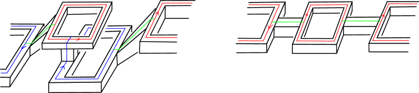
Let $A_{1},\dots,A_{2g+n}$ be oriented annuli and $B_{1},\dots,B_{g},C_{1},\dots,C_{g+n-1}$ be bands satisfying the condition $\spadesuit$ in $M$. These look like some embeddings of the union of annuli and bands as in Figure 11. Thicken these (denoted by $N$) and consider curves with colors as in Figure 15. In this figure, a part of the core curve of $A_{2i}$, which is also one edge of the band $B_{i}$ is replaced with the other three edges of $B_{i}$ for each $1\leq i\leq g$. A small neighborhood $F$ of these curves in $\partial N$ is homeomorphic to $\Sigma_{g,n+1}$ with a spine as in Figure 10. Let $K_{2i-1}$ denote the red curve coming from $A_{2i-1}$ and $K_{2i}$ the blue curve coming from $A_{2i}$ and $B_{i}$ for $1\leq i\leq g$, and $w_{j}$ the green curve coming from $C_{j}$ for $1\leq j\leq g+n-1$. For each $1\leq i\leq 2g+n$, fix an essential arc $\alpha_{i}$ in $A_{i}$ such that it is disjoint from $w_{j}$ for $1\leq j\leq g+n-1$ and $K_{l}$ for $l\neq i$, and let $D_{i}$ be an essential disk in $N$ obtained by thickening $\alpha_{i}$. Then each $\partial D_{i}$ intersects $\partial F$ twice with the opposite orientations and $D_{i}$’s cut $N$ into a ball. Therefore, $F$ gives $N$ the structure of $\Sigma_{g,n+1}\times[-1,1]$ so that $F$ is $\Sigma_{g,n+1}\times\{1\}$. The colored curves play a role of a spine of $\Sigma_{g,n+1}$. We get a surface corresponding to $\Sigma_{g,n+1}\times\{0\}$ with a spine obtained by projecting the curves along the product structure. In other word, the surface $\Sigma_{g,n+1}\times\{0\}$ with its spine is isotopic to $F$ with its spine in $M$. We can easily show that the operations in Subsections 4.1 and 4.2 are inverses of each other.

References

- [1] J. W. Alexander. A lemma on systems of knotted curves. Proceedings of the National Academy of Sciences, 9(3):93–95, 1923.
- [2] A. Conway, S. Friedl and G. Herrmann. Linking forms revisited. Pure and Applied Mathematics Quarterly, volume 12, Number 4, 493–515, 2016.
- [3] S. Garoufalidis and J. Levine. Tree-level invariants of three-manifolds, Massey products and the Johnson homomorphism. In Graphs and patterns in mathematics and theoretical physics, volume 73 of Proc. Sympos. Pure Math., pages 173–203. Amer. Math. Soc., Providence, RI, 2005.
- [4] H. Goda and T. Sakasai. Homology cylinders and sutured manifolds for homologically fibered knots. Tokyo J. Math., 36(1):85–111, 2013.
- [5] K. Habiro. Claspers and finite type invariants of links. Geom. Topol. 4 (2000), 1–83.
- [6] A. Kawauchi and S. Kojima. Algebraic classification of linking pairings on 3-manifolds. Math. Ann. 253 (1980), 29–42.
- [7] G. Massuyeau and J.-B. Meilhan. Equivalence relations for homology cylinders and the core of the Casson invariant. Trans. Amer. Math. Soc. 365 (2013), 5431–5502.
- [8] S. Matveev. Generalized surgeries of three-dimensional manifolds and representations of homology spheres. Mat. Zametki 42 (1987) 268–278, 345 (Russian); English translation: Math. Notes 42 (1987), 651–656.
- [9] R. Myers. Open book decompositions of 3manifolds. Proc. Amer. Math. Soc., 72(2):397–402, 1978.
- [10] Y. Nozaki. Every lens space contains a genus one homologically fibered knot. Illinois J. Math. volume 62, Number 1–4 (2018), 99–111.
- [11] N. Sekino. Lens spaces which are realizable as closures of homology cobordisms over planar surfaces. Illinois J. Math. volume 64, Number 4 (2020), 481–492.
- [12] Wall, C.T.C.: Quadratic forms on finite groups, and related topics, Topology 2, 281–298 (1964).
GRADUATE SCHOOL OF MATHEMATICAL SCIENCES, THE UNIVERSITY OF TOKYO, 3-8-1 KOMABA, MEGURO–KU, TOKYO, 153-8914, JAPAN
E-mail address: [email protected]