The equivalence between Stein variational gradient descent
and black-box variational inference
Abstract
We formalize an equivalence between two popular methods for Bayesian inference: Stein variational gradient descent (SVGD) and black-box variational inference (BBVI). In particular, we show that BBVI corresponds precisely to SVGD when the kernel is the neural tangent kernel. Furthermore, we interpret SVGD and BBVI as kernel gradient flows; we do this by leveraging the recent perspective that views SVGD as a gradient flow in the space of probability distributions and showing that BBVI naturally motivates a Riemannian structure on that space. We observe that kernel gradient flow also describes dynamics found in the training of generative adversarial networks (GANs). This work thereby unifies several existing techniques in variational inference and generative modeling and identifies the kernel as a fundamental object governing the behavior of these algorithms, motivating deeper analysis of its properties.
1 Introduction
The goal of Bayesian inference is to compute the posterior over a variable of interest . In principle, this posterior may be computed from the prior and the likelihood of observing data , using the equation
| (1) |
We denote the posterior as for convenience of notation. Unfortunately, the integral in the denominator is usually intractable, which motivates variational inference techniques, which approximate the true posterior with an approximate posterior , often by minimizing the KL divergence . In this paper, we consider two popular variational inference techniques, black-box variational inference (Ranganath et al., 2014) and Stein variational gradient descent (Liu & Wang, 2016), and show that they are equivalent when viewed as instances of kernel gradient flow.
2 Stein variational gradient descent
Stein variational gradient descent (Liu & Wang, 2016), or SVGD, is a technique for Bayesian inference that approximates the true posterior with a set of particles .
In the continuous-time limit of small step size, each particle undergoes the update rule
| (2) |
where denotes the empirical distribution of particles at time :
| (3) |
and is a user-specified kernel function, such as the RBF kernel .
3 Black-box variational inference
Black-box variational inference (Ranganath et al., 2014), or BBVI, is another technique for Bayesian inference that approximates the true posterior with an approximate posterior , where is a family of distributions parameterized by . In BBVI, we maximize the evidence lower bound, or ELBO, objective
| (5) |
by gradient ascent on . This procedure effectively minimizes the KL divergence between and the true posterior , since the KL divergence and the ELBO objective differ by only the evidence , which is constant w.r.t. :
| (6) |
Our claim is:
Claim 1.
To see this, we observe that the evolution of the parameters under gradient ascent is governed by
| (7) |
Next, we specialize to the case where the family of approximate posteriors is parameterized via the reparameterization trick (Kingma & Welling, 2014). That is, suppose that there exists a fixed distribution and a parameterized function such that the following two sampling methods result in the same distribution over :
| (8) |
As an example, the family of normal distributions may be reparameterized as
| (9) |
In this setting, Roeder et al. (2017) and Feng et al. (2017) noted that
| (10) | ||||
Now, we consider the dynamics of a sample under the parameter dynamics (7). By the chain rule, we have that
| (11) |
Let us introduce the neural tangent kernel of Jacot et al. (2018)
| (12) |
and define
| (13) |
making the additional assumption that is injective. Note that if , then and are both -by- matrices that depend on . Then, substituting (7) and (10) into (11), we find that the samples satisfy
| (14) | ||||
| (15) | ||||
| (16) |
Comparing (16) with the SVGD dynamics (4), we find an exact correspondence between SVGD and BBVI, where in BBVI, the kernel is given by (13) and defined by the neural tangent kernel.
3.1 Example: a Gaussian variational family
As an example, consider the family of multivariate normal distributions , parameterized by an invertible matrix and a vector , with the relation . This variational family is reparameterizable with
| (17) |
In this setting, the kernel (13) becomes
| (18) |
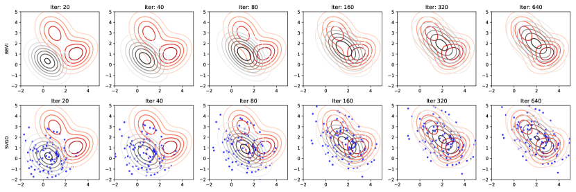
where is the identity matrix. In the continuous-time and many-particle limit, BBVI with the parameterization (17) produces the same sequence of approximate posteriors as SVGD with the kernel (18). Figure 1 compares the sequence of approximate posteriors generated by BBVI and SVGD with the theoretically equivalent kernel (18) in fitting a bimodal 2D distribution; we see that the agreement is quite close.
It is instructive to perform the computation of (18) explicitly. We use index notation with Einstein summation notation, where indices that appear twice are implicitly summed over. We have that and
| (19) |
so that the neural tangent kernel is
| (20) | ||||
| (21) | ||||
| (22) |
or in vector notation. Then, using the definition (13) and substituting and , we arrive at (18).
4 Motivating a Riemannian structure
In the previous section, we found that SVGD and BBVI both correspond to particle dynamics of the form
| (23) |
One peculiar feature of the BBVI dynamics is that the kernel depends on the current parameter , rather than being constant as the approximate posterior changes, as in the SVGD case.
In fact, we argue that this feature of BBVI is quite natural:
Claim 2.
The requirement of BBVI that the kernel depends on the current distribution naturally motivates a Riemannian structure on the space of probability distributions.
To make this claim, let us first review Euclidean and Riemannian gradient flows. In Euclidean space, following the negative gradient of a function according to
| (24) |
can lead to a minimizer of . Analogously, on a Riemannian manifold , following the negative Riemannian gradient of a function according to
| (25) |
can lead to a minimizer of . Here, is a positive-definite matrix-valued function called the Riemannian metric, which defines the local geometry at and perturbs the Euclidean gradient pointwise. Note that in the case that is the identity matrix for all , Riemannian gradient flow reduces to the Euclidean gradient flow.
Next, we review Wasserstein gradient flows, which generalize gradient flows to the space of probability distributions (Ambrosio et al., 2008). Here, we consider the set of all probability distributions over a particular space formally as an “infinite-dimensional” manifold , and we consider a function . In variational inference, the most relevant such function is the KL divergence , where we are interested in finding an approximate posterior that minimizes . Analogous to before, a minimizer of may be obtained by following the analogue of a gradient; the trajectory of the distribution turns out to take the form of the PDE
| (26) |
Here, serves as the correct analogue of the gradient of evaluated at , and it turns out that for the variational inference case . This function is known variously as the functional derivative, first variation, or von Mises influence function.
Now, we review the recent perspective that SVGD can be interpreted as a generalized Wasserstein gradient flow under the Stein geometry (Liu, 2017; Liu et al., 2019; Duncan et al., 2019). We follow the presentation of Duncan et al. (2019) and refer to it for a rigorous treatment. To set the stage, we take a non-parametric view of the SVGD update (2), in which the dependence on is interpreted as dependence on the distribution itself:
| (27) |
Substituting and the linear operator defined by
| (28) |
we have
| (29) |
Under these dynamics, the probability distribution evolves according to the PDE
| (30) |
Comparing (30) with (26), we see that (30) defines a modified gradient flow in which the gradient is perturbed by the operator .
We now advocate for generalizing Wasserstein gradient flow in the same way that Riemannian gradient flow generalizes Euclidean gradient flow. The operator perturbs the gradient in a way analogous to how the Riemannian metric perturbs the Euclidean gradient in (25), so the operator thereby defines an analogue of a Riemannian metric on . However, there is no fundamental reason that must have the restrictive form prescribed by (28). Indeed, because is analogous to the Riemannian metric , it is natural to let the kernel, whose action defines the operator , depend on the current value of . It is also natural to allow the kernel to output a matrix rather than a scalar so that may mix all components of . Duncan et al. (2019) in fact speculate on these possibilities (Remarks 17 and 1).
With these considerations in mind, we propose replacing (28) with
| (31) |
where the kernel now depends on and outputs a matrix. This defines a gradient flow by (30) that we will refer to as kernel gradient flow.111To further the analogy between Euclidean and Riemannian gradient flow and Wasserstein and kernel gradient flow, note that just as setting the Riemannian metric to identity matrix for all reduces Riemannian to Euclidean gradient flow, setting to the identity operator for all reduces kernel to Wasserstein gradient flow. The special “Euclidean” Riemannian metric obtained this way is the central object of the Otto calculus (Otto, 2001; Ambrosio et al., 2008).
Once has the form (31), BBVI may naturally be regarded as an instance of kernel gradient flow, in which the kernel is the neural tangent kernel which depends on the current distribution . More abstractly, we see that the neural tangent kernel defines a Riemannian metric on the space of probability distributions. We summarize the perspective that this framework gives on variational inference:
Claim 3.
SVGD updates generate a kernel gradient flow of the loss function , with a Riemannian metric determined by the user-specified kernel.
Claim 4.
BBVI updates generate a kernel gradient flow of the loss function , with a Riemannian metric determined by the neural tangent kernel of .
5 Beyond variational inference: GANs as kernel gradient flow
We now argue that the kernel gradient flow perspective we have developed describes not only SVGD and BBVI, but also describes the training dynamics of generative adversarial networks (Goodfellow et al., 2014).
Generative adversarial networks, or GANs, are a technique for learning a generator distribution that mimics an empirical data distribution . The generator distribution is defined implicitly as the distribution obtained by sampling from a fixed distribution , often a standard normal, and running the sample through a neural network called the generator. The learning process is facilitated by another neural network called the discriminator that takes a sample and outputs a real number, and is trained to distinguish between a real sample from and a fake sample from . The generator and discriminator are trained simultaneously until the discriminator is unable to distinguish between real and fake samples, at which point the generator distribution hopefully mimics the data distribution .
For many GAN variants, the rule to update the generator parameters can be expressed in the continuous-time limit as
| (32) |
or by the chain rule,
| (33) |
The discriminator parameters are updated simultaneously to minimize a separate discriminator loss , but it is common for theoretical purposes to assume that the discriminator achieves optimality at every training step. Denoting this optimal discriminator as (i.e. setting for ), we have
| (34) |
This matches the BBVI update rule (10) with replaced by the discriminator . Hence, analogous to (16), the generated points satisfy
| (35) |
where here is defined as in (13) by the neural tangent kernel of the generator . Finally, it was observed that the optimal discriminator of the minimax GAN equals the functional derivative of the Jensen–Shannon divergence (Chu et al., 2019, 2020); hence we conclude:
Claim 5.
Minimax GAN updates generate a kernel gradient flow of the Jensen–Shannon divergence , with a Riemannian metric determined by the neural tangent kernel of the generator .
Similarly, non-saturating and Wasserstein GAN updates generate kernel gradient flows on the directed divergence and Wasserstein-1 distance respectively.
6 Conclusion
We have cast SVGD and BBVI, as well as the dynamics of GANs, into the same theoretical framework of kernel gradient flow, thus identifying an area ripe for further study.
References
- Ambrosio et al. (2008) Ambrosio, L., Gigli, N., and Savaré, G. Gradient flows: in metric spaces and in the space of probability measures. Springer Science & Business Media, 2008.
- Chu et al. (2019) Chu, C., Blanchet, J., and Glynn, P. Probability functional descent: A unifying perspective on GANs, variational inference, and reinforcement learning. In Proceedings of the 36th International Conference on Machine Learning, volume 97 of Proceedings of Machine Learning Research, pp. 1213–1222, 2019.
- Chu et al. (2020) Chu, C., Minami, K., and Fukumizu, K. Smoothness and stability in GANs. In International Conference on Learning Representations, 2020.
- Duncan et al. (2019) Duncan, A., Nüsken, N., and Szpruch, L. On the geometry of Stein variational gradient descent. arXiv preprint arXiv:1912.00894, 2019.
- Feng et al. (2017) Feng, Y., Wang, D., and Liu, Q. Learning to draw samples with amortized Stein variational gradient descent. In UAI, 2017.
- Goodfellow et al. (2014) Goodfellow, I., Pouget-Abadie, J., Mirza, M., Xu, B., Warde-Farley, D., Ozair, S., Courville, A., and Bengio, Y. Generative adversarial nets. In Advances in neural information processing systems, pp. 2672–2680, 2014.
- Jacot et al. (2018) Jacot, A., Gabriel, F., and Hongler, C. Neural tangent kernel: Convergence and generalization in neural networks. In Advances in neural information processing systems, pp. 8571–8580, 2018.
- Kingma & Welling (2014) Kingma, D. P. and Welling, M. Auto-encoding variational Bayes. 2014.
- Liu et al. (2019) Liu, C., Zhuo, J., Cheng, P., Zhang, R., and Zhu, J. Understanding and accelerating particle-based variational inference. In Proceedings of the 36th International Conference on Machine Learning, volume 97 of Proceedings of Machine Learning Research, pp. 4082–4092, 2019.
- Liu (2017) Liu, Q. Stein variational gradient descent as gradient flow. In Advances in Neural Information Processing Systems, pp. 3115–3123, 2017.
- Liu & Wang (2016) Liu, Q. and Wang, D. Stein variational gradient descent: A general purpose Bayesian inference algorithm. In Advances in neural information processing systems, pp. 2378–2386, 2016.
- Lu et al. (2019) Lu, J., Lu, Y., and Nolen, J. Scaling limit of the Stein variational gradient descent: The mean field regime. SIAM Journal on Mathematical Analysis, 51(2):648–671, 2019.
- Otto (2001) Otto, F. The geometry of dissipative evolution equations: the porous medium equation. 2001.
- Ranganath et al. (2014) Ranganath, R., Gerrish, S., and Blei, D. Black box variational inference. In Proceedings of the Seventeenth International Conference on Artificial Intelligence and Statistics, pp. 814–822, 2014.
- Roeder et al. (2017) Roeder, G., Wu, Y., and Duvenaud, D. K. Sticking the landing: Simple, lower-variance gradient estimators for variational inference. In Advances in Neural Information Processing Systems, pp. 6925–6934, 2017.