The efficiency of electron acceleration by ICME-driven shocks
Abstract
We present a study of the acceleration efficiency of suprathermal electrons at collisionless shock waves driven by interplanetary coronal mass ejections (ICMEs), with the data analysis from both the spacecraft observations and test-particle simulations. The observations are from the 3DP/EESA instrument onboard Wind during the 74 shock events listed in Yang et al. 2019, ApJ, and the test-particle simulations are carried out through 315 cases with different shock parameters. A total of seven energy channels ranging from 0.428 to 4.161 keV are selected. In the simulations, using a backward-in-time method, we calculate the average downstream flux in the pitch angle. On the other hand, the average downstream and upstream fluxes in the pitch angle can also be directly obtained from the 74 observational shock events. In addition, the variation of the event number ratio with downstream to upstream flux ratio above a threshold value in terms of the shock angle (the angle between the shock normal and upstream magnetic field), upstream Alfvn Mach number, and shock compression ratio is statistically obtained. It is shown from both the observations and simulations that a large shock angle, upstream Alfvn Mach number, and shock compression ratio can enhance the shock acceleration efficiency. Our results suggest that shock drift acceleration is more efficient in the electron acceleration by ICME-driven shocks, which confirms the findings of Yang et al. 2018.
1 INTRODUCTION
Electron acceleration is a vital topic in space and astrophysical plasmas. The well-known efficient accelerators are collisionless shocks which are able to accelerate electrons to high energies. It is widely accepted that diffusive shock acceleration (DSA; Axford et al., 1977; Krymsky, 1977; Bell, 1978; Blandford & Ostriker, 1978), i.e., the combination of first-order Fermi acceleration (FFA) and shock drift acceleration (SDA), remains the dominant particle acceleration mechanism at collisionless shocks. Recently many authors have studied the acceleration of electrons. Tsuneta & Naito (1998) proposed that in solar flares the formation of an oblique fast shock below the reconnection region provides the acceleration site for nonthermal electrons of 20–100 keV by first-order Fermi acceleration (FFA) mechanism. Guo & Giacalone (2012) studied electron acceleration at the flare termination shock in large-scale magnetic fluctuations and found that electrons can be accelerated to a few MeV which can qualitatively explain the observed hard X-ray emissions. Mann et al. (2001) suggested that in the solar corona, high energetic electrons of 1 MeV can be produced by shock waves if strong magnetic field fluctuations appear near the shock transition so that electrons are allowed to cross the shock front many times by field-line meandering. Klassen et al. (2002) investigated the origin of 0.25–0.7 MeV electrons in solar energetic particle events through observations from COSTEP/SOHO and Wind 3DP instruments and concluded that the electrons measured are accelerated by coronal shock waves. Mann et al. (2006) proposed that hard X- and -rays can be generated by electrons that are accelerated by shock drift acceleration (SDA) mechanism at the termination shock during solar flares. Warmuth et al. (2009) developed a quantitative model based on radio and hard X-ray observations to study the acceleration of electrons in solar flares, and showed the possibility of shock drift acceleration at the reconnection outflow termination shock. In addition, Miteva & Mann (2007) proposed that in the solar corona energetic electrons at quasi-perpendicular shocks can be accelerated by resonant whistler wave-electron interaction. Saito & Umeda (2011) performed particle-in-cell simulations for electron acceleration at a quasi-perpendicular shock, and showed that the parallel scattering by the kinetic Alfvn turbulence, which is generated in the shock transition, suppresses the reflection of electrons during the shock drift acceleration process.
Dresing et al. (2016) determined the particle acceleration efficiency at interplanetary shock crossings observed by STEREO spacecraft, and found that only (five events) of all analyzed shocks shows a shock-associated electron intensity increase for 65–75 keV electrons. Among the five events, they found that four were associated with ICME-driven quasi-perpendicular shocks and the rest one was associated with an SIR 111stream interaction region(with an ICME embedded in) forward quasi-parallel shock. It is possible that the observed shock-associated electron intensity increase events have more occurrence frequency in quasi-perpendicular shocks than in quasi-parallel ones, although there is very poor statistics in their studies. Furthermore, Yang et al. (2018) studied the acceleration of suprathermal electrons in the energy range of 0.3–40 keV at an ICME-driven quasi-perpendicular shock with the spacecraft observations, and obtained the pitch angle enhancements and a larger downstream electron spectral index. In the statistical work of Yang et al. (2019), for those selected quasi-perpendicular and quasi-parallel shock events they found a positive correlation between the average downstream suprathermal electron flux and magnetosonic Mach number, and the downstream flux enhancement and shock compression ratio. These results implys the importance of shock drift acceleration in the acceleration of electrons at quasi-perpendicular shocks. In addition, Yang et al. (2019) concluded that there are more SEP events associated with quasi-perpendicular shocks compared to quasi-parallel shocks.
In the previous work (Kong & Qin, 2020), using test-particle simulations, we investigated the acceleration of suprathermal electrons at a quasi-perpendicular shock studied by Yang et al. (2018), suggesting the importance of shock drift acceleration in the acceleration of electrons. In this paper, using spacecraft data analysis and test particle simulations, we expand to study statistically the effect of shock parameters, such as shock angle (the angle between the shock normal and upstream magnetic field), upstream Alfvn Mach number, and shock compression ratio, on the ICME-driven shock acceleration efficiency. In addition, the theoretical models for shock acceleration efficiency are derived to compare with the observations and simulations. In Section 2, we show the observational data. We describe the numerical model in Section 3, and the models for efficient shock acceleration in Section 4. The results of observational analysis and simulations are presented in Section 5. Summary and discussion are given in Section 6.
2 Observational DATA
In the survey of Yang et al. (2018), 74 ICME-driven shocks are observed by Wind over the period from 1995 to 2004. The electron electrostatic analyzer (EESA) in the 3DP instrument (Lin et al., 1995) onboard Wind provides three-dimensional (3D) data for eight pitch angle channels in the energy range of 3 eV to 30 keV. For the shock events, the flux data of energetic electrons in the upstream and downstream of the shock (i.e., before and after the shock arrival) can be obtained from the Wind/3DP/EESA instrument.
We choose the shock event on 2000 Feb 11 observed by Wind as an example. The upstream energy spectra in all pitch angle directions averaged in a period of 10 minutes (23:14 UT–23:24 UT) prior to the shock are plotted in Figure 1, multiplied by , , , , , , , and for the pitch angles of , , , , , , , and , respectively. These spectra are assumed to be used as the initial upstream electron distribution before the shock acceleration in the simulations. In this work, we focus on the observations of the electron energy channels at 0.428, 0.634, 0.920, 1.339, 1.952, 2.849, and 4.161 keV indicated by with , 2, 3, …, 7, as listed in Table 1, from the Wind/3DP/EESA measurement. Using the data observed by Magnetic Field Investigation (MFI) (Farrell et al., 1995; Kepko et al., 1996) and Solar Wind Experiment (SWE) (Ogilvie et al., 1995) instruments onboard Wind we obtain the upstream average magnetic field nT and proton number density . Thus, the upstream Alfvn speed is with the formula , where is space permeability and is proton mass.
3 numerical model
We study the acceleration of electrons at a plane shock by using spacecraft data analysis and test-particle simulations similar to our previous work (Kong et al., 2017, 2019). Under the given shock parameters, the trajectories of test particles are traced by calculating the motion of equation of particles in the electromagnetic field
| (1) |
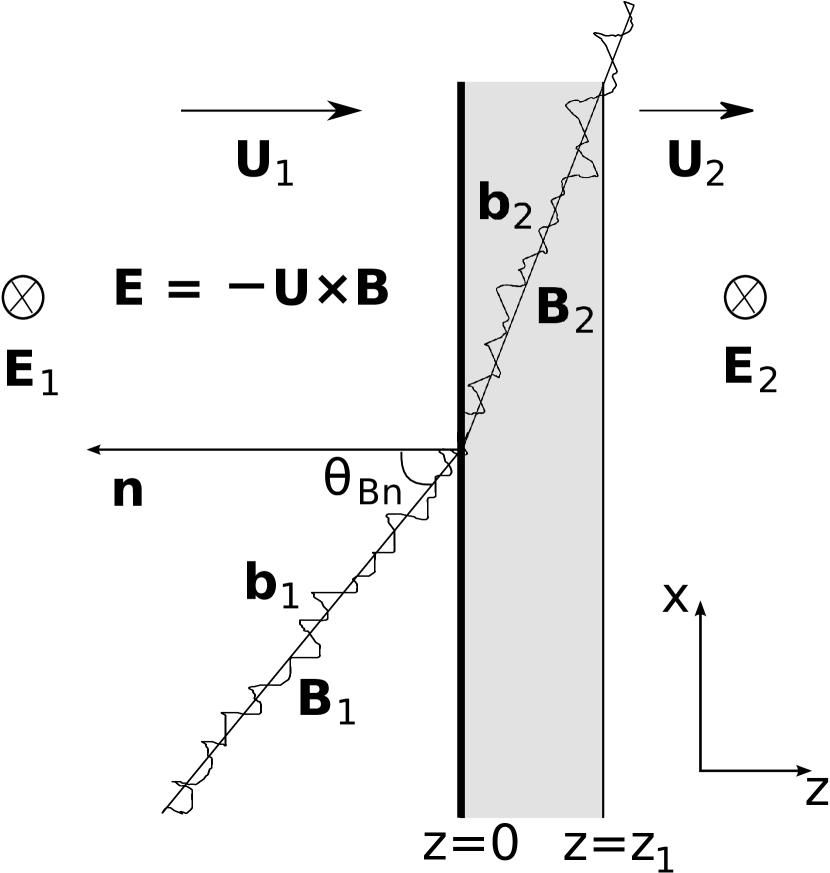
where is the particle momentum, is the electron charge, is the particle velocity, and t is time. The electric field is the convection electric field . The shock is located at , and the plasma flows from the upstream region with a speed to downstream region with a speed in the shock reference frame, as shown in Figure 2 (similar to Figure 1 in Kong & Qin (2020)). Here, the upstream speed and downstream speed can be determined by
| (2) |
and
| (3) |
with the upstream Alfvn Mach number and shock compression ratio . It will be later shown that the downstream fluxes from observations and simulations are measured in the range of from 0 to au. We assume the plasma speed in the shock transition is in the form (e.g., Qin et al., 2018)
| (4) |
where is the shock thickness and assumed to be au in this work. It is noted that is too small to be shown in Figure 2. The magnetic field, , is given by
| (5) |
where is a background magnetic field assumed to lie in – plane, and is a turbulent field perpendicular to the background field. Note that the magnetic field is taken to be a static magnetic field without the flow-advected effect for simplicity considering the high speed of particles (e.g., Fraschetti & Giacalone, 2015). The turbulent field, composed of a slab and two-dimensional (2D) components (Matthaeus et al., 1990; Mace et al., 2000; Qin et al., 2002a, b), is given by
| (6) |
where -axis in the Cartesian coordinate () system, which is used to generate the slab and 2D turbulence, is parallel to the background magnetic field .
In all simulations, the slab turbulence has a correlation length of au. The ratio of slab to 2D correlation length is 2.6 according to previous studies (Osman & Horbury, 2007; Weygand et al., 2009, 2011; Dosch et al., 2013). We define the turbulence in a periodic box of size [10,10] for the 2D component turbulence and size 25 for the slab component turbulence. A dissipation range in which low-energy electrons resonate for the slab turbulence is required, and the break wavenumber is fixed at from the slab inertial to dissipation ranges. The spectral indices of the inertial and dissipation ranges are and , respectively. Note that the pitch angle scattering corresponds to the parallel diffusion, and the resonance between particles and turbulence is not affected by the 2D turbulence assuming weak nonlinear effects. Hence, the dissipation range of 2D turbulence is ignored. We take the turbulence level, , of 0.25 in the upstream and 0.36 in the downstream of the shock. Note that the turbulent magnetic fluctuations is supposed to be perpendicular to the background magnetic field and have a zero-average in both upstream and downstream. We assume that the enhancement of the turbulence level, , from upstream to downstream, is caused by the strong disturbance of the shock wave. The detail of the varying turbulence level throughout the shock structure is very complicated. If the upstream turbulence level is set, the value of downstream turbulence level has to be obtained with theoretical modeling depending on values of different parameters, e.g., the density compression. However, for the simplicity, we use a fixed turbulence level in this work to study the acceleration efficiency of electrons by the interplanetary shock. In addition, the energy density ratio of the slab to 2D components is assumed to .
In the simulations of shock acceleration of energetic electrons, we use a method of backward tracing electron trajectories (i.e., backward-in-time method, Kong et al., 2017; Kong & Qin, 2020). For each simulation case, we want to obtain the downstream distribution of accelerated electrons under a given initial distribution (e.g., upstream flux taken as the initial distribution in this work). Therefore, we put a large number of test particles in the downstream and calculate the trajectories of those particles backward. After a period of time, the particles move back to the upstream at the initial time . The downstream distribution would be obtained with Equation 5 in Kong & Qin (2020) by calculating all the test particles. In this work each of the simulation cases does not correspond to any of the 74 shock events from the observations. It is complicated to obtain all the physical parameters for simulations in each of the observational shock events. In addition, the initial pitch angle distributions of all the observed events are difficult to be obtained; in particular, several events are even lack of observational data in some pitch angle directions. Therefore, we do not simulate the 74 observed shock events. Instead, we construct a parameter space with the shock angle , upstream Alfvn Mach number , and shock compression ratio (listed in Table 2). This allows us to obtain a total of virtual shock event cases, for each of which we perform shock acceleration simulations of electrons. Then, the acceleration efficiency of electrons at the shock with different parameters is statistically analyzed, and compared with the result from the observations.
At the end of the simulation time min, the downstream flux in the range in the pitch angle for a target energy channel is obtained based on the initial upstream distributions as shown in Figure 1, where and au. Note that the value of is set to a distance that a shock with a speed of 682 km s-1 travels within 10 min. It is also noted that the speed of 682 km s-1 happens to be equal to that of the shock on 2000 Feb 11. Actually, the exact values of and do not change the general findings in this work. More details about the backward-in-time method are given in Section 3 in Kong & Qin (2020). In order to calculate the trajectory of each test particle, we use a fourth order Runge-Kutta scheme with adaptive time stepping. Our calculation is regulated by a fifth order error estimate step with the error parameter . If we have a higher number of test particles and higher accuracy of the trajectories of test particles, we can get a more accurate downstream flux from the simulations. In our previous work (Kong & Qin, 2020), the downstream flux from the simulations are compared with the observed downstream flux. While in this work the simulated shock cases with the artificial shock parameters do not correspond to any of the observational events. Therefore, we do not directly perform comparisons of downstream flux between the simulations and observations. The input parameters for the shock and turbulence in the simulations are summarized in Table 3. The turbulence level of observations usually becomes greater near the shock surface (e.g., Kong et al., 2017), and it is not the same in different shock events. Note that the turbulence level in Table 3 is set to a fixed value upstream and downstream of the shock for a qualitative analysis. Besides, the ratio of shock thickness to the gyroradius of the electrons of minimal and maximal energy in the simulations are 30 and 10, respectively, which implies a small gyroradius of electrons compared with the shock thickness, so that the gyro-cycles of energetic electrons we study could stay in the shock transition region for a period of time.
4 Models for efficient shock acceleration
Next, we show some qualitative models for the efficient shock acceleration. Suppose that particles are accelerated by shock drift acceleration, the drift time can be written as (Kong & Qin, 2020)
| (7) |
here we assume electrons are in a completely scatter-free regime. Note that Equation (7) is strictly valid only in the shock with a perpendicular geometry. Furthermore, in order to achieve efficient acceleration, particles should not move away from the shock transition within the drift time, i.e.,
| (8) |
where the factor in the left-hand side is used to consider the average over the pitch angle of particle velocity. Note that in the left hand side of Equation (8) a change of the angle between the magnetic field and the shock normal across the shock within should be taken into account. However, we ignore the angle change for simplicity, because it is very difficult to consider this effect. Thus, for the critical value with efficient acceleration, we have
| (9) |
On the other hand, Drury (1983) showed that for each cycle of the particle crossing of the shock front the average momentum change of particles is
| (10) | |||||
The work done by electric field force is equal to the energy change, i.e.,
| (11) |
Substituting Equation (10) into Equation (11), and considering Equations (2) and (3), we get
| (12) |
For the qualitative analysis, we suppose that the particle guiding center displacement in the shock normal direction during the shock drift acceleration is only considering upstream of the shock. Then, the number of particle crossings of the shock front is
| (13) |
where is the gyro-period of particles. In order for energetic particles to be efficiently accelerated, the total energy increase is assumed to be large enough compared to the particle kinetic energy , i.e.,
| (14) |
Substituting Equation (12) into Equation (14), we obtain
| (15) |
or
| (16) |
Assuming the compression ratio is given by a representative value , from Equation (15) we have the critical value of the upstream Alfvn Mach number with efficient acceleration as
| (17) |
Similarly, assuming the upstream Alfvn Mach number is given by a representative value , from Equation (16) we have the critical value of the compression ratio with efficient acceleration as
| (18) |
Here, we obtain some qualitative models for efficient shock acceleration for critical values by assuming shock drift acceleration and quai-perpendicular shocks. It is suggested that particles are efficiently accelerated in quasi-perpendicular shocks, so these models for critical values can be used for the qualitative analysis purpose.
5 results of observational analysis and simulations
5.1 Stream of energetic particles anti-sunward
According to the previous work by Yang et al. (2018), it is noted that in some SEP events there is a stream of energetic particles in the direction away from the Sun downstream of the shock (see also, Kong & Qin, 2020). Here, we check whether this phenomenon is common. For all the 74 ICME-driven shock events from the data observed by Magnetic Field Investigation (MFI) onboard Wind we determine the magnetic field direction toward or away from the Sun by averaging the magnetic field x-component in GSE coordinates over 10 minutes before and after the shock arrival, since the GSE axis points to the Sun. Next, in terms of the pitch angle we define a modified pitch angle
| (19) |
Therefore, the electrons with a pitch angle are always sunward-streaming regardless of the sunward or anti-sunward direction of the interplanetary magnetic field. Using the data observed by the Wind/3DP/EESA measurement, we get the integrated differential intensity over the energy range of 0.428 – 4.161 keV with 10-minute average downstream of the shock for each of the modified pitch angle interval . For the 65 out of 74 ICME-driven shock events from Yang et al. (2019), we obtain , , and with the modified pitch angle nearest to , , and , respectively, and we set as the maximum of , , and . Similarly, we also get the integrated differential intensity for upstream with 10-minute average upstream of the shock. Note that 9 of the 74 shock events are excluded due to the unavailable data in some energy channels. Then, we define three parameters , , and as
| (20) |
| (21) |
and
| (22) |
Thus or when the electron beams are sunward or anti-sunward, respectively. The top, middle, and bottom panels of Figure 3 show parameters , , and , respectively, versus the shock angle for the 65 ICME-driven shock events with black circles. The red circles in the top and middle panels indicate the average and , respectively, in each shock angle interval.
In the top and middle panels of Figure 3 we can see that for most of the ICME-driven shock events there is a stream of energetic particles away from the Sun downstream of the shock. For comparison of the simulations and observations, the stream of particles in the observations has to be avoided. In order to study energetic particles accelerated by the shock not in the perpendicular direction, we need to choose the sunward particles. In the bottom panel of Figure 3, it is seen that for most observational cases the acceleration of electrons is much less efficient in the sunward direction than in the perpendicular direction. Therefore, we suggest that the strongest acceleration occurs in the perpendicular pitch-angle direction, which is consistent with the results from both the observations (Yang et al., 2018) and simulations (Kong & Qin, 2020). In this work we only consider the acceleration of electrons in the perpendicular direction for the observations and simulations.
5.2 Sample of SEPs with ICME-driven shocks from observations and simulations
In order to show the shock acceleration we select four sample observed SEP events from the 74 events with ICME-driven shocks listed in Yang et al. (2019). In Figure 4 red and black circles indicate downstream and upstream fluxes in the pitch angle, respectively, for the four observed shock events in the energy range of 0.428 – 4.161 keV, averaged over a period of 10 minutes. Each panel of the figure shows an event, with the date, shock angle, compression ratio, and Alfvn Mach number listed in the lower left corner. The figure shows that for all the observed events the flux is larger in the downstream compared with the upstream, and there is significant shock acceleration of energetic particles.
Furthermore, for each of the 315 simulation cases of the parameter combinations , we perform simulations with 10,000 test particles using the backward-in-time method, with the 10-minute averaged distribution in the pitch angle observed on 2000 Feb 11 as the initial condition and obtain the downstream flux for each of the energy channels . The results of four selected sample simulation cases are shown in Figure 5. The red circles in Figure 5 indicate the average downstream flux in the pitch angle from the simulations for the four cases in the energy range of 0.428 – 4.161 keV, and black circles show the initial distribution for simulations in the pitch angle. Similar as Figure 4, each panel of Figure 5 shows a simulation case, with the shock angle, compression ratio, and Alfvn Mach number listed in the lower left corner. It can seen that for all the four cases the simulated downstream flux is larger than the upstream flux which is used as the source for the simulations, and there is significant shock acceleration of particles in the simulations.
These sample results of observations and simulations might suggests that the shock acceleration efficiency increases with increasing shock angle from parallel to perpendicular, and also that the acceleration efficiency increases with the increase of compression ratio and Alfvn Mach number for a similar shock angle.
5.3 Shock acceleration efficiency from observations and simulations
In order to further study the shock acceleration efficiency, for the 74 observational shock events we obtain the ratio, , of downstream to upstream flux at pitch angle in each of the energy channels listed in Table 1. If the ratio is greater than a threshold value , we suppose that the shock acceleration is efficient. Here the value of is set to an arbitrary value of . Actually, we make a qualitative analysis, and the general findings do not change if is set to other values, unless or . We avoid to use a large in order to get good statistics. Furthermore, we set to study the acceleration of electrons. Therefore, we can study the effect of the shock angle , upstream Alfvn Mach number , and compression ratio on the shock acceleration efficiency from the observations. First, we divide the shock angle into different intervals, in each of which we obtain the ratio , where is the number of shock events with a high acceleration efficiency and is the total number of shock events. Similarly, we divide the upstream Alfvn Mach number and compression ratio into different intervals, and we obtain the ratio in each interval of and , respectively.
Furthermore, using the ratio, , of the downstream flux from simulations to the upstream flux we can determine that a shock with parameters could efficiently accelerate electrons if is satisfied. In this way, we can study the effect of , , and on the shock acceleration efficiency from the simulations. The various values of shock parameters, such as , , and from the observations carry different weights. However, for simplicity, we assume that the weight function is uniform. The general findings of this work, in fact, will not change under consideration of more realistic values of weight. We divide the shock angle into different intervals, in each of which we calculate the ratio . Similarly, we also divide and into different intervals to calculate the ratio in each interval of and , respectively.
Figure 6 shows the ratio versus the shock angle cosine (left panel), upstream Alfvn Mach number (middle panel), and compression ratio (right panel) in the energy channel of 0.428 keV for the observations (circles) and simulations (asterisks). Note that we use with , , and to indicate shock angle cosine , upstream Alfvn Mach number , and compression ratio , respectively. Figure 6(a) shows that for both the observations and simulations, with , i.e., quasi-perpendicular geometry, the ratio is the highest, and it decreases with the increase of the shock angle cosine . This indicates that the acceleration of electrons is more efficient at quasi-perpendicular shocks. In addition, it is shown that as , shock acceleration is very weak, i.e., the ratio . Therefore, we assume the ratio for both the observations and simulations can be fitted by a straight line
| (23) |
where is the fit parameter. Here, we fit data with . The red dashed and black solid lines in Figure 6(a) indicate the results obtained by fitting the data from the observations and simulations, respectively. The linear Pearson correlation coefficient of the y-axis values between the simulations/observations and fit line are given by /. As shown in Figure 6(a), the slope is negative, and the good correlation indicates that the linear fit can roughly exhibit the trend of with the shock angle. The fact that the value of increases with the decrease of , implies a stronger shock acceleration efficiency with increasing shock angle .
Figures 6(b) and (c) show that, if the upstream Alfvn Mach number and the compression ratio , respectively, the shock acceleration is very weak, i.e., the ratio , for both the observations and simulations. Due to the increase of ratio with increasing and , we assume that the variation of with or for both the observations and simulations can be fitted by the straight line in Equation (23) when . The red dashed and black solid lines indicate the results obtained by fitting the data from the observations and simulations, respectively. Also denoted in Figures 6(b)–(c) is the linear Pearson correlation coefficient for the simulations () and observations (). It is shown in Figures 6(b)–(c) that the slope is positive, and the fitting lines roughly exhibit the trend of with and . The increase of with and indicates a stronger shock acceleration efficiency with the increase of and .
Figures 7, 8, and 9 show plots similar to Figure 6, except in the energy channels of 0.634, 0.920, and 1.339 keV, respectively. In these figures, both the observations (circles) and simulations (asterisks) show that the ratio of event numbers with the high shock acceleration efficiency, , decreases with the shock angle cosine, and increases with the upstream Alfvn Mach number and compression ratio. For other energy channels listed in Table 1 we have similar results. It is noted that the results from observations and simulations from Figures 6, 7, 8, and 9 show quite large scatterings. The reason may be the limit of numbers and from both observations and simulations.
We assume that the shock acceleration efficiency is prominent when the shock angle is approximately or greater than the critical shock angle . The ratio can be used to show the shock acceleration efficiency. If the critical shock angle is smaller, the ratio would become larger, so that the electron shock acceleration is more efficient. In the top panel of Figure 10 we show the modeling results of the critical shock angle from Equation (9). It is seen that the critical shock angle increases with the increase of electron energy, and is very close to for the highest energy channel. The bottom panel of Figure 10 shows the negative slope, , from the linear fit of – in each energy channel as shown above for both the simulations (black asterisks) and observations (red circles). We can see that from the data of observations roughly agrees with the result from simulations. Moreover, the value of generally decreases with increasing electron energy, i.e., the shock acceleration is less efficient with the increase of electron energy. In other words, this suggests that higher energy electrons are more difficult to be accelerated by shocks.
Suppose the shock acceleration is strong when the upstream Alfvn Mach number and the compression ratio are approximately or greater than their critical values, and , respectively. The ratios and can be used to indicate the efficiency of shock acceleration. If and are smaller, and , respectively, would be greater, so that the electron shock acceleration is more efficient. In the top panels of Figures 11 and 12 we show the modeling results from Equations (17) and (18) for the critical upstream Alfvn Mach number and the critical compression ratio , respectively, with the efficient shock acceleration versus electron energy. Note that the modeling results for and depend on the characteristic parameters and , respectively. Because these modeling results are only used to qualitatively show the trends of the shock acceleration efficiency, here we arbitrarily set and . The modeling results show that and increase with the increase of electron energy. Therefore, the shock acceleration is less efficient for higher energy electrons. The bottom panels of Figures 11 and 12 show the slope, , from the linear fit of – and –, respectively, in each energy channel as shown above, for both the simulations (black asterisks) and observations (red circles). It is shown that the slope generally decreases with electron energy, i.e., the shock acceleration is less efficient with the increase of electron energy. Moreover, the slope from the data of observations is in rough agreement with the result from the simulations. From Figures 10-12 it is seen that the curves from simulations are less smooth than those from observations. The reason may be that the physical models we used have some shortcomings, and the computational resources are limited, so that our simulation results are not sufficiently accurate to fully reproduce the observations.
6 summary and discussion
We study the shock acceleration efficiency of suprathermal electrons, using spacecraft observational data for some ICME-driven shock events during 1995–2014 and test-particle simulations for cases of different shock parameters. It is suggested by Yang et al. (2018) (see also, Kong & Qin, 2020) that there exists a stream of energetic particles anti-sunward downstream of the shock in some SEP events. We check the 74 ICME-driven shock events listed in Yang et al. (2019), and find that for 65 events with complete data there is an anti-sunward beam of electrons downstream of the shock. This downstream anti-sunward beam may originate from the background solar wind rather than the shock acceleration. We need to use the sunward particles to study energetic particles accelerated by the shock along the magnetic field direction. It is shown that for most observational cases the acceleration of electrons in the sunward direction is much less efficient than in the perpendicular direction. Consequently, we suggest that the strongest acceleration occurs in the perpendicular pitch-angle direction. Therefore, in this paper the shock acceleration efficiency of electrons at pitch angle is investigated by comparing the simulations with observations.
For the 74 shock events listed in Yang et al. (2019), using data analysis on the spacecraft observations in seven energy channels ranging from 0.428 keV to 4.161 keV, we study how the efficiency of shock acceleration depends on different shock parameters, including the shock angle , upstream Alfvn Mach number , and compression ratio . In addition, we perform a similar research using data from 315 test-particle simulation cases with different shock parameters. With data from both the observations and simulations, we obtain the ratio of the average downstream to upstream flux for each shock acceleration case. Next, we get the ratio of the events with a large , i.e., (the threshold value set to here). We find that for both the observations and simulations, the ratio decreases with the increase of shock angle cosine and increases with upstream Mach number and compression ratio. This indicates that a large shock angle, Mach number, and compression ratio can contribute to enhance the shock acceleration efficiency. Furthermore, the variation of ratio with respect to the shock angle cosine , upstream Alfvn Mach number , and compression ratio is fitted by a straight line of slope through the point for the observations and simulations in different energy channels. The value of slope by fitting –, –, and –, respectively, shows that the shock acceleration is more efficient for lower energy particles compared to higher energy particles from the observations and simulations, which is obtained over a relatively small energy range. The reason for the lower acceleration efficiency in higher energy may be the following. With stronger scattering of particles by turbulence, the period of each cycle of the particle crossing of the shock front is shorter and the acceleration is more efficient (Drury, 1983; Kong et al., 2019). Furthermore, the turbulence scatters lower energy particles more easily compared to higher energy particles, so low-energy particles are accelerated easily to high energies by the shock. In addition, lower energy particles are more likely to stay in the shock transition within drift time. On the other hand, particles accelerated to higher energies may be firstly accelerated to lower energies. It is noted that if is set to some other values, the ratio probably vary, but the general findings of this paper will be the same.
We develop a model for the value of critical shock angle with high efficiency of shock acceleration, assuming shock drift acceleration of particles. We also obtain models for the critical values of upstream Mach number and compression ratio with efficient acceleration, based on the average momentum change of particles proposed by Drury (1983) for each cycle of the particle crossing of the shock front. Although there are undetermined parameters, the models may be used to qualitatively show the trend of the shock acceleration of particles. It is assumed that the shock acceleration efficiency is prominent when the shock angle, upstream Alfvn Mach number, and compression ratio are larger than their respective critical values. Consequently, if the critical values of shock angle, upstream Alfvn Mach number, and compression ratio are smaller, the electron shock acceleration is more efficient. The modeling results show that the critical values of shock angle, upstream Alfvn Mach number, and compression ratio increase with the increase of particle energy, implying stronger shock acceleration for lower energy particles. Therefore, the data of observations and simulations, as well as the theoretical modeling results, suggest that shock drift acceleration is efficient in the electron acceleration by ICME-driven shocks (Yang et al., 2018, 2019; Kong & Qin, 2020).
It should be noted that, the upper limit of slab turbulence wavenumbers in the simulations is set to m-1. It is, however, not significantly larger than the minimum resonant wavenumber (, where is the electron momentum) of low energy electrons. For example, for electrons with an energy of 0.428 and 0.634 keV, the minimum resonant wavenumber is m-1 and m-1, respectively. The break wavenumber for the slab turbulence between the inertial and dissipation ranges is . Therefore for electrons in the energy range of keV to keV the resonant wavenumber locates in the dissipation range of the slab turbulence. In addition, the upper limit of the wavenumber of 2D magnetic turbulence component is , and the dissipation range of 2D turbulence is ignored. It is considered that energetic particles are in resonance with slab turbulence in the resonant wavenumber , and parallel diffusion depends on the slab component with the assumption of quasi-linear theory, so the upper limit of the wavenumber of slab component of the magnetic turbulence is very important. We also consider that perpendicular diffusion depends on both the 2D and slab turbulence by the non-linear effects. It is more difficult to construct a 2D component turbulence with a very large wavenumber range. In addition, lower wavenumber range of 2D component can influence the perpendicular diffusion because of the non-linear effects. Therefore, we set a 2D component with a low upper limit of wavenumber.
As a result, in our simulations lower energy electrons have a narrow resonant range in the power spectrum of the turbulence compared to the observations. The simulations of the acceleration of high energy electrons, which have a large velocity, require more computational resources in order to ensure numerical accuracy. Therefore, we expect to use more powerful computational resources to increase the upper limit of the slab turbulence and the computing accuracy in the simulations in future works.
References
- Axford et al. (1977) Axford, W. I., Leer, E., & Skadron, G. 1977, Proc. ICRC (Plovdiv), 11, 132 0
- Bell (1978) Bell, A. R. 1978, MNRAS, 182, 147
- Bieber et al. (1996) Bieber, J. W., Wanner, W., & Matthaeus, W. H. 1996, J. Geophys. Res., 101, 2511
- Blandford & Ostriker (1978) Blandford, R. D., & Ostriker, J. P. 1978, ApJ, 221, L29
- Dosch et al. (2013) Dosch, A., Adhikari, L., & Zank, G. P. 2013, in 13th Int. Solar Wind Conf. (Solar Wind 13), 1539, 155
- Dresing et al. (2016) Dresing, N., Theesen, S., Klassen, A.,
- Drury (1983) Drury, L. O’C. 1983, Rep. Prog. Phys., 46, 973 & Heber, B. 2016, A&A, 588, A17
- Farrell et al. (1995) Farrell, W. M., Thompson, R. F., Lepping, R. P., & Byrnes, J. B. 1995, IEEE Trans. on Magnetics, 31, 966
- Fraschetti & Giacalone (2015) Fraschetti, F., & Giacalone, J. 2015, MNRAS, 448, 3555
- Guo & Giacalone (2012) Guo, F., & Giacalone, J. 2012, ApJ, 753, 28
- Kepko et al. (1996) Kepko, E. L., Khurana, K. K., Kivelson, M. G., et al. 1996, IEEE Transactions on Magnetics, 32, 2
- Klassen et al. (2002) Klassen, A., Bothmer, V., Mann, G., et al. 2002, A&A, 385, 1078
- Kong et al. (2017) Kong, F. J., Qin, G., & Zhang, L. H. 2017, ApJ, 845, 43
- Kong et al. (2019) Kong, F.-J., Qin, G., Wu, S.-S., Zhang, L.-H., Wang, H.-N., Chen, T., & Sun, P. 2019, ApJ, 877, 97
- Kong & Qin (2020) Kong, F. J., & Qin, G. 2020, ApJ, 896, 20
- Krymsky (1977) Krymsky, G. F. 1977, DoSSR, 234, 1306
- Lin et al. (1995) Lin, R. P., Anderson, K. A., Ashford, S., et al. 1995, Space Sci. Rev., 71, 125
- Mace et al. (2000) Mace, R. L., Matthaeus, W. H., & Bieber, J. W. 2000, ApJ, 538, 192
- Mann et al. (2006) Mann, G., Aurass, H., & Warmuth, A. 2006, A&A, 454, 969
- Mann et al. (2001) Mann, G., Classen, H. T., & Motschmann, U. 2001, J. Geophys. Res., 106, 25323
- Matthaeus et al. (1990) Matthaeus, W. H., Goldstein, M. L., & Roberts, D. A. 1990, J. Geophys. Res., 95, 20673
- Miteva & Mann (2007) Miteva, R., & Mann, G. 2007, A&A, 474, 617
- Ogilvie et al. (1995) Ogilvie, K. W., Chornay, D. J., Fritzenreiter, R. J., et al. 1995, Space Sci. Rev., 71, 55
- Osman & Horbury (2007) Osman, K. T., & Horbury, T. S. 2007, ApJ, 654, L103
- Qin et al. (2002a) Qin, G., Matthaeus, W. H., & Bieber, J. W. 2002a, Geophys. Res. Lett., 29, 1048
- Qin et al. (2002b) Qin, G., Matthaeus, W. H., & Bieber, J. W. 2002b, ApJ, 578, L117
- Qin et al. (2018) Qin, G., Kong, F. J., & Zhang, L. H. 2018, ApJ, 860, 3
- Saito & Umeda (2011) Saito, S., & Umeda, T. 2011, ApJ, 736, 35
- Tsuneta & Naito (1998) Tsuneta, S., & Naito, T. 1998, ApJ, 495, L67
- Warmuth et al. (2009) Warmuth, A., Mann, G., & Aurass, H. 2009, A&A, 494, 677
- Weygand et al. (2009) Weygand, J. M., Matthaeus, W. H., Dasso, S., et al. 2009, J. Geophys. Res., 114, A07213
- Weygand et al. (2011) Weygand, J. M., Matthaeus, W. H., Dasso, S., & Kivelson, M. G. 2011, J. Geophys. Res., 116, A08102
- Yang et al. (2018) Yang, L., Wang, L., Li, G., et al. 2018, ApJ, 853, 89
- Yang et al. (2019) Yang, L., Wang, L., Li, G., et al. 2019, ApJ, 875, 104


| 1 | 2 | 3 | 4 | 5 | 6 | 7 | |
|---|---|---|---|---|---|---|---|
| (keV) | 0.428 | 0.634 | 0.920 | 1.339 | 1.952 | 2.849 | 4.161 |
| Parameter | Values |
|---|---|
| , , , , , , , , | |
| 1.5, 2.0, 2.5, 3.0, 4.0, 5.0, 6.0 | |
| 1.5, 1.8, 2.0, 2.5, 3.0 |
| Parameter | Description | Value |
|---|---|---|
| upstream magnetic field | 7.0 nT | |
| shock thickness | 2 au | |
| upstream Alfvn speed | ||
| slab correlation length | 0.02 au | |
| 2D correlation length | ||
| two-component energy density ratio | ||
| upstream turbulence level | 0.25 | |
| downstream turbulence level | 0.36 | |
| break wavenumber of slab turbulence | 10-6 m-1 | |
| inertial spectral index | 5/3 | |
| dissipation spectral index | 2.7 |