The Effect of the Slit Configuration on the H2 1-0 S(1) to Br Line Ratio of Spatially Resolved Planetary Nebulae
Abstract
The H2 1-0 S(1)/Br ratio ((Br)) is used in many studies of the molecular content in planetary nebulae (PNe). As these lines are produced in different regions, the slit configuration used in spectroscopic observations may have an important effect on their ratio. In this work, observations and numerical simulations are used to demonstrate and quantify such effect in PNe. The study aims to assist the interpretation of observations and their comparison to models. The analysis shows that observed (Br) ratios reach only values up to 0.3 when the slit encompasses the entire nebula. Values higher than that are only obtained when the slit covers a limited region around the H2 peak emission and the Br emission is then minimised. The numerical simulations presented show that, when the effect of the slit configuration is taken into account, photoionization models can reproduce the whole range of observed (Br) in PNe, as well as the behaviour described above. The argument that shocks are needed to explain the higher values of (Br) is thus not valid. Therefore, this ratio is not a good indicator of the H2 excitation mechanism as suggested in the literature.
keywords:
planetary nebulae: general – circumstellar matter – astrochemistry – ISM: molecules – photodissociation region (PDR)1 Introduction
As the most abundant molecular species in planetary nebulae (PNe), the emission of H2 is of great interest. Molecular hydrogen lines have been detected in the near infrared (IR) spectrum of more than 130 planetary nebulae (PNe) (e.g., Treffers et al., 1976; Isaacman, 1984; Kastner et al., 1996; Lumsden et al., 2001; Guerrero et al., 2000; Davis et al., 2003; Likkel et al., 2006; Ramos-Larios et al., 2017; Gledhill et al., 2018, see also Appendix A). Kastner et al. (1996) found a H2 detection rate of 40 per cent. Recent deep imaging detections of H2 in small structures in PNe indicate that this rate may be even higher (Fang et al., 2018; Akras et al., 2017, 2020a).
Most of the published H2 spectroscopic observations of PNe uses narrow slits or small apertures111To simplify the text, only slit observations will be mentioned, but most of the discussion also applies or can be easily extended to observations with different shape apertures. including only part of the planetary nebula (see Table 2). Sometimes only extractions of the slit observation are considered. Often the authors focus on specific positions in the nebula, for example, obtaining a spectrum with a slit centred at the H2 1-0 S(1) line emission peak.
The position and width of the slit aperture during a observation have a great impact on the measured line fluxes and derived line ratios demonstrated by Fernandes et al. (2005), Gesicki et al. (2016), and Akras et al. (2020b) studies for optical atomic lines. Fernandes et al. (2005), for example, studied the effects of the nebular area covered by the slit on the atomic line ratios and derived quantities in H II regions. Their results showed that ratios of low to high-ionization lines are sensitive to this area. The ratios of [O II], [N II] and [S II] optical lines to H can be affected by up to 30% in relation to the ratio of the entire ionized nebula. The difference of the emitting regions of each of the lines (low-ionization lines are emitted in the outer layers of the nebula) is responsible for such high percentage. The effect of the slit configuration on atomic line ratios can be important when studying diagnostic diagrams or comparing observations to models as showed by Akras et al. (2020b).
It is therefore expected that the effect of the slit aperture and position can also be important for the H2 line ratios to Br as they are not produced in the same region. The H2 1-0 S(1)/Br ratio (hereafter (Br)) has been used in several studies of the molecular content of PNe, as proxies of the H2 quantity (Aleman & Gruenwald, 2004, 2011) and assisting the diagnostic of the acting excitation mechanisms (Marquez-Lugo et al., 2015).
This paper studies the effect of the slit configuration on the (Br) ratio, using observations available in the literature and numerical simulations to verify and quantify such effect. The observations used here are described in Sect. 2 and a table is given in Appendix A. The numerical simulations are described in Sect. 3. The results of the analysis of the slit configuration effect is presented in Section 4. Conclusions are summarised in Sect. 5.
2 Observations
For the present work, H2 and Br line fluxes and ratios from observations were compiled from the literature. The data collected is presented in Table 2 (see Appendix A). The table shows the (Br) line ratios obtained from spectroscopic observations of PNe and information on the corresponding slit configuration. The table also includes a few other relevant characteristics of the PNe, which are used in the present analysis.
The slit centred at the nebular centre and positioned across the entire nebula (indicated as “centred” in Fig. 1) is the most typical PN observation configuration used for optical nebular analysis, i.e., for works focused on the ionized region. Although also used in studies of the H2 component in extended objects, other common position in this case is the narrow slit positioned at the H2 emission peak (indicated as “H2 peak” in Fig 1). Observing the whole nebula is only possible for more compact and/or distant PNe. In Table 1, the observations are classified within four general slit configurations as follows:
-
•
Centred: the slit is positioned across the whole nebula passing by its centre;
-
•
H2 peak: centred at the H2 1-0 S(1) emission peak;
-
•
Whole nebula: when the slit encompass the entire nebula;
-
•
Other: all other configurations that do not falls under the previous categories or the configuration is not clear from the paper description.
This nomenclature will be used hereafter to indicate the slit positions for both observations and simulations.
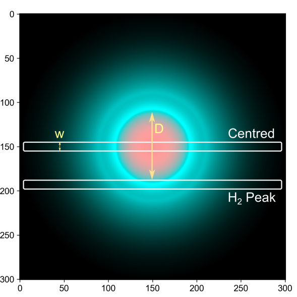
In Fig. 1, the illustration shows a round nebula, but the above classification is extended for all PNe morphologies. Bipolar PNe observations considered as centred are those with the slit across the equatorial region, perpendicular to the symmetry axis. In bipolar PNe, the waist region is usually a bright structure in H2 emission (Kastner et al., 1996). This region shows a torus or barrel-like structure. For the purposes of this paper, what is of importance is the hydrogen species that are sampled by the slit (this will become clear further in the text.). It is then not difficult to see that using the slit across this torus/barrel is analogous to the centred position for elliptical PNe, despite the angle the bipolar is observed. For bipolar PNe, observations considered as H2 peak are those where the slit samples a limited region around the wall of the torus, the wall of the lobes, or any known H2 bright position.
3 Simulations
To simulate the slit observations of the nebula, we use the Python222http://www.python.org library PyCloudy (version 0.9.6; Morisset, 2013). PyCloudy provides pseudo-3D simulations from cloudy one-dimensional models outputs. The library produces simulated line emission maps, which allow the simulation of slit observations in any configuration and the calculation of the corresponding line fluxes.
Numerical calculations of the H2 and Br emissivity in PNe were obtained with the photoionization code Cloudy (version 17.01; Ferland et al., 2017). Cloudy can simulate a photoionized nebula from the ionized to the neutral regions (photodissociation region, PDR) self-consistently. As shown in Aleman & Gruenwald (2004, 2011) and Aleman et al. (2011), this is very important for the calculation of the H2 infrared emission, in special for the PNe with high-temperature central stars.
In the present models, the ionizing source emits as a blackbody, here described by its effective temperature () and bolometric luminosity (). The gas is assumed to be spherically distributed. Models were calculated for two gas density () distributions: (i) uniform density and (ii) diffuse gas with a denser surrounding shell. For the first case, we studied density values from 103 to 105 cm-3. In the second case, the diffuse gas is assumed to have 103 cm-3 and the shell 105 cm-3. Shell models were simulated with different central star temperatures and shell distances from the central star. For each set of central star parameters, simulations with four different shell distances were studied. The position were set where H0/H = 10-4, 10-3, 10-2, and 510-1. All simulations are done with solar abundance (Grevesse et al., 2010). Although different abundance sets may change the atomic line fluxes and therefore the gas cooling rates, such differences will not affect the conclusions of this paper. Dust is included in the models uniformly mixed with the gas. Aleman & Gruenwald (2004) showed that the dust composition in the regular dust model included in photoionization codes is not a significant factor for the H2 emission (due to the similarities in the general behaviour of their opacities). On the other hand, dust size and density may greatly influence the H2 emission (Aleman & Gruenwald, 2011). Here, Cloudy models with graphite dust and dust grain size distribution typical for the ISM were explored. Dust-to-gas ratios of 310-2 and 310-3 were studied (Stasińska & Szczerba, 1999). All the models were calculated assuming a 2 kpc distance, but this value has no effect on the present results, as they are based on distance-independent quantities.
For convenience, reference values are defined in Table 1. Unless stated otherwise the model parameters are the reference values listed in that table.
| Component | Parameter | Value |
|---|---|---|
| Central Star: | Temperature | 100 000 K |
| Luminosity | 3 000 | |
| Gas: | 1 000 cm-3 | |
| Abundances | Solar | |
| (Grevesse et al., 2010) | ||
| Dust: | Material | Graphite |
| Distribution | Cloudy ISM | |
| (Mathis et al., 1977) | ||
| Dust-to-Gas Ratio | 310-3 |
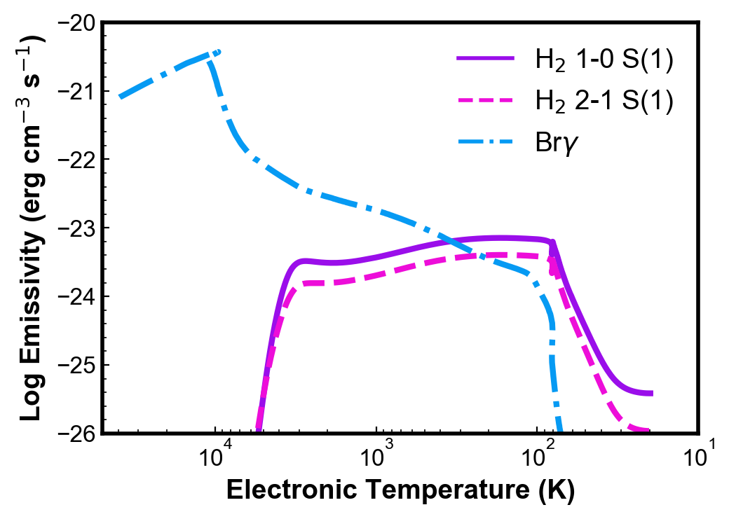
The present models simulate the physical conditions and emissivities along the PN radial outward direction from an inner radius of 1015 cm to a distance to the central star where the gas temperature decreases to 40 K. This value was chosen based on inspection of the H2 emissivity radial profiles calculated with Cloudy and to reproduce well the observations. Such stop criterion guarantee the inclusion of most of the H2 ro-vibrational lines 1-0 S(1) and 2-1 S(1) emitting region. Figure 2 provides an example of behaviour of the emissivities of such H2 lines and Br as a function of the gas temperature.
Different stopping temperatures were tested. For 100 K (cut the nebula closer to the central star), a significant portion of the total nebular H2 emission would have been ignored (unless the cloud is limited by matter). For models with 100 K, more than 70 % of the flux determined for the model with 40 K would have been ignored. For 60 K, the flux ignored is approximately 50-70 %. On the other hand, extending the nebula for very low , could produce an unrealistic large PN and the low line emissivity in such regions would not contribute much to the flux. For temperatures lower than 40 K, the H2 1-0 S(1) and 2-1 S(1) line emissivities decreases and affects very little the total calculated flux (Fig. 2). The difference in the fluxes found for 40 K and 20 K is less than a factor of two, which will not affect our conclusions.
The observation simulations were performed with PyCloudy, using a slit placed in two positions, centred and H2 peak, as discussed in the previous section. Fig. 1 shows the configurations. The two slit apertures (white boxes) are positioned over a simulated PNe (reference model). The slit length is longer than the nebula size. For both cases, we study simulations where the slit width is varied from a small fraction of the nebula diameter up to a size that includes the whole nebula. The whole nebula configuration can therefore be understood as a special limit case of both of the configurations above, when the slit width is large enough to cover the entire nebula.
4 Results
4.1 The Effect of the Slit Configuration
As the H2 1-0 S(1) and Br lines are produced in different regions in the nebula (Fig. 2) the effect of the slit configuration on the (Br) ratio in spatially-resolved observations can be significant. Indeed, Figure 3 demonstrates that both the slit configuration and the fraction of the nebula covered by the slit can have a large influence in the (Br) values.
Figure 3 shows (Br) as a function of the ratio, i.e., ratio of the slit width () to the diameter of the PN ionized region (). The ionized region diameter is used for convenience, as it is more commonly available than the total PN size (including the neutral region). When this values is not found, other diameter is used. The value will be of similar order and as this only happens for a small fraction for the sample, it will not affect the results of this work. For bipolar PNe, is assumed to be the width taken in the minor axis of the object. As H2 is more often seen in the torus/waist region or the wall of the lobes in bipolar PNe, the minor axis size would then be a better analogous dimension to of spherical PNe. The plot in Fig. 3 includes all the data collected from the literature listed in Table 2. The lower values of (Br) are limited for the observation sensitivity. This is what causes the empty lower left area in Fig. 3.
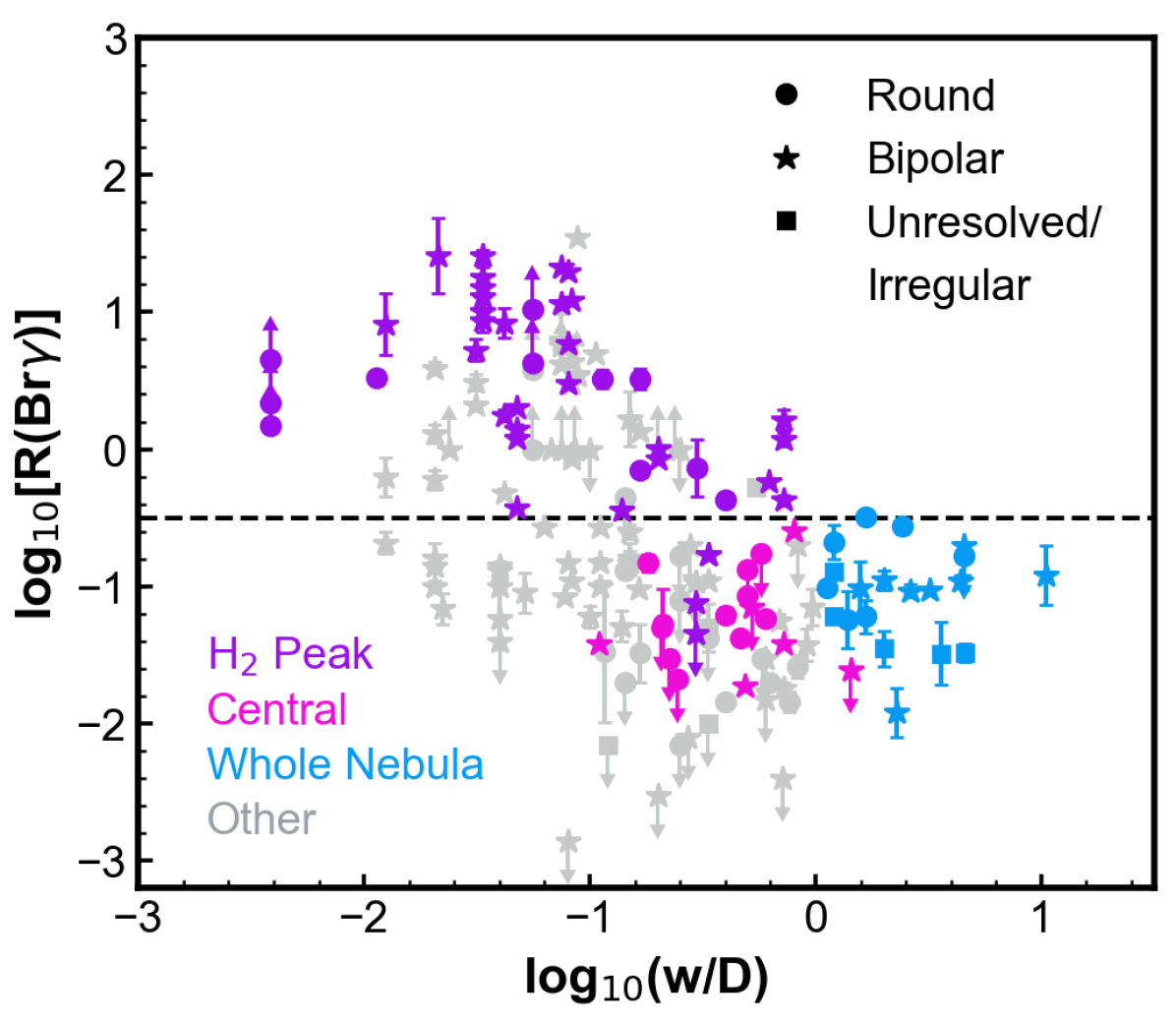
There is a clear segregation of (Br) values in Fig. 3 related to the slit configuration. The ratios obtained in the centred and whole nebula configurations show a similar range of values. In these cases, there is no indication of significant trends (Br) . The maximum value found for (Br) is 0.3 (indicated by the dashed line in the figure).
The H2 peak and other configurations exhibit the largest line ratios, which can be up to three orders of magnitude larger than the ratios measured for the whole nebula or using the centred configuration. For H2 peak, most observation are found with (Br) > 0.3.
There is also a trend for higher (Br) values being found towards small . For H2 peak observations, such trend can be naturally understood in terms of the different regions emitting H2 and Br lines and the different regions covered by the slit in each configuration. For a given nebula, is fixed, so decreasing , corresponds to using narrower slits. As decreases, the region around the H2 peak will include less Br emission, maximising the ratio (Br)(see Figs. 1 and 2). In the case of other configuration, a similar behaviour might be occurring.
For the bipolar PNe observations, a classification scheme analogue to the scheme for round objects was used. Observations considered as centred are those with the slit across the equatorial region, perpendicular to the symmetry axis. The torus is usually a bright structure in H2 emission in bipolar PNe (Kastner et al., 1996). Observations considered as H2 peak were taken with the slit sampling the wall of the torus, the wall of the lobes or at any known H2 bright position. The results found, i.e. segregation and values, are the same as found for the round PNe.
4.2 Simulations of (Br) for Different Slit Configurations
The study of models presented in this section has two goals: (i) to test our interpretation of the effect showed in the previous Section and (ii) to test if general photoionization models can reproduce the observed range of (Br) values if the slit configuration is taken into account. The second goal is of interest, as it is sometimes argued that UV excitation simulations cannot reproduce the observed values of (Br) in PNe (e.g., Marquez-Lugo et al., 2015). Comparison of observed with modelled H2 emission in PNe are done using zero- or one-dimensional models in many published works (e.g., Vicini et al., 1999; Lumsden et al., 2001; Kelly & Hrivnak, 2005; Aleman & Gruenwald, 2011; Marquez-Lugo et al., 2015; Akras et al., 2020a), but in most of them the slit configuration during the observation is not taken into account in the comparison.
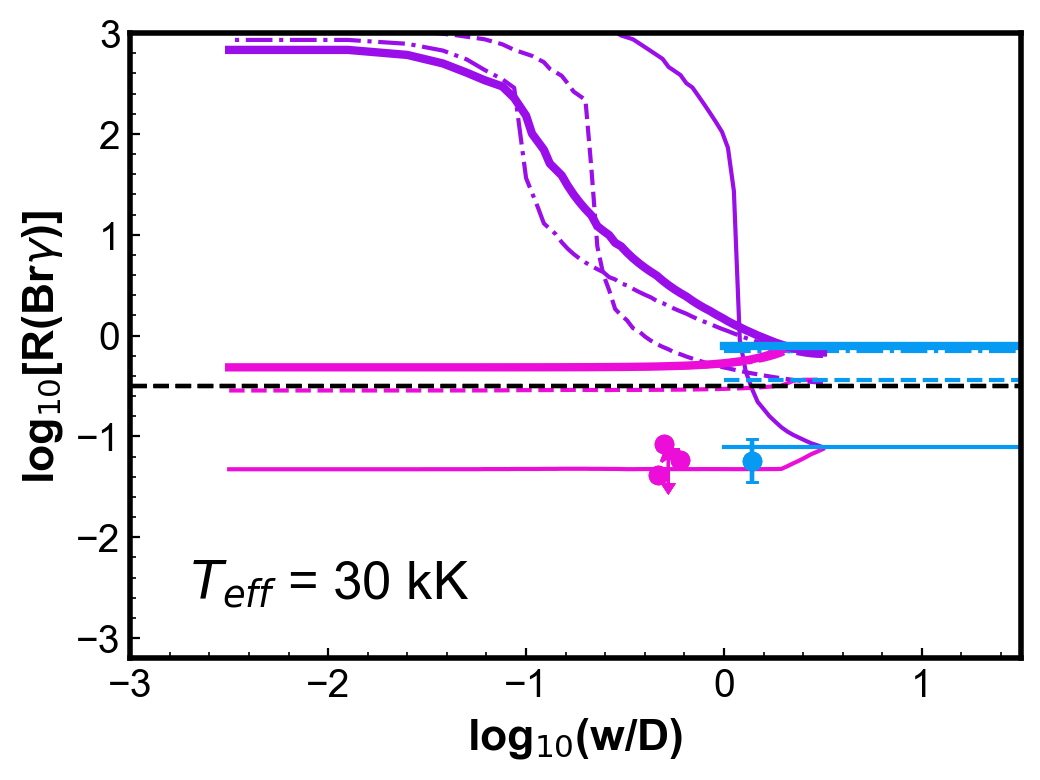
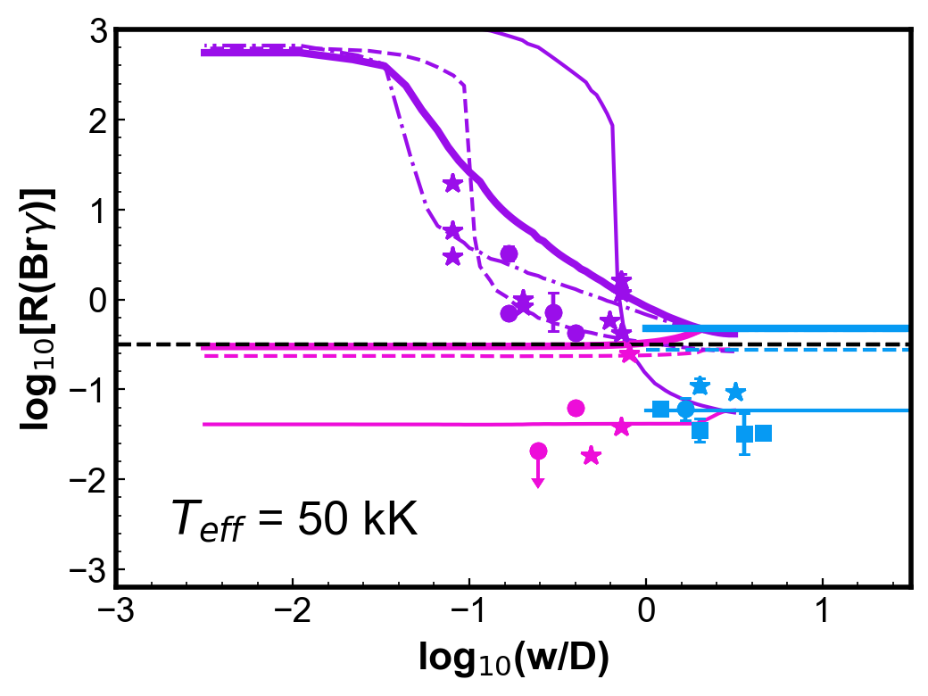
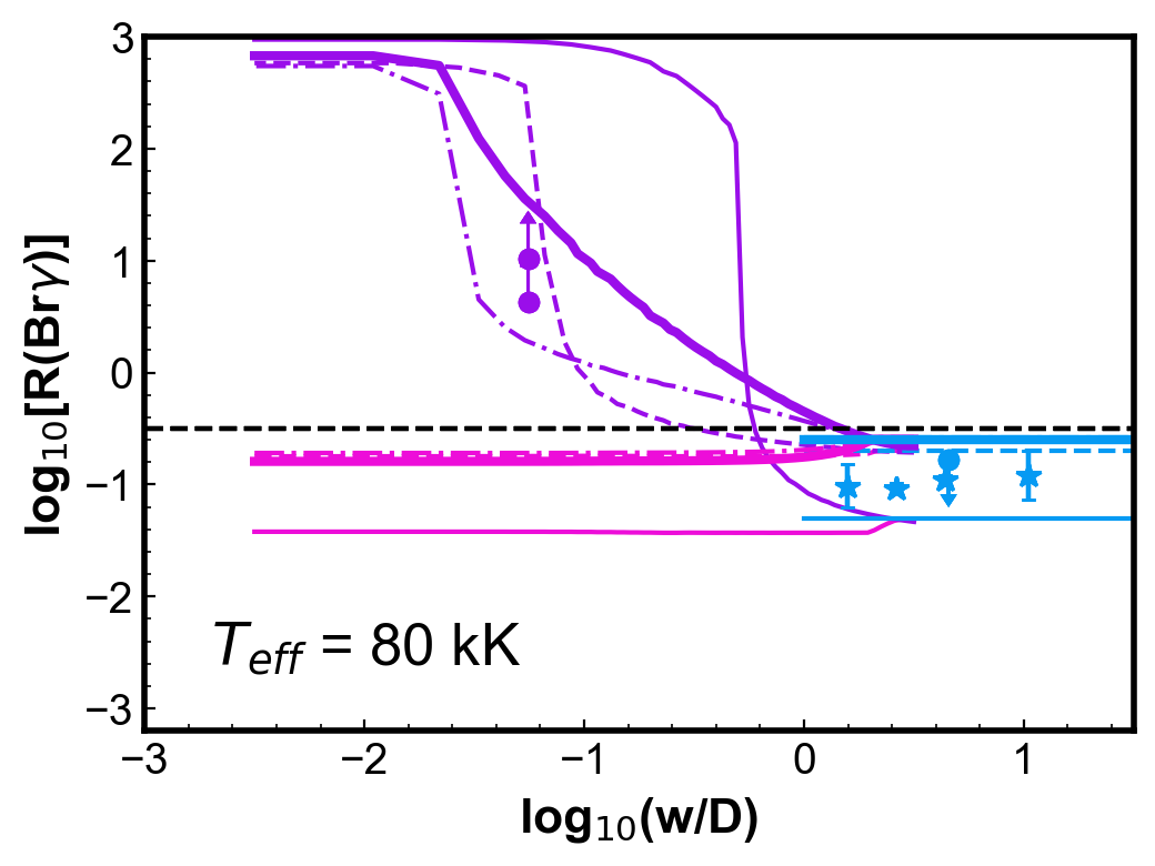
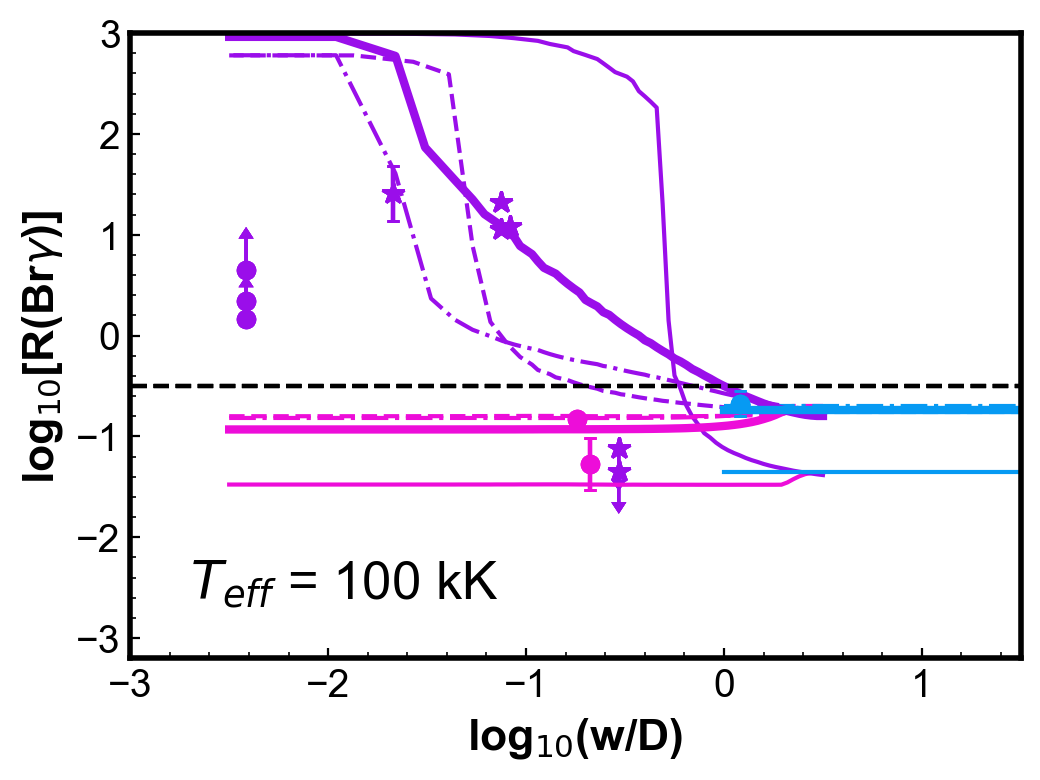
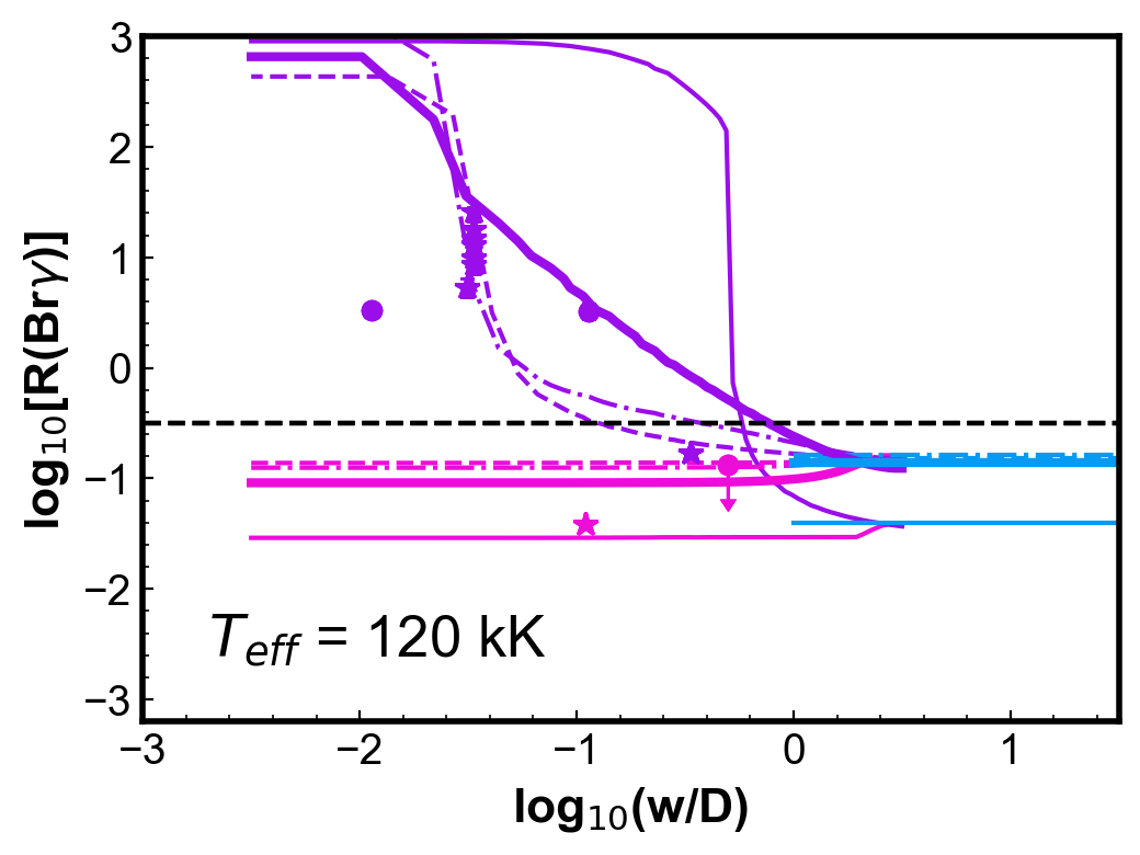
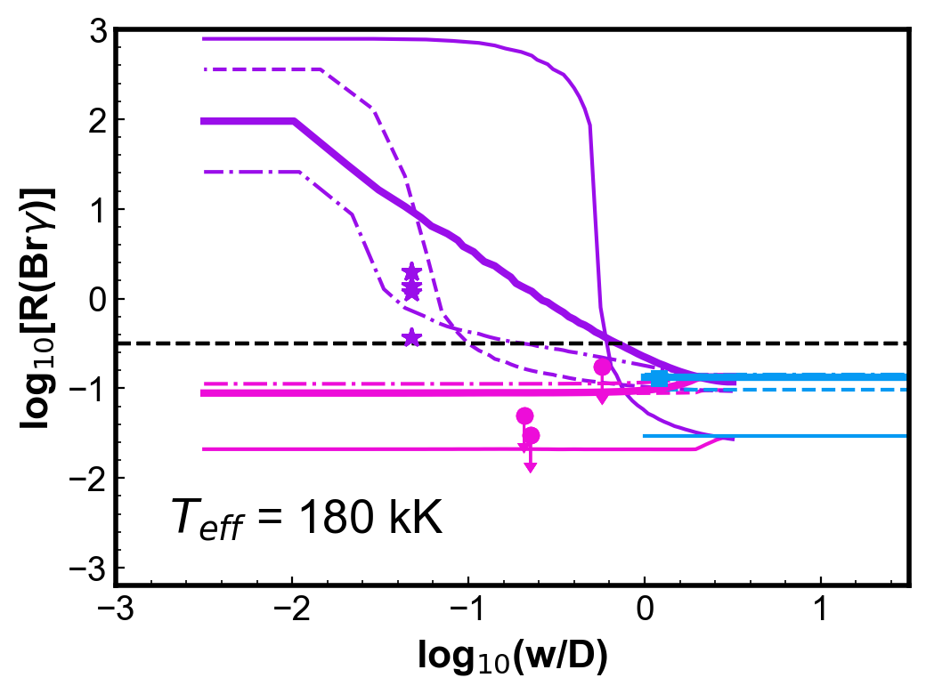
Figure 4 shows simulations of the (Br) ratio for round, uniform density PNe. Each panel shows two PN models calculated for a given and with two different dust-to-gas ratios; the other parameters are from the reference model (Table 1). For each PN model, three curves are generated: the cyan horizontal line indicates the values of (Br) calculated from fluxes integrated in the whole nebula; the pink and the purple curves show the ratios calculated using the centre and H2 peak configurations, respectively, as a function of . The colour code used for the models is thus the same as used for the observations in Fig. 3.
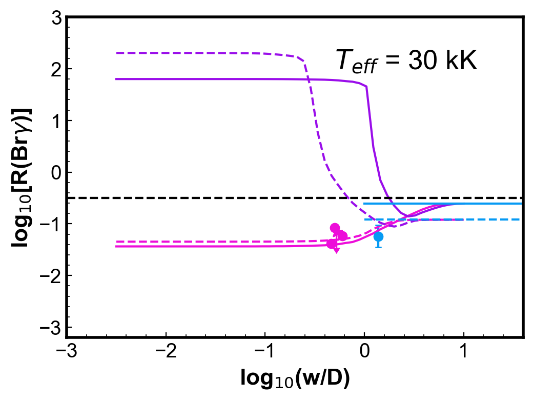
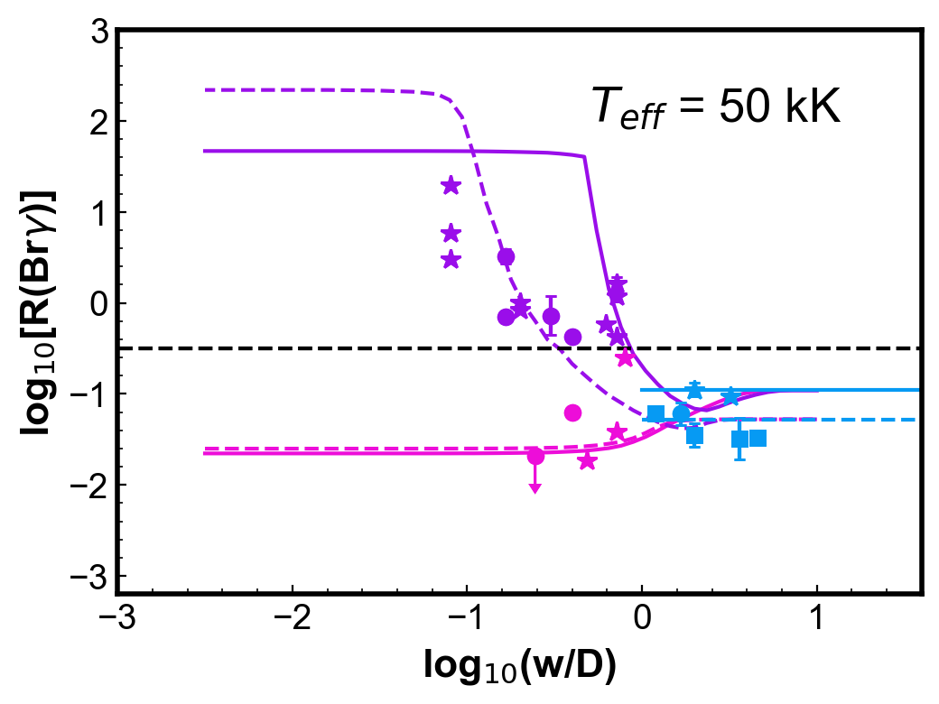
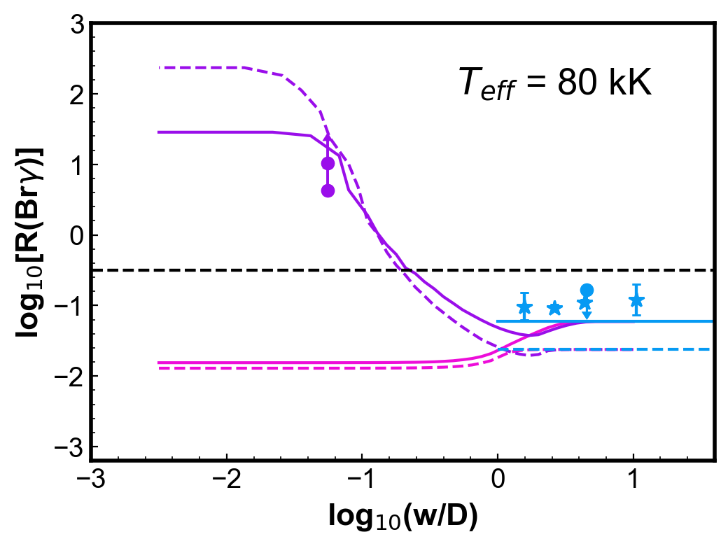
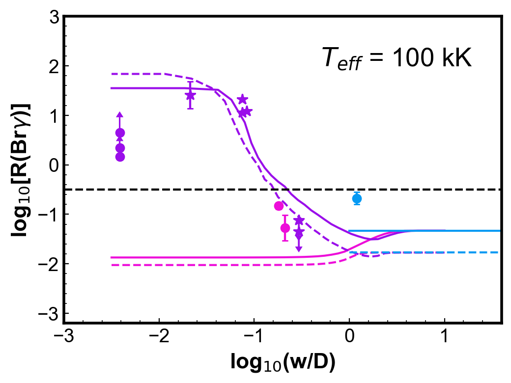
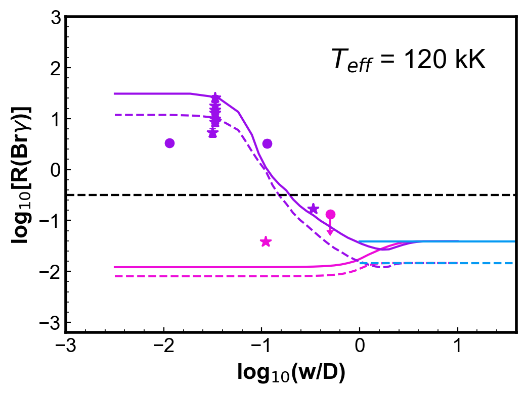
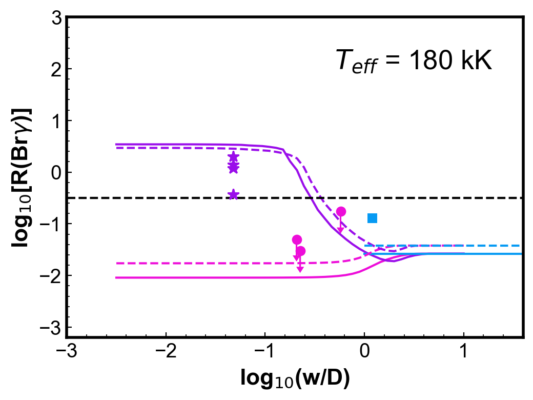
Observations of PNe with a similar temperature (within 10 kK) are included in each of the plots for comparison. Even with the simplicity of these models, the calculated values can represent reasonably well the general behaviour and, in most cases, the magnitude of the observed (Br).
For low , ratios for the centre position are smaller than for those obtained with the whole nebula configuration. The difference is less than one order of magnitude. On the other hand, for the H2 peak configuration, smaller values of produce larger values of (Br), as the slit will be covering progressively less ionized emission, without varying much the molecular emission. A plateau is reached in progressively lower for increasing . As seen in Fig 2, even in the neutral region, there is a vestigial H ionization degree. For both configurations, when gets larger than one (slit covering most to all the nebula) the values tend to the whole nebula value, as should be expected.
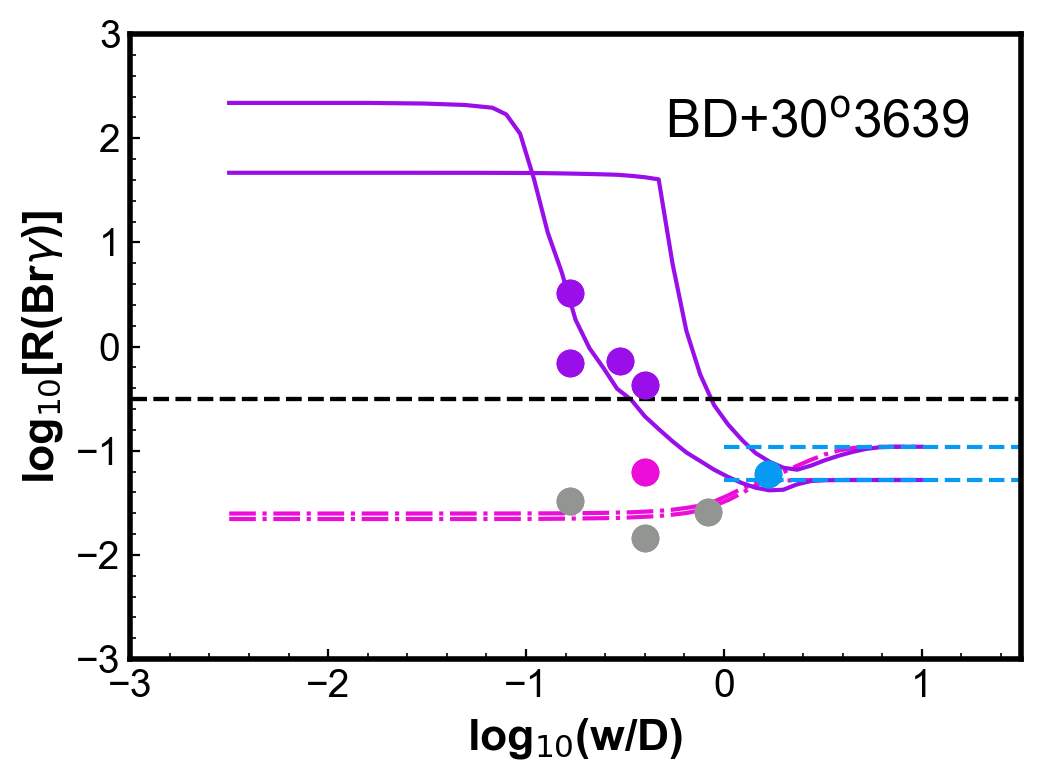
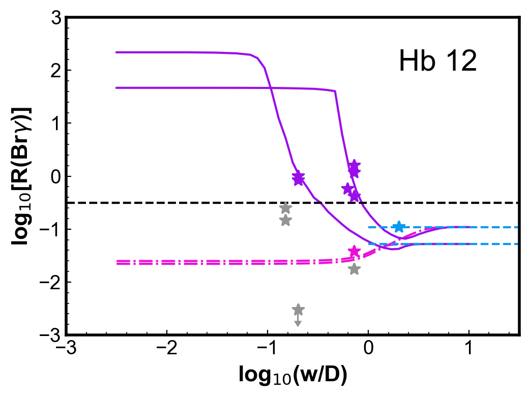
For two objects, BD+30o3639 and Hubble 12 (Hb 12), there are a number of observations with different configurations published. For these two objects, there are observations using the all the configurations we discuss previously. The observation are shown individually in the plots of Fig. 5. The models from Fig 4 with 50 kK, which is close to the object’s , are also included. The models presented in this section were not developed to fit specific objects. No attempt to match specific characteristics of the object (apart for the close ) was done. As mentioned above, these are simplified models. The goal here is only another sanity check, by verifying that the general behaviour and magnitude of the observed effect for individual objects are also reasonably reproduced by the models.
Models with different PN parameters, within typical ranges (see Aleman & Gruenwald, 2011, and references therein) were also studied. In Fig. 4, the differences in (Br) due the central star temperature and dust-to-gas ratio are shown. The general behaviour of the curves is similar for different star luminosities, within a typical PNe range. Changing the model luminosity in one order of magnitude for more or less change the curves in a similar amount as the change in dust-to-gas ratio shown. Variation in density within typical PNe values (103-105 cm-3) may account for the differences between observations and models in whole nebula and centre configurations. However, models with high densities (>105 cm-3) produces large differences between the H2 peak (Br) calculated and observed. This is natural, as dense models produce very compact nebulae, while the H2 peak observations usually probe sub-structures in more extended PNe, likely more diffuse nebulae.
Molecular hydrogen emission is often associated with dense clumpy shells or torus structures (Kastner et al., 1996; Matsuura et al., 2007; Marquez-Lugo et al., 2015; Akras et al., 2017). For this reason, simulations were also made for PNe models where a diffuse gas is surrounded by a dense shell, as describe in Sect. 3. In Fig. 6, results are shown for shells placed at different distances from the central star. Results are analogous to those from Fig. 4. They also reproduce the observations qualitatively and quantitatively. The comparison with observations shows improvement in the match of observations and models with relation to the uniform density models, especially for centre and whole nebula ratios.
Models with shell internal radius at H0/H = 10-4 (solid thin) represents well most whole nebula and centre observations. On the other hand, models with shell at H0/H = 10-3, 10-2, and 510-1, reproduces well most of the H2 peak observations, as well as some of the other configurations. This may be reflecting the ionization structures being probed by the observations. The H2 peak configuration probes structures farther form the central star, while whole nebula and centre is likely to have a stronger influence of the more ionized emission.
The simulations presented here shows that simple photoionization models can reproduce the general behaviour with and the range of observed values if they consider the slit configuration.
4.3 On (Br) as an H2 Excitation Mechanism Diagnostic
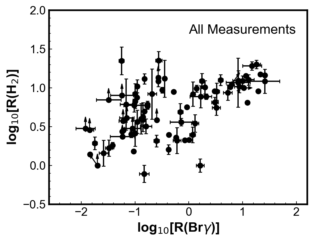
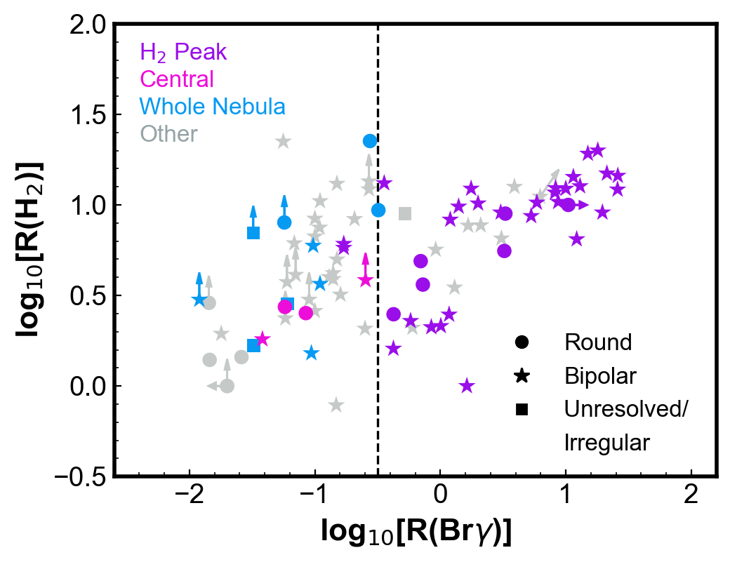
Marquez-Lugo et al. (2015) proposed the diagram (H2) vs. (Br) to analyse the excitation mechanism of H2. Figure 7 shows this diagram for the data in Table 2. In the top plot, all observations with both ratios available are shown with error bars when available. The loose positive correlation seen by Marquez-Lugo et al. (2015) is also observed here. In the plot, there is indication of two different populations, which become clear in the middle panel, where the observations are separated according to the slit configuration. The segregation in the (Br) values for different configurations seen in Fig. 3 is also seen in the diagram. Observations including the whole nebula and with the slit centred exhibit only (Br) values smaller than 0.3, as previously shown. Values (Br) > 0.3 are obtained by H2 peak observations or other configurations. For both H2 peak and whole nebula, a positive correlation between (H2) and (Br) is seen. No conclusion can be made for centre observations, as there are only a few points. All configurations show a similar range of (H2), which indicates that both H2 lines are produced in the same or very similar regions, as shown in Fig 2.
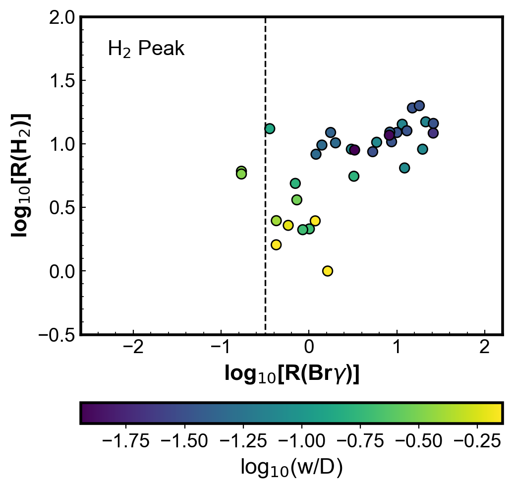
The bottom plot in Fig. 7 shows that the H2 peak points with both (H2) and (Br) high values are observed with less nebular area cover by the slit (lower ). From their diagram, Marquez-Lugo et al. (2015) conclude that shock excitation is the dominant mechanism when (H2) > 1. They based their conclusion in two arguments: (i) the thermalisation of the H2 emission of such objects (when (H2) 10) and (ii), in their words, “that shock-excitation (…) is a much more efficient excitation mechanism than UV fluorescence and thus produces higher levels of emission in the H2 lines”. However, according to the results shown here, taking into consideration the slit position in the photoionization simulations such values can easily be reached. This is not an argument against shock excitation, which cannot be discard, but the results presented here show that the observations with higher (Br) are biased by the slit effect and argument (ii) above is not valid. If photoprocesses dominate the H2 excitation, high density gas could explain the high values (H2) usually attributed to shocks. Models by Sternberg & Dalgarno (1989) showed that UV excitation (not only shocks) may thermalize the H2 level population for sufficiently high optical depths (see also discussions in Hora & Latter, 1994; Akras et al., 2020a). Marquez-Lugo et al. (2015) suggested to separate UV excitation from shocks do not necessary follows.
5 Conclusions
This paper presented the analysis of the slit configuration effect on the (Br) ratio in PNe, using observations and numerical simulations. The main results are:
-
•
The H2 1-0 S(1) and Br lines are produced in different regions in the nebula, and, therefore, the slit configuration used in the spectroscopic observations strongly affects the (Br) ratio.
-
•
For round and ring-like PNe, (Br) ratios obtained with a slit across the entire nebula passing by its centre (centred) provides similar values to those obtained by integrating the line flux over the whole nebula. Similar result is obtained for bipolar PNe when observing with the slit across the equatorial region, perpendicular to the main nebular axis (also considered here centred).
-
•
The (Br) ratios derived from observations in the centred configuration or when the whole nebula is integrated reach only values up to 0.3. Values higher than this are only obtained when the slit is positioned at the H2 peak positions.
-
•
The (Br) ratio measured with the slit at the H2 peak emission depends on the fraction of the nebula covered by the slit. The largest values of (Br) are found when the slit covers a small fraction of the nebula.
-
•
When the slit configuration is taken into account, the simple photoionization models presented here can represent very well the range of values and the general behaviour of the observed (Br).
-
•
The result above shows that the argument that shocks are needed to explain the higher values of (Br) is not valid. Therefore, this ratio is not a good indicator of the H2 excitation mechanism as suggested by Marquez-Lugo et al. (2015).
-
•
All the results showed here demonstrate the importance of considering the slit configuration in studies involving the (Br) ratio.
It is important to notice that analogous results could be obtained for shock models if they produce similar H2 and Br emission distribution. It is not the aim of this work to defend photoprocesses over shocks as the dominant H2 excitation mechanism in PNe. Here the focus is on geometrical effects and the intention is just to bring the attention to the effect of the slit configuration.
Acknowledgements
This study was financed in part by the Coordenação de Aperfeiçoamento de Pessoal de Nível Superior - Brasil (CAPES) - Finance Code 001. The author is thankful to S. Akras and H. Monteiro for useful discussions and their suggestions to improve this manuscript. This research has made use of the NASA’s Astrophysics Data System and the SIMBAD database, operated at CDS, Strasbourg, France (Wenger et al., 2000). This work has also made use of the computing facilities available at the Laboratory of Computational Astrophysics of the Universidade Federal de Itajubá (LAC-UNIFEI). The LAC-UNIFEI is maintained with grants from CAPES, CNPq and FAPEMIG.
Data Availability
The data underlying this article are available in the article. Any additional information can be request to the Author.
References
- Akras et al. (2015) Akras S., Boumis P., Meaburn J., Alikakos J., López J. A., Gonçalves D. R., 2015, MNRAS, 452, 2911
- Akras et al. (2017) Akras S., Gonçalves D. R., Ramos-Larios G., 2017, MNRAS, 465, 1289
- Akras et al. (2020a) Akras S., Gonçalves D. R., Ramos-Larios G., Aleman I., 2020a, MNRAS,
- Akras et al. (2020b) Akras S., Monteiro H., Aleman I., Farias M. A. F., May D., Pereira C. B., 2020b, MNRAS, 493, 2238
- Aleman & Gruenwald (2004) Aleman I., Gruenwald R., 2004, ApJ, 607, 865
- Aleman & Gruenwald (2011) Aleman I., Gruenwald R., 2011, A&A, 528, A74
- Aleman et al. (2011) Aleman I., Zijlstra A. A., Matsuura M., Gruenwald R., Kimura R. K., 2011, MNRAS, 416, 790
- Banerjee & Anandarao (1991) Banerjee D. P. K., Anandarao B. G., 1991, A&A, 250, 165
- Barría & Kimeswenger (2018) Barría D., Kimeswenger S., 2018, MNRAS, 480, 1626
- Bear & Soker (2017) Bear E., Soker N., 2017, ApJ, 837, L10
- Beckwith et al. (1978) Beckwith S., Persson S. E., Gatley I., 1978, ApJ, 219, L33
- Christianto & Seaquist (1998) Christianto H., Seaquist E. R., 1998, AJ, 115, 2466
- Clyne et al. (2014) Clyne N., Redman M. P., Lloyd M., Matsuura M., Singh N., Meaburn J., 2014, A&A, 569, A50
- Cuesta & Phillips (2000) Cuesta L., Phillips J. P., 2000, ApJ, 543, 754
- Davis et al. (2003) Davis C. J., Smith M. D., Stern L., Kerr T. H., Chiar J. E., 2003, MNRAS, 344, 262
- De Marco et al. (2001) De Marco O., Crowther P. A., Barlow M. J., Clayton G. C., de Koter A., 2001, MNRAS, 328, 527
- Dinerstein et al. (1988) Dinerstein H. L., Lester D. F., Carr J. S., Harvey P. M., 1988, ApJ, 327, L27
- Fang et al. (2015) Fang X., Guerrero M. A., Miranda L. F., Riera A., Velázquez P. F., Raga A. C., 2015, MNRAS, 452, 2445
- Fang et al. (2018) Fang X., Zhang Y., Kwok S., Hsia C.-H., Chau W., Ramos-Larios G., Guerrero M. A., 2018, ApJ, 859, 92
- Feibelman (1997) Feibelman W. A., 1997, ApJS, 109, 481
- Ferland et al. (2017) Ferland G. J., et al., 2017, Rev. Mex. Astron. Astrofis., 53, 385
- Fernandes et al. (2005) Fernandes I. F., Gruenwald R., Viegas S. M., 2005, MNRAS, 364, 674
- Frew (2008) Frew D. J., 2008, PhD thesis, Department of Physics, Macquarie University, NSW 2109, Australia
- García-Hernández et al. (2002) García-Hernández D. A., Manchado A., García-Lario P., Domínguez-Tagle C., Conway G. M., Prada F., 2002, A&A, 387, 955
- Geballe et al. (1991) Geballe T. R., Burton M. G., Isaacman R., 1991, MNRAS, 253, 75
- Gesicki et al. (2016) Gesicki K., Zijlstra A. A., Morisset C., 2016, A&A, 585, A69
- Gledhill et al. (2018) Gledhill T. M., Froebrich D., Campbell-White J., Jones A. M., 2018, MNRAS, 479, 3759
- Grevesse et al. (2010) Grevesse N., Asplund M., Sauval A. J., Scott P., 2010, Ap&SS, 328, 179
- Guerrero & Miranda (2012) Guerrero M. A., Miranda L. F., 2012, A&A, 539, A47
- Guerrero et al. (2000) Guerrero M. A., Villaver E., Manchado A., Garcia-Lario P., Prada F., 2000, ApJS, 127, 125
- Harrington et al. (1997) Harrington J. P., Lame N. J., White S. M., Borkowski K. J., 1997, AJ, 113, 2147
- Heap & Hintzen (1990) Heap S. R., Hintzen P., 1990, ApJ, 353, 200
- Henry et al. (1999) Henry R. B. C., Kwitter K. B., Dufour R. J., 1999, ApJ, 517, 782
- Herald & Bianchi (2004) Herald J. E., Bianchi L., 2004, ApJ, 611, 294
- Hora & Latter (1994) Hora J. L., Latter W. B., 1994, ApJ, 437, 281
- Hora et al. (1999) Hora J. L., Latter W. B., Deutsch L. K., 1999, ApJS, 124, 195
- Hsia et al. (2014) Hsia C.-H., Chau W., Zhang Y., Kwok S., 2014, ApJ, 787, 25
- Hua (1988) Hua C. T., 1988, A&A, 193, 273
- Hyung et al. (2001) Hyung S., Aller L. H., Feibelman W. A., Lee W.-B., 2001, AJ, 122, 954
- Isaacman (1984) Isaacman R., 1984, A&A, 130, 151
- Kaler & Jacoby (1989) Kaler J. B., Jacoby G. H., 1989, ApJ, 345, 871
- Kastner et al. (1996) Kastner J. H., Weintraub D. A., Gatley I., Merrill K. M., Probst R. G., 1996, ApJ, 462, 777
- Kelly & Hrivnak (2005) Kelly D. M., Hrivnak B. J., 2005, ApJ, 629, 1040
- Kwok et al. (2010) Kwok S., Chong S.-N., Hsia C.-H., Zhang Y., Koning N., 2010, ApJ, 708, 93
- Latter et al. (2000) Latter W. B., Dayal A., Bieging J. H., Meakin C., Hora J. L., Kelly D. M., Tielens A. G. G. M., 2000, ApJ, 539, 783
- Lau et al. (2016) Lau R. M., Werner M., Sahai R., Ressler M. E., 2016, ApJ, 833, 115
- Leal-Ferreira et al. (2011) Leal-Ferreira M. L., Gonçalves D. R., Monteiro H., Richards J. W., 2011, MNRAS, 411, 1395
- Likkel et al. (2006) Likkel L., Dinerstein H. L., Lester D. F., Kindt A., Bartig K., 2006, AJ, 131, 1515
- Lopez et al. (1991) Lopez J. A., Falcon L. H., Ruiz M. T., Roth M., 1991, A&A, 241, 526
- Lopez et al. (1993) Lopez J. A., Tapia M., Roth M., 1993, in Weinberger R., Acker A., eds, IAU Symposium Vol. 155, Planetary Nebulae. p. 208
- Luhman & Rieke (1996) Luhman K. L., Rieke G. H., 1996, ApJ, 461, 298
- Lumsden et al. (2001) Lumsden S. L., Puxley P. J., Hoare M. G., 2001, MNRAS, 328, 419
- Manchado et al. (2015) Manchado A., Stanghellini L., Villaver E., García-Segura G., Shaw R. A., García-Hernández D. A., 2015, ApJ, 808, 115
- Marquez-Lugo et al. (2015) Marquez-Lugo R. A., Guerrero M. A., Ramos-Larios G., Miranda L. F., 2015, MNRAS, 453, 1888
- Marston et al. (1998) Marston A. P., Bryce M., Lopez J. A., Palmer J. W., Meaburn J., 1998, A&A, 329, 683
- Mashburn et al. (2016) Mashburn A. L., Sterling N. C., Madonna S., Dinerstein H. L., Roederer I. U., Geballe T. R., 2016, ApJ, 831, L3
- Mathis et al. (1977) Mathis J. S., Rumpl W., Nordsieck K. H., 1977, ApJ, 217, 425
- Matsuura et al. (2007) Matsuura M., et al., 2007, MNRAS, 382, 1447
- Miller et al. (2019) Miller T. R., Henry R. B. C., Balick B., Kwitter K. B., Dufour R. J., Shaw R. A., Corradi R. L. M., 2019, MNRAS, 482, 278
- Miranda et al. (1997) Miranda L. F., Vazquez R., Torrelles J. M., Eiroa C., Lopez J. A., 1997, MNRAS, 288, 777
- Miranda et al. (1999) Miranda L. F., Vázquez R., Corradi R. L. M., Guerrero M. A., López J. A., Torrelles J. M., 1999, ApJ, 520, 714
- Monteiro et al. (2000) Monteiro H., Morisset C., Gruenwald R., Viegas S. M., 2000, ApJ, 537, 853
- Morisset (2013) Morisset C., 2013, pyCloudy: Tools to manage astronomical Cloudy photoionization code, Astrophysics Source Code Library (ascl:1304.020)
- O’Dell et al. (2013) O’Dell C. R., Ferland G. J., Henney W. J., Peimbert M., 2013, AJ, 145, 92
- Otsuka et al. (2013) Otsuka M., Kemper F., Hyung S., Sargent B. A., Meixner M., Tajitsu A., Yanagisawa K., 2013, ApJ, 764, 77
- Otsuka et al. (2017) Otsuka M., Parthasarathy M., Tajitsu A., Hubrig S., 2017, ApJ, 838, 71
- Phillips (2003) Phillips J. P., 2003, MNRAS, 344, 501
- Phillips et al. (1983) Phillips J. P., Reay N. K., White G. J., 1983, MNRAS, 203, 977
- Phillips et al. (1985) Phillips J. P., White G. J., Harten R., 1985, A&A, 145, 118
- Pottasch et al. (2009a) Pottasch S. R., Bernard-Salas J., Roellig T. L., 2009a, A&A, 499, 249
- Pottasch et al. (2009b) Pottasch S. R., Surendiranath R., Bernard-Salas J., Roellig T. L., 2009b, A&A, 502, 189
- Preite-Martinez et al. (1989) Preite-Martinez A., Acker A., Koeppen J., Stenholm B., 1989, A&AS, 81, 309
- Preite-Martinez et al. (1991) Preite-Martinez A., Acker A., Koeppen J., Stenholm B., 1991, A&AS, 88, 121
- Ramos-Larios et al. (2008) Ramos-Larios G., Guerrero M. A., Miranda L. F., 2008, AJ, 135, 1441
- Ramos-Larios et al. (2012) Ramos-Larios G., Vázquez R., Guerrero M. A., Olguín L., Marquez-Lugo R. A., Bravo-Alfaro H., 2012, MNRAS, 423, 3753
- Ramos-Larios et al. (2017) Ramos-Larios G., Guerrero M. A., Sabin L., Santamaría E., 2017, MNRAS, 470, 3707
- Ramsay et al. (1993) Ramsay S. K., Chrysostomou A., Geballe T. R., Brand P. W. J. L., Mountain M., 1993, MNRAS, 263, 695
- Rudy et al. (2001) Rudy R. J., Lynch D. K., Mazuk S., Puetter R. C., Dearborn D. S. P., 2001, AJ, 121, 362
- Sahai et al. (2011) Sahai R., Morris M. R., Villar G. G., 2011, AJ, 141, 134
- Shaw et al. (2006) Shaw R. A., Stanghellini L., Villaver E., Mutchler M., 2006, ApJS, 167, 201
- Shupe et al. (1995) Shupe D. L., Armus L., Matthews K., Soifer B. T., 1995, AJ, 109, 1173
- Smith et al. (1981) Smith H. A., Larson H. P., Fink U., 1981, ApJ, 244, 835
- Stanghellini et al. (2002) Stanghellini L., Villaver E., Manchado A., Guerrero M. A., 2002, ApJ, 576, 285
- Stanghellini et al. (2007) Stanghellini L., García-Lario P., García-Hernández D. A., Perea-Calderón J. V., Davies J. E., Manchado A., Villaver E., Shaw R. A., 2007, ApJ, 671, 1669
- Stanghellini et al. (2008) Stanghellini L., Shaw R. A., Villaver E., 2008, ApJ, 689, 194
- Stanghellini et al. (2016) Stanghellini L., Shaw R. A., Villaver E., 2016, ApJ, 830, 33
- Stasińska & Szczerba (1999) Stasińska G., Szczerba R., 1999, A&A, 352, 297
- Sternberg & Dalgarno (1989) Sternberg A., Dalgarno A., 1989, ApJ, 338, 197
- Storey (1984) Storey J. W. V., 1984, MNRAS, 206, 521
- Surendiranath et al. (2004) Surendiranath R., Pottasch S. R., García-Lario P., 2004, A&A, 421, 1051
- Szyszka et al. (2009) Szyszka C., Walsh J. R., Zijlstra A. A., Tsamis Y. G., 2009, ApJ, 707, L32
- Szyszka et al. (2011) Szyszka C., Zijlstra A. A., Walsh J. R., 2011, MNRAS, 416, 715
- Treffers et al. (1976) Treffers R. R., Fink U., Larson H. P., Gautier III T. N., 1976, ApJ, 209, 793
- Tylenda et al. (2003) Tylenda R., Siódmiak N., Górny S. K., Corradi R. L. M., Schwarz H. E., 2003, A&A, 405, 627
- Vázquez (2012) Vázquez R., 2012, ApJ, 751, 116
- Vicini et al. (1999) Vicini B., Natta A., Marconi A., Testi L., Hollenbach D., Draine B. T., 1999, A&A, 342, 823
- Walsh et al. (2018) Walsh J. R., et al., 2018, A&A, 620, A169
- Webster et al. (1988) Webster B. L., Payne P. W., Storey J. W. V., Dopita M. A., 1988, MNRAS, 235, 533
- Wenger et al. (2000) Wenger M., et al., 2000, A&AS, 143, 9
- Yuan et al. (2011) Yuan H. B., Liu X. W., Péquignot D., Rubin R. H., Ercolano B., Zhang Y., 2011, MNRAS, 411, 1035
Appendix A Values and references of the H2 Observations Used in the Text
Table 2 lists the H2 observations from the literature used in this paper. Column 1 shows the name of the PN and the code for the position observed according to the authors of the original paper, cited in Column 10. Column 2 and 3 gives the stellar temperature and its reference, respectively. (H2) and (Br), with errors when available, are given in Columns 4 to 7. The slit width and position used in the H2 observation are given in Columns 8 and 9, respectively. The PN morphological classification, the value assumed for its diameter, and their references are given in Column 11 to 13.
Most of the stellar temperature values are of Zanstra temperatures, with preference given for values inferred from He II lines. If effective temperatures are determined from direct star observations, preference is given for such value. If those are not available, then values determined from other methods are used.
The morphology listed in the table is a general classification based on the published literature cited in Table 2 (which is listed below). The objects with ring morphology in which a bipolar structure is not clear are considered here in the class of round nebulae. Whether such nebula is really round or torus-like (thus bipolar) will not affect the result given that the ionization structure is being taken in account during the current analysis.
| Object | (H2) | (H2) | (Br) | (Br) | Slit | H2 | Morph. | |||||
|---|---|---|---|---|---|---|---|---|---|---|---|---|
| (103 K) | Ref. | Error | Error | (arcsec) | Position | Ref. | (arcsec) | Ref. | ||||
| BD+30o3639 | 45.7 | Ph03 | 0.060 | 0.017 | 10.0 | Whole | Be78 | R | 6.0 | Ha97 | ||
| BD+30o3639 | 45.7 | Ph03 | 1.4 | 0.6 | 0.026 | 0.005 | 5.0 | Other | Ge91 | R | 6.0 | Ha97 |
| BD+30o3639 OE | 45.7 | Ph03 | 4.9 | 1.2 | 0.698 | 0.079 | 1.0 | H2 Peak | Ho99 | R | 6.0 | Ha97 |
| BD+30o3639 N Ring | 45.7 | Ph03 | 0.033 | 0.016 | 1.0 | Other | Ho99 | R | 6.0 | Ha97 | ||
| BD+30o3639 H2 Lobe | 45.7 | Ph03 | 5.6 | 1.2 | 3.238 | 0.569 | 1.0 | H2 Peak | Ho99 | R | 6.0 | Ha97 |
| BD+30o3639 Core | 45.7 | Ph03 | 1.4 | 0.015 | 2.4 | Other | Lu01 | R | 6.0 | Ha97 | ||
| BD+30o3639 Nebula | 45.7 | Ph03 | 0.062 | 2.4 | Centre | Lu01 | R | 6.0 | Ha97 | |||
| BD+30o3639 H2 Zone | 45.7 | Ph03 | 2.5 | 0.424 | 2.4 | H2 Peak | Lu01 | R | 6.0 | Ha97 | ||
| BD+30o3639 E | 45.7 | Ph03 | 3.6 | 0.4 | 0.726 | 0.351 | 1.8 | H2 Peak | Li06 | R | 6.0 | Ha97 |
| Cn 3-1 | 53.6 | Ph03 | < 0.015 | 1.8 | Other | Li06 | B | 3.0 | Mi97 | |||
| Hb 5 | 131.0 | Ph03 | < 0.200 | 5.0 | Other | We88 | B | 18.0 | Ty03 | |||
| Hb 5 up | 131.0 | Ph03 | 13.1 | 2.0 | 0.1500 | 0.010 | 2.0 | Other | Da03 | B | 18.0 | Ty03 |
| Hb 5 cen | 131.0 | Ph03 | 2.6 | 1.0 | 0.100 | 0.010 | 2.0 | Other | Da03 | B | 18.0 | Ty03 |
| Hb 5 dn | 131.0 | Ph03 | 12.2 | 2.0 | 0.270 | 0.010 | 2.0 | Other | Da03 | B | 18.0 | Ty03 |
| Hb 12 | 45.5 | Ph03 | 0.111 | 0.019 | 10.0 | Whole | Be78 | B | 5.0 | ML15 | ||
| Hb 12 | 45.5 | Ph03 | 1.0 | 0.2 | 1.629 | 0.273 | 3.6 | H2 Peak | Di88 | B | 5.0 | ML15 |
| Hb 12 | 45.5 | Ph03 | 2.3 | 0.1 | 0.579 | 0.018 | 3.1 | H2 Peak | Ra93 | B | 5.0 | ML15 |
| Hb 12 Core | 45.5 | Ph03 | < 0.003 | 1.0 | Other | HL96 | B | 5.0 | ML15 | |||
| Hb 12 3.7” E | 45.5 | Ph03 | 2.1 | 1.009 | 1.0 | H2 Peak | HL96 | B | 5.0 | ML15 | ||
| Hb 12 3.7” E 2” S | 45.5 | Ph03 | 2.1 | 0.847 | 1.0 | H2 Peak | HL96 | B | 5.0 | ML15 | ||
| Hb 12 central 1 | 45.5 | Ph03 | 1.9 | 0.4 | 0.018 | 0.002 | 3.6 | Other | LR96 | B | 5.0 | ML15 |
| Hb 12 central 2 | 45.5 | Ph03 | 1.8 | 0.2 | 0.038 | 0.002 | 3.6 | Centre | LR96 | B | 5.0 | ML15 |
| Hb 12 west | 45.5 | Ph03 | 2.5 | 0.6 | 1.175 | 0.142 | 3.6 | H2 Peak | LR96 | B | 5.0 | ML15 |
| Hb 12 east | 45.5 | Ph03 | 1.6 | 0.2 | 0.423 | 0.033 | 3.6 | H2 Peak | LR96 | B | 5.0 | ML15 |
| Hb 12 PA -5o Ring | 45.5 | Ph03 | 0.8 | 0.2 | 0.148 | 0.030 | 0.75 | Other | ML15 | B | 5.0 | ML15 |
| Hb 12 PA -5o Envelope | 45.5 | Ph03 | 2.1 | 0.4 | 0.251 | 0.028 | 0.75 | Other | ML15 | B | 5.0 | ML15 |
| He 2-111 | 196.9 | PM89 | 1.000 | 5.0 | Other | We88 | B | 74.0 | Lo93 | |||
| He 2-114 | 135.0 | KJ89 | > 1.000 | 5.0 | Other | We88 | B | 25.0 | We88 | |||
| He 3-1357 | 45.6 | Ot17 | 1.5 | 0.094 | 4.5 | Whole | GH02 | B | 1.4 | GH02 | ||
| Hf 48 Hen 2-60 | 219.4 | PM91 | > 1.000 | 5.0 | Other | We88 | B | 21.0 | We88 | |||
| Hu 1-2 | 111.0 | Ph03 | 0.039 | 1.2 | Centre | Lu01 | B | 11.0 | Fa15 | |||
| IC 418 Centre | 44.5 | Ph03 | < 0.042 | 5.0 | Other | St84 | E | 15.0 | RL12 | |||
| IC 2003 | 99.8 | Ph03 | < 0.030 | 5.0 | Other | Ge91 | R | 8.6 | Fe97 | |||
| IC 2003 Center | 99.8 | Ph03 | 0.034 | 0.040 | 1.0 | Other | Ho99 | R | 8.6 | Fe97 | ||
| IC 2003 | 99.8 | Ph03 | 0.053 | 0.031 | 1.8 | Centre | Li06 | R | 8.6 | Fe97 | ||
| IC 2165 | 190.0 | Ph03 | > 1.0 | 0.020 | 5.0 | Other | Ge91 | R | 8.0 | Mi18 | ||
| IC 2165 | 190.0 | Ph03 | < 0.030 | 1.8 | Centre | Li06 | R | 8.0 | Mi18 | |||
| IC 4406 Centre | 96.8 | Ph03 | 1.351 | 5.0 | Other | St84 | B | 30.0 | St84 | |||
| IC 4997 | 62.0 | Ph03 | < 0.200 | 10.0 | Whole | Be78 | B | 2.2 | ML15 | |||
| IC 4997 | 62.0 | Ph03 | > 3.0 | 0.012 | 0.005 | 5.0 | Whole | Ge91 | B | 2.2 | ML15 | |
| IC 5117 | 82.6 | Ph03 | 0.120 | 0.060 | 12.0 | Whole | Is84 | M | 1.1 | Hs14 | ||
| IC 5117 | 82.6 | Ph03 | 3.7 | 1.3 | 0.110 | 0.011 | 5.0 | Whole | Ge91 | M | 1.1 | Hs14 |
| IC 5117 | 82.6 | Ph03 | 0.093 | 0.009 | 3.0 | Whole | Ru01 | M | 1.1 | Hs14 | ||
| IC 5117 | 82.6 | Ph03 | 6.0 | 1.1 | 0.097 | 0.044 | 1.8 | Whole | Li06 | M | 1.1 | Hs14 |
| IC 5217 | 78.2 | Ph03 | < 0.008 | 1.8 | Other | Li06 | B | 6.6 | Hy01 | |||
| J900 | 106.0 | Ph03 | 0.210 | 0.060 | 12.0 | Whole | Is84 | R | 10.0 | Sh95 | ||
| J900 | 106.0 | Ph03 | 0.148 | 0.022 | 1.8 | Centre | Li06 | R | 10.0 | Sh95 | ||
| K 3-60 | 185.0 | Lu01 | 0.128 | 1.2 | Whole | Lu01 | I | 1.0 | St16 | |||
| K 3-67 | 59.2 | Lu01 | 0.019 | 1.2 | Centre | Lu01 | B | 2.5 | Sa11 | |||
| K 4-48 | 125.0 | Lu01 | 8.9 | 0.523 | 1.2 | Other | Lu01 | ? | 2.2 | St08 | ||
| LMC SMP-06 | 140 | Ma16 | 0.098 | 0.006 | 0.75 | Whole | Ma16 | E | 0.67 | Sh06 | ||
| LMC SMP-47 | 150 | Ma16 | 9.4 | 0.8 | 0.321 | 0.009 | 0.75 | Whole | Ma16 | E | 0.45 | Sh06 |
| LMC SMP-62 | 100 | Ma16 | > 2.9 | 0.014 | 0.002 | 0.45 | Other | Ma16 | E | 0.59 | Sh06 | |
| LMC SMP-73 | 135 | Ma16 | 22.5 | 6.1 | 0.275 | 0.037 | 0.75 | Whole | Ma16 | E | 0.31 | Sh06 |
| LMC SMP-85 | 46 | Ma16 | 1.7 | 0.4 | 0.033 | 0.005 | 0.75 | Whole | Ma16 | U | <0.163 | HB04 |
| LMC SMP-99 | 124 | Ma16 | 0.037 | 0.010 | 0.75 | Other | Ma16 | B | 0.82 | St07 | ||
| M 1-4 | 40.3 | Ph03 | < 0.02 | 1.8 | Centre | Li06 | R | 7.4 | Sa11 | |||
| M 1-6 | 34.5 | Ph03 | < 0.07 | 1.8 | Centre | Li06 | B | 3.4 | Sa11 | |||
| M 1-11 | 32.0 | Ot13 | 2.7 | 0.058 | 1.2 | Centre | Lu01 | R | 2.0 | Ot13 | ||
| M 1-11 | 32.0 | Ot13 | 2.5 | 0.2 | 0.085 | 0.006 | 1.0 | Centre | Ot13 | R | 2.0 | Ot13 |
| M 1-13 | 118.1 | PM91 | 7.7 | 2.5 | 1.667 | 0.767 | 1.8 | Other | Li06 | B | 12.0 | Li06 |
| M 1-74 | 58.0 | Ph03 | 2.8 | 0.061 | 1.2 | Whole | Lu01 | U | 1.0 | SS99 |
| Object | T | T | (H2) | (H2) | (Br) | (Br) | Slit | H2 | Morph. | |||
|---|---|---|---|---|---|---|---|---|---|---|---|---|
| (103 K) | Ref. | Error | Error | (arcsec) | Position | Ref. | (arcsec) | Ref. | ||||
| M 1-75 Lobes | 200.0 | Hu88 | 12.4 | 3.7 | 8.300 | 2.033 | 0.75 | H2 Peak | ML15 | M | 18.0 | Gu00 |
| M 1-75 Ring | 200.0 | Hu88 | 12.3 | 2.8 | 1.760 | 0.179 | 0.75 | H2 Peak | ML15 | M | 18.0 | Gu00 |
| M 1-75 Centre | 200.0 | Hu88 | 0.477 | 0.037 | 0.75 | Other | ML15 | M | 18.0 | Gu00 | ||
| M 2-9 | 43.3 | Ph03 | > 3.9 | 0.254 | 8.0 | Centre | Ph85 | B | 10.0 | HL94 | ||
| M 2-9 Core | 43.3 | Ph03 | < 0.001 | 0.8 | Other | HL94 | B | 10.0 | HL94 | |||
| M 2-9 N knot | 43.3 | Ph03 | 5.0 | 0.150 | 0.8 | Other | HL94 | B | 10.0 | HL94 | ||
| M 2-9 Lobe I | 43.3 | Ph03 | 9.1 | 3.030 | 0.8 | H2 Peak | HL94 | B | 10.0 | HL94 | ||
| M 2-9 Lobe M | 43.3 | Ph03 | 10.3 | 5.882 | 0.8 | H2 Peak | HL94 | B | 10.0 | HL94 | ||
| M 2-9 Lobe O | 43.3 | Ph03 | 9.1 | 19.61 | 0.8 | H2 Peak | HL94 | B | 10.0 | HL94 | ||
| M 4-17 PA 130o All | 127.0 | St02 | 6.5 | 1.0 | 3.070 | 0.436 | 0.75 | Other | ML15 | B | 24.0 | Gu00 |
| M 4-17 PA 40o Ring | 127.0 | St02 | 8.7 | 2.0 | 5.300 | 0.986 | 0.75 | H2 Peak | ML15 | B | 24.0 | Gu00 |
| M 4-17 PA 40o Centre | 127.0 | St02 | 7.7 | 0.6 | 2.100 | 0.123 | 0.75 | Other | ML15 | B | 24.0 | Gu00 |
| Me 2-1 | 180.0 | Ph03 | < 0.170 | 5.0 | Centre | St84 | R | 8.7 | Su04 | |||
| Me 2-1 | 180.0 | Ph03 | < 0.050 | 1.8 | Centre | Li06 | R | 8.7 | Su04 | |||
| MyCn 18 | 51.6 | Ph03 | < 0.200 | 5.0 | Other | We88 | B | 6.0 | Cl14 | |||
| Mz 1 | 139.0 | KJ89 | > 1.000 | 5.0 | Other | We88 | B | 58.4 | Ma98 | |||
| NGC 40 W Lobe | 33.8 | Ph03 | 6.1 | 4.7 | 0.069 | 0.018 | 1.0 | Other | Ho99 | B | 45.0 | LF11 |
| NGC 40 W | 33.8 | Ph03 | > 2.4 | 0.058 | 0.030 | 1.8 | Other | Li06 | B | 45.0 | LF11 | |
| NGC 40 E | 33.8 | Ph03 | < 0.040 | 1.8 | Other | Li06 | B | 45.0 | LF11 | |||
| NGC 1535 Centre | 76.3 | Ph03 | < 0.450 | 5.0 | Other | St84 | R | 35.0 | BA91 | |||
| NGC 2346 | 100.0 | Ma15 | 5.000 | 5.0 | Other | We88 | B | 47.0 | Vi99 | |||
| NGC 2346 W filament | 100.0 | Ma15 | 12.2 | 4.4 | 25.875 | 16.253 | 1.0 | H2 Peak | Ho99 | B | 47.0 | Vi99 |
| NGC 2346 W | 100.0 | Ma15 | 14.3 | 11.494 | 3.5 | H2 Peak | Vi99 | B | 47.0 | Vi99 | ||
| NGC 2346 E | 100.0 | Ma15 | 14.9 | 21.277 | 3.5 | H2 Peak | Vi99 | B | 47.0 | Vi99 | ||
| NGC 2346 S | 100.0 | Ma15 | > 11.1 | > 6.250 | 3.5 | Other | Vi99 | B | 47.0 | Vi99 | ||
| NGC 2440 | 200.0 | HH90 | 0.160 | 0.040 | 12.0 | Other | Is84 | B | 80.0 | CP00 | ||
| NGC 2440 | 200.0 | HH90 | > 13.5 | 0.270 | 0.022 | 5.0 | Other | Ge91 | B | 80.0 | CP00 | |
| NGC 2440 NE Clump | 200.0 | HH90 | 11.7 | 8.5 | 8.200 | 4.220 | 1.0 | H2 Peak | Ho99 | B | 80.0 | CP00 |
| NGC 2440 N Lobe | 200.0 | HH90 | 8.4 | 6.2 | 0.207 | 0.039 | 1.0 | Other | Ho99 | B | 80.0 | CP00 |
| NGC 2440 E Lobe | 200.0 | HH90 | 0.627 | 0.205 | 1.0 | Other | Ho99 | B | 80.0 | CP00 | ||
| NGC 2792 Centre | 114.2 | Ph03 | < 0.130 | 5.0 | Centre | St84 | R | 10.0 | Po09 | |||
| NGC 2818 20” S | 215.0 | Ph03 | > 3.420 | 5.0 | Other | St84 | B | 57.1 | Va12 | |||
| NGC 2818 30” E | 215.0 | Ph03 | > 3.540 | 5.0 | Other | St84 | B | 57.1 | Va12 | |||
| NGC 2818 | 215.0 | Ph03 | 35.000 | 5.0 | Other | We88 | B | 57.1 | Va12 | |||
| NGC 2899 | 270.0 | Fr08 | 3.000 | 5.0 | Other | We88 | B | 60.0 | Lo01 | |||
| NGC 3132 Centre | 80.1 | Ph03 | > 3.820 | 5.0 | Other | St84 | R | 90.0 | Mo00 | |||
| NGC 3132 20” N | 80.1 | Ph03 | > 4.290 | 5.0 | H2 Peak | St84 | R | 90.0 | Mo00 | |||
| NGC 3132 20” E | 80.1 | Ph03 | 10.0 | > 10.480 | 5.0 | H2 Peak | St84 | R | 90.0 | Mo00 | ||
| NGC 3132 | 80.1 | Ph03 | 10.50 | 5.0 | Other | We88 | R | 90.0 | Mo00 | |||
| NGC 3242 Centre | 89.9 | Ph03 | < 0.080 | 5.0 | Other | St84 | R | 20.0 | BK18 | |||
| NGC 3242 15” E | 89.9 | Ph03 | < 0.170 | 5.0 | Other | St84 | R | 20.0 | BK18 | |||
| NGC 3242 | 89.9 | Ph03 | < 0.007 | 5.0 | Other | Ge91 | R | 20.0 | BK18 | |||
| NGC 4071 | 118.0 | Ph03 | > 1.000 | 5.0 | Other | We88 | B | 66.7 | Be17 | |||
| NGC 5189 | 109.8 | Ph03 | > 1.000 | 5.0 | Other | We88 | P | 210.0 | Be17 | |||
| NGC 6072 Centre | 147.0 | Ph03 | > 4.210 | 5.0 | Other | St84 | M | 67.0 | Kw10 | |||
| NGC 6072 20”E | 147.0 | Ph03 | > 5.710 | 5.0 | Other | St84 | M | 67.0 | Kw10 | |||
| NGC 6072 20”W | 147.0 | Ph03 | > 6.180 | 5.0 | Other | St84 | M | 67.0 | Kw10 | |||
| NGC 6153 Centre | 97.1 | Ph03 | < 0.110 | 5.0 | Other | St84 | B | 17.0 | Yu11 | |||
| NGC 6153 10” E | 97.1 | Ph03 | < 0.050 | 5.0 | H2 Peak | St84 | B | 17.0 | Yu11 | |||
| NGC 6153 10” W | 97.1 | Ph03 | < 0.080 | 5.0 | H2 Peak | St84 | B | 17.0 | Yu11 | |||
| NGC 6210 | 61.1 | Ph03 | 0.050 | 0.020 | 5.0 | Other | Is84 | I | 15.0 | Po09b | ||
| NGC 6210 | 61.1 | Ph03 | < 0.010 | 5.0 | Other | Ge91 | I | 15.0 | Po09b | |||
| NGC 6210 | 61.1 | Ph03 | < 0.007 | 1.8 | Other | Li06 | I | 15.0 | Po09b | |||
| NGC 6302 | 200.0 | Sz09 | 0.084 | 7.5 | Other | Ph83 | B | 97.0 | Sz11 | |||
| NGC 6302 | 200.0 | Sz09 | > 3.0 | 0.090 | 0.030 | 5.0 | Other | Ge91 | B | 97.0 | Sz11 | |
| NGC 6302 up2 | 200.0 | Sz09 | 3.5 | 0.9 | 1.300 | 0.200 | 2.0 | Other | Da03 | B | 97.0 | Sz11 |
| NGC 6302 up | 200.0 | Sz09 | 3.2 | 0.7 | 0.160 | 0.040 | 2.0 | Other | Da03 | B | 97.0 | Sz11 |
| NGC 6302 cen | 200.0 | Sz09 | 6.7 | 1.4 | 0.100 | 0.010 | 2.0 | Other | Da03 | B | 97.0 | Sz11 |
| NGC 6302 dn | 200.0 | Sz09 | 3.9 | 0.6 | 0.140 | 0.010 | 2.0 | Other | Da03 | B | 97.0 | Sz11 |
| NGC 6302 dn2 | 200.0 | Sz09 | 2.1 | 0.8 | 0.600 | 0.100 | 2.0 | Other | Da03 | B | 97.0 | Sz11 |
| NGC 6302 dn3 | 200.0 | Sz09 | 12.6 | 2.0 | 3.900 | 0.400 | 2.0 | Other | Da03 | B | 97.0 | Sz11 |
| Object | T | T | (H2) | (H2) | (Br) | (Br) | Slit | H2 | Morph. | |||
|---|---|---|---|---|---|---|---|---|---|---|---|---|
| (103 K) | Ref. | Error | Error | (arcsec) | Position | Ref. | (arcsec) | Ref. | ||||
| NGC 6445 up | 182.7 | Ph03 | 10.2 | 2.0 | 2.000 | 0.100 | 2.0 | H2 Peak | Da03 | B | 42.0 | Da03 |
| NGC 6445 cen | 182.7 | Ph03 | 8.3 | 3.0 | 1.200 | 0.100 | 2.0 | H2 Peak | Da03 | B | 42.0 | Da03 |
| NGC 6445 dn | 182.7 | Ph03 | 0.370 | 0.020 | 2.0 | H2 Peak | Da03 | B | 42.0 | Da03 | ||
| NGC 6445 dn2 | 182.7 | Ph03 | 9.8 | 1.0 | 1.400 | 0.100 | 2.0 | H2 Peak | Da03 | B | 42.0 | Da03 |
| NGC 6537 | 250.0 | KJ89 | > 3.8 | 0.060 | 0.010 | 5.0 | Other | Ge91 | B | 50.0 | Da03 | |
| NGC 6537 up | 250.0 | KJ89 | 4.2 | 1.8 | 0.140 | 0.010 | 2.0 | Other | Da03 | B | 50.0 | Da03 |
| NGC 6537 cen | 250.0 | KJ89 | 8.4 | 2.5 | 0.100 | 0.010 | 2.0 | Other | Da03 | B | 50.0 | Da03 |
| NGC 6537 dn | 250.0 | KJ89 | 4.0 | 1.8 | 0.130 | 0.010 | 2.0 | Other | Da03 | B | 50.0 | Da03 |
| NGC 6572 | 66.8 | Ph03 | < 0.025 | 10.0 | Centre | Be78 | B | 7.0 | Mi99 | |||
| NGC 6572 | 66.8 | Ph03 | < 0.004 | 5.0 | Other | Ge91 | B | 7.0 | Mi99 | |||
| NGC 6720 | 120.6 | Ph03 | 3.238 | 0.500 | 10.0 | H2 Peak | Be78 | R | 88.0 | OD03 | ||
| NGC 6720 L | 120.6 | Ph03 | 9.0 | 2.3 | 3.303 | 0.362 | 1.0 | H2 Peak | Ho99 | R | 88.0 | OD03 |
| NGC 6772 | 119.9 | Ph03 | > 1.000 | 5.0 | Other | We88 | R | 90.0 | Fa18 | |||
| NGC 6778 | 96.9 | Ph03 | < 1.000 | 5.0 | Other | We88 | B | 20.0 | GM12 | |||
| NGC 6790 | 74.0 | Ph03 | < 0.170 | 10.0 | Whole | Be78 | R | 1.8 | ZK91 | |||
| NGC 6881 PA 137o | 95.6 | Ph03 | 7.5 | 0.109 | 0.75 | Other | RL08 | B | 9.0 | RL08 | ||
| Central | ||||||||||||
| NGC 6881 PA 137o | 95.6 | Ph03 | 4.308 | 0.75 | Other | RL08 | B | 9.0 | RL08 | |||
| H2 Lobes | ||||||||||||
| NGC 6881 PA 137o | 95.6 | Ph03 | 0.855 | 0.75 | Other | RL08 | B | 9.0 | RL08 | |||
| Ion. Lobes | ||||||||||||
| NGC 6881 PA 113o | 95.6 | Ph03 | 6.5 | 12.222 | 0.75 | H2 Peak | RL08 | B | 9.0 | RL08 | ||
| H2 Lobes | ||||||||||||
| NGC 6881 PA 113o | 95.6 | Ph03 | 5.7 | 0.919 | 0.75 | Other | RL08 | B | 9.0 | RL08 | ||
| Ion. Lobes | ||||||||||||
| NGC 6886 up | 129.0 | Ph03 | 6.1 | 0.6 | 0.170 | 0.010 | 2.0 | H2 Peak | Da03 | B | 6.0 | Da03 |
| NGC 6886 cen | 129.0 | Ph03 | 10.5 | 2.0 | 0.110 | 0.010 | 2.0 | Other | Da03 | B | 6.0 | Da03 |
| NGC 6886 dn | 129.0 | Ph03 | 5.8 | 0.5 | 0.170 | 0.010 | 2.0 | H2 Peak | Da03 | B | 6.0 | Da03 |
| NGC 7009 | 87.8 | Ph03 | < 1.000 | 5.0 | Other | We88 | B | 50.0 | Wa18 | |||
| NGC 7027 | 198.0 | La00 | > 4.1 | 0.070 | 0.022 | 7.0 | Other | Sm81 | M | 7.3 | La16 | |
| NGC 7027 | 198.0 | La00 | 22.4 | 9.2 | 0.056 | 0.006 | 5.0 | Other | Ge91 | M | 7.3 | La16 |
| NGC 7027 NW | 198.0 | La00 | 13.2 | 7.2 | 0.357 | 0.025 | 1.0 | H2 Peak | Ho99 | M | 7.3 | La16 |
| H2 Lobe | ||||||||||||
| NGC 7027 W Lobe | 198.0 | La00 | 0.051 | 0.014 | 1.0 | Other | Ho99 | M | 7.3 | La16 | ||
| NGC 7027 | 198.0 | La00 | 0.096 | 1.2 | Other | Lu01 | M | 7.3 | La16 | |||
| NGC 7048 up2 | 119.5 | Ph03 | 19.2 | 2.4 | 15.000 | 6.000 | 2.0 | H2 Peak | Da03 | B | 60.0 | Da03 |
| NGC 7048 up | 119.5 | Ph03 | 12.7 | 2.0 | 13.000 | 3.000 | 2.0 | H2 Peak | Da03 | B | 60.0 | Da03 |
| NGC 7048 cen | 119.5 | Ph03 | 12.3 | 1.8 | 10.000 | 1.800 | 2.0 | H2 Peak | Da03 | B | 60.0 | Da03 |
| NGC 7048 dn | 119.5 | Ph03 | 20.0 | 2.5 | 18.000 | 3.000 | 2.0 | H2 Peak | Da03 | B | 60.0 | Da03 |
| NGC 7048 dn2 | 119.5 | Ph03 | 10.4 | 1.9 | 8.700 | 1.800 | 2.0 | H2 Peak | Da03 | B | 60.0 | Da03 |
| NGC 7048 dn3 | 119.5 | Ph03 | 14.5 | 0.8 | 26.000 | 2.000 | 2.0 | H2 Peak | Da03 | B | 60.0 | Da03 |
| NGC 7293 5 ’N | 108.5 | Ph03 | > 2.190 | 5.0 | H2 Peak | St84 | R | 1300.0 | He99 | |||
| NGC 7293 7 ’E | 108.5 | Ph03 | > 1.470 | 5.0 | H2 Peak | St84 | R | 1300.0 | He99 | |||
| NGC 7293 7 ’W | 108.5 | Ph03 | > 4.470 | 5.0 | H2 Peak | St84 | R | 1300.0 | He99 | |||
| NGC 7662 | 109.9 | Ph03 | 0.130 | 5.0 | Other | Is84 | R | 35.0 | BK18 | |||
| NGC 7662 | 109.9 | Ph03 | > 1.0 | < 0.020 | 5.0 | Other | Ge91 | R | 35.0 | BK18 | ||
| SwSt 1 | 35.5 | Ph03 | 0.042 | 0.6 | Centre | DM01 | R | 1.3 | DM01 | |||
| SwSt 1 | 35.5 | Ph03 | > 8.0 | 0.057 | 0.028 | 1.8 | Whole | Li06 | R | 1.3 | DM01 | |
| Vy 1-2 | 99.8 | Ph03 | < 0.030 | 1.8 | Other | Li06 | B | 3.0 | Ak15 | |||
| Vy 2-2 Core | 59.5 | Ph03 | 0.035 | 0.010 | 1.0 | Whole | Ho99 | U | 0.5 | CS98 | ||
| Vy 2-2 | 59.5 | Ph03 | > 7.0 | 0.032 | 0.017 | 1.8 | Whole | Li06 | U | 0.5 | CS98 |
References for the H2 observations: Be78: Beckwith et al. (1978), Da03: Davis et al. (2003), Di88: Dinerstein et al. (1988), DM01: De Marco et al. (2001), Ge91: Geballe et al. (1991), GH02: García-Hernández et al. (2002), HL94: Hora & Latter (1994), Ho99: Hora et al. (1999), Is84: Isaacman (1984), Li06: Likkel et al. (2006), LR96: Luhman & Rieke (1996), Lu01: Lumsden et al. (2001), Ma16: Mashburn et al. (2016), ML15: Marquez-Lugo et al. (2015), Ot13: Otsuka et al. (2013), Ph83: Phillips et al. (1983), Ph85: Phillips et al. (1985), Ra93: Ramsay et al. (1993), RL08: Ramos-Larios et al. (2008), Ru01: Rudy et al. (2001), Sm81: Smith et al. (1981), St84: Storey (1984), Vi99: Vicini et al. (1999), We88: Webster et al. (1988).
References for : Fr08: Frew (2008), HH90: Heap & Hintzen (1990), Hu88: Hua (1988), KJ89: Kaler & Jacoby (1989), La00: Latter et al. (2000), Lu01: Lumsden et al. (2001), Ma15: Manchado et al. (2015), Ma16: Mashburn et al. (2016), Ot13: Otsuka et al. (2013), Ot17: Otsuka et al. (2017), Ph03: Phillips (2003), PM89: Preite-Martinez et al. (1989), PM91: Preite-Martinez et al. (1991), St02: Stanghellini et al. (2002), Sz09: Szyszka et al. (2009).
References for : Ak15: Akras et al. (2015), BA91: Banerjee & Anandarao (1991), BK18: Barría & Kimeswenger (2018), Be17: Bear & Soker (2017), Cl14: Clyne et al. (2014), CS98: Christianto & Seaquist (1998), CP00: Cuesta & Phillips (2000), Da03: Davis et al. (2003), DM01: De Marco et al. (2001), Fa15: Fang et al. (2015), Fa18: Fang et al. (2018), Fe97: Feibelman (1997), GH02: García-Hernández et al. (2002), GM12: Guerrero & Miranda (2012), Gu00: Guerrero et al. (2000), Ha97: Harrington et al. (1997), He99: Henry et al. (1999), HB04: Herald & Bianchi (2004), HL94: Hora & Latter (1994), Hs14: Hsia et al. (2014), Hy01: Hyung et al. (2001), Kw10: Kwok et al. (2010), La16: Lau et al. (2016), LF11: Leal-Ferreira et al. (2011), Li06: Likkel et al. (2006), Lo93: Lopez et al. (1993), Lo01: Lopez et al. (1991), ML15: Marquez-Lugo et al. (2015), Ma98: Marston et al. (1998), Mi18: Miller et al. (2019), Mi97: Miranda et al. (1997), Mi99: Miranda et al. (1999) Mo00: Monteiro et al. (2000), OD03: O’Dell et al. (2013), Ot13: Otsuka et al. (2013), Po09: Pottasch et al. (2009b), Po09b: Pottasch et al. (2009a), RL08: Ramos-Larios et al. (2008), RL12: Ramos-Larios et al. (2012), Sa11: Sahai et al. (2011), Sh06: Shaw et al. (2006), Sh95: Shupe et al. (1995), St07: Stanghellini et al. (2007), St08: Stanghellini et al. (2008), St16: Stanghellini et al. (2016), SS99: Stasińska & Szczerba (1999), St84: Storey (1984), Su04: Surendiranath et al. (2004), Sz11: Szyszka et al. (2011), Ty03: Tylenda et al. (2003), Va12: Vázquez (2012), Vi99: Vicini et al. (1999), Wa18: Walsh et al. (2018), We88: Webster et al. (1988), Yu11: Yuan et al. (2011).