This paper was converted on www.awesomepapers.org from LaTeX by an anonymous user.
Want to know more? Visit the Converter page.

The DT-instanton equation on almost Hermitian 66-manifolds

Gavin Ball Université du Québec à Montréal, Département de mathématiques, Case postale 8888, succursale centre-ville, Montréal (Québec), H3C 3P8, Canada [email protected] https://www.gavincfball.com/  and  Gonçalo Oliveira Universidade Federal Fluminense IME–GMA, Niterói, Brazil [email protected]
Abstract.

This article investigates a set of partial differential equations, the DT-instanton equations, whose solutions can be regarded as a generalization of the notion of Hermitian-Yang-Mills connections. These equations owe their name to the hope that they may be useful in extending the DT-invariant to the case of symplectic 66-manifolds.

In this article, we give the first examples of non-Abelian and irreducible DT-instantons on non-Kähler manifolds. These are constructed for all homogeneous almost Hermitian structures on the manifold of full flags in 3\mathbb{C}^{3}. Together with the existence result we derive a very explicit classification of homogeneous DT-instantons for such structures. Using this classification we are able to observe phenomena where, by varying the underlying almost Hermitian structure, an irreducible DT-instanton becomes reducible and then disappears. This is a non-Kähler analogue of passing a stability wall, which in string theory can be interpreted as supersymmetry breaking by internal gauge fields.

1. Introduction

1.1. Summary

The notions of holomorphic bundles and Hermitian Yang Mills connections have proven to be very fruitful in complex geometry. When considering Hermitian vector bundles, the Hitchin-Kobayashi correspondence [D, UY, LT] yields a relation between the algebro-geometric notion of a stable holomorphic vector bundle and the more differential geometric one of a Hermitian-Yang-Mills (HYM) connection. The goal of the present paper is to study some natural generalizations of these objects in almost complex geometry. The most well known of such generalizations are pseudo-holomorphic and pseudo-Hermitian-Yang-Mills (pHYM) connections. In specific situations, these have been studied by several authors, see [Charbonneau2016] and [Bryant2006] for example. The major goal of the current paper is to study a system of partial differential equations whose solutions give a further generalization of the notion of a HYM connection on real 66-dimensional almost Hermitian manifolds. To the authors’ knowledge such equations first appeared in Richard Thomas’s thesis [Thomas1997] (page 29). These equations have also independently appeared in the physics literature, for instance in [Baulieu1998, Baulieu1998b, Iqbal2008] and references therein. More recently, the same equations were studied by Yuuji Tanaka ([Tanaka2008], [Tanaka2013], [Tanaka2014]) who constructed the only known (nontrivial) examples of solutions in [Tanaka2008]. These rely on a very general version of the Hitchin-Kobayashi correspondence and require the underlying almost Hermitian manifold to actually be Kähler. In that direction, our results give the first nontrivial solutions to these equations on non-Kähler almost Hermitian manifolds. For instance, one of the examples explored in this paper focuses on 𝔽2\mathbb{F}_{2}, the manifold of full flags in 3\mathbb{C}^{3}. In that example, we give nontrivial solutions to these equations for several almost Hermitian structures compatible with the nearly Kähler almost complex structure.

1.2. The DT-instanton equations

Let (X,g,J)(X,g,J) be an almost Hermitian manifold, G{\rm G} a compact semisimple111Similar equations to those considered here can be written if G{\rm G} not semisimple. However, for the sake of simplifying some statements we shall restrict to this case. Lie group, and PXP\rightarrow X a principal G{\rm G}-bundle. A connection AA on PP is called pseudo-holomorphic if its curvature FAF_{A} is of type (1,1)(1,1) and pHYM if we further have

ΛFA=0,\Lambda F_{A}=0, (1.1)

where ΛFA=(FAω2)\Lambda F_{A}=\ast(F_{A}\wedge\omega^{2}) denotes contraction with respect to the associated 22-form ω(,)=g(J,)\omega(\cdot,\cdot)=g(J\cdot,\cdot). These notions are word by word adaptations of the respective notions in the case where (X,g,J)(X,g,J) is Hermitian. However, for the general almost Hermitian structure there may not exist (even locally) solutions to these equations, see [Bryant2006]. Similarly, in the non-integrable case there is no analogue of the function theory relating the existence of a (pseudo)-holomorphic connection with local holomorphic framings. When XX is real 66-dimensional, there is a further generalization of the HYM equations which has a better general existence theory. This is an equation for a pair (A,u)(A,u), consisting of a connection AA on PP and a Higgs field uΩ0,3(X,𝔤P)u\in\Omega^{0,3}(X,\mathfrak{g}_{P}^{\mathbb{C}}), required to satisfy

FA0,2\displaystyle F_{A}^{0,2} =\displaystyle= ¯Au,\displaystyle\overline{\partial}_{A}^{*}u, (1.2)
ΛFA\displaystyle\Lambda F_{A} =\displaystyle= [uu¯],\displaystyle\ast[u\wedge\overline{u}], (1.3)

where ¯A=A\overline{\partial}_{A}^{*}=-\ast\partial_{A}\ast and \ast denotes the \mathbb{C}-linear extension of the Hodge-\ast operator associated with gg. In this paper we shall refer to these as the DT-instanton equations, and call a pair (A,u)(A,u) solving them a DT-instanton. The reason for this nomenclature is the point of view adopted in Richard Thomas and Yuuji Tanaka’s work, where these equations are regarded as the basis for a possible differential geometric approach to the Donaldson-Thomas invariants, constructed by Thomas for Calabi-Yau 33-folds using algebraic geometry, see [Thomas1997] and [Thomas2001]. Such a program is still far from being completed, but its success would extend the theory of DT-invariants to symplectic (or even almost Hermitian) real 66-dimensional manifolds.

As it will become clear in the course of the article, a particular case for these equations happens when (J,g)(J,g) admits a certain compatible SU(3){\rm SU}(3)-structure. In that situation, the equations can be rewritten as in proposition 3, leading to a simplification of the analysis which can be carried out in several particular cases of interest. For instance, when the SU(3){\rm SU}(3)-structure is Calabi-Yau or nearly Kähler, the DT-instanton equations actually reduce to the pHYM ones, see proposition 5. These vanishing theorems further motivate the DT-instanton equations as being a natural generalization of the HYM ones which, for the generic almost Hermitian structure, we expect to have more solutions then the pHYM equations. To test these ideas, in this paper we solve these equations in very specific examples, namely for invariant almost Hermitian structures on the manifold of full flags in 3\mathbb{C}^{3}. In particular, we obtain the first examples of DT-instantons on a compact manifold with ¯Au0\overline{\partial}_{A}^{*}u\neq 0, and these are also the first non-trivial examples on non-Kähler manifolds. For future reference, DT-instantons (A,u)(A,u) with AA an irreducible connection and ¯Au0\overline{\partial}_{A}^{*}u\neq 0 will be called irreducible.

1.3. Main results

As mentioned before, the specific examples we shall study focus on 𝔽2\mathbb{F}_{2}, the manifold of full flags in 3\mathbb{C}^{3}. This is an homogeneous space of the form SU(3)/T2{\rm SU}(3)/T^{2} and we consider SU(3){\rm SU}(3)-invariant almost Hermitian structures on it. The space of such almost Hermitian structures, which we shall denote by 𝒞\mathcal{C}, has two connected components 𝒞i\mathcal{C}^{i}, 𝒞ni\mathcal{C}^{ni}, both of which can be identified with 3\mathbb{R}^{3}. These components respectively correspond to those almost Hermitian structures which are compatible with the standard integrable almost complex structure JiJ^{i} and to one other non-integrable almost complex structure JniJ^{ni} which is in fact compatible with a nearly Kähler structure. Indeed, 𝔽2\mathbb{F}_{2} admits two homogeneous Einstein metrics: the Kähler-Einstein one gkeg^{ke} with (gke,Ji)𝒞i(g^{ke},J^{i})\in\mathcal{C}^{i}; and another one gnkg^{nk} so that (gnk,Jni)𝒞ni(g^{nk},J^{ni})\in\mathcal{C}^{ni} is nearly Kähler. For future reference, given (g,J)𝒞(g,J)\in\mathcal{C} we shall denote by ω\omega the associated fundamental 22-form and we note here that for all (g,J)𝒞(g,J)\in\mathcal{C} the 44-form ω2\omega^{2} is exact and thus gives an associated cohomology class on 𝔽2\mathbb{F}_{2}.

In fact, of these two almost complex structures, JniJ^{ni} is the only one with topologically trivial canonical bundle. As a consequence of this observation, for the almost Hermitian structures in 𝒞ni\mathcal{C}^{ni} we will be able to simplify the search for solutions to the DT-instanton equations 2.42.5 by making use of proposition 3. Indeed, in this case we are able to classify SU(3){\rm SU}(3)-invariant DT-instantons with gauge group SO(3){\rm SO}(3). To state this classification we start with some preparation. Let r(𝔱2)r\in(\mathfrak{t}^{2})^{*} be an integral weight of SU(3){\rm SU}(3) and er:T2U(1)e^{r}:T^{2}\rightarrow{\rm U}(1) the induced group homomorphism. Then, denote by λr:T2SO(3)\lambda_{r}:T^{2}\rightarrow{\rm SO}(3) the homomorphism obtained by composing ere^{r} with the degree one embedding of U(1){\rm U}(1) as the maximal torus of SO(3){\rm SO}(3). This can be used to construct the SU(3){\rm SU}(3)-homogeneous SO(3){\rm SO}(3)-bundles

Pr=SU(3)×(T2,λr)SO(3).P_{r}={\rm SU}(3)\times_{(T^{2},\lambda_{r})}{\rm SO}(3).

All the SU(3){\rm SU}(3)-homogeneous SO(3){\rm SO}(3)-bundles on 𝔽2\mathbb{F}_{2} are of this form, and in our first main result we classify SU(3){\rm SU}(3)-invariant DT-instantons on such bundles. As way of preparing for the statement it is important to note that the bundles PrP_{r} are all reducible to the U(1){\rm U}(1)-bundles LrL_{r} associated with the homomorphism ere^{r}. The Hitchin-Kobayashi correspondence, and also our analysis, yields that for (g,Ji)𝒞i(g,J^{i})\in\mathcal{C}^{i} an irreducible HYM connection on the bundle PrP_{r} exists if and only if deg(Lr)<0\deg(L_{r})<0. In other words, for invariant Hermitian structures (g,Ji)𝒞i(g,J^{i})\in\mathcal{C}^{i}, the quantity deg(Lr)\deg(L_{r}) controls the existence of HYM connections on the bundle PrP_{r}. Here, by deg(Lβ)\deg(L_{\beta}), i.e. the degree of LβL_{\beta}, we mean the value of c1(Lβ)[ω2]c_{1}(L_{\beta})\cup[\omega^{2}] evaluated against the fundamental class of (𝔽2,J)(\mathbb{F}_{2},J), which we regard as a real valued function on both 𝒞i\mathcal{C}^{i} and 𝒞ni\mathcal{C}^{ni}. Our main result, stated below, shows that, for invariant almost Hermitian structures (g,Jni)𝒞ni(g,J^{ni})\in\mathcal{C}^{ni}, the same quantity controls the existence of invariant DT-instantons on PrP_{r}.

Theorem 1.

Let (g,Jni)𝒞ni(g,J^{ni})\in\mathcal{C}^{ni} and (A,u)(A,u) be a SU(3){\rm SU}(3)-invariant DT-instanton on PrP_{r}. Then, rr must be a root of SU(3){\rm SU}(3) and

deg(Lr)0.\deg(L_{r})\leq 0.

Moreover, the resulting DT-instanton is irreducible if and only if strict inequality holds.

The previous result, i.e. Theorem 1, is a summarized version of our main result stated as Theorem 3 which constructs these DT-instantons and the functions deg(Lr)\deg(L_{r}) explicitly. In particular, this gives the first existence theorem for solutions of the equations 2.42.5 with ¯Au0\overline{\partial}_{A}^{*}u\neq 0, which are also the first nontrivial examples outside the Kähler world.

We must further mention on the appearance of the restriction that the integral weights rr are roots of SU(3){\rm SU}(3) follows in our case from the imposition that the DT-instantons (A,u)(A,u) be SU(3){\rm SU}(3)-invariant. In fact, we do not expect that this condition must hold for general DT-instantons, but of course we do not know if these exist on other PrP_{r}.

An immediate consequence of the explicit nature of our formulas for the degrees deg(Lr)\deg(L_{r}) as functions on 𝒞ni\mathcal{C}^{ni} is that it is very easy to check that they cannot all be simultaneously negative. Furthermore, they all vanish if and only if g=gnkg=g^{nk} is the metric compatible with the nearly Kähler structure. This gives the result below, which will be presented in a more detailed manner as corollary 5.

Corollary 1.

Let (g,Jni)𝒞ni(g,J^{ni})\in\mathcal{C}^{ni} be a SU(3){\rm SU}(3)-invariant almost Hermitian structure compatible with JniJ^{ni}. Then, either:

  • (i)

    There is a root rr together with an irreducible SU(3){\rm SU}(3)-invariant DT-instanton on PrP_{r}, or

  • (ii)

    g=gnkg=g^{nk} is the nearly-Kähler metric and there is a reducible pHYM connection on all the bundles PrP_{r}. In this case, the corresponding connection is reducible to LrPrL_{r}\hookrightarrow P_{r}.

In fact, one can explicitly pick a 11-parameter family of compatible 22-forms {ωs}sI\{\omega_{s}\}_{s\in I\subset\mathbb{R}} so that for some root deg(Lr)(ωs)\deg(L_{r})(\omega_{s}) crosses zero. Then, one can check that as deg(Lr)(ωs)0\deg(L_{r})(\omega_{s})\searrow 0, the DT-instanton (A,u)(A,u) constructed by theorem 1 become obstructed and reducible. See examples 45 and the accompanying figures for illustrations of this phenomena. From a Physics point of view, this phenomenon can be interpreted as analogous to crossing a wall from the supersymmetric region in 𝒞ni\mathcal{C}^{ni} to a non-supersymmetric one. Namely, it can be thought of as analogous to supersymmetric breaking by internal gauge fields. See [Anderson2009] for the description of this phenomenon in the Kähler case.

In section 6 we turn to the problem of classifying the SU(3){\rm SU}(3)-invariant pHYM connections with gauge group SO(3){\rm SO}(3). In theorem 2 we prove that the existence of such irreducible pHYM connections requires the almost complex structure to be integrable and we write down the resulting HYM connections explicitly.

Acknowledgements

We would like to thank Benoit Charbonneau, Gäel Cousin and Lorenzo Foscolo for helpful conversations regarding this article. We are particularly thankful for Benoit Charbonneau’s comments and carefully reading a previous version of this article.
Gonçalo Oliveira is supported by Fundação Serrapilheira 1812-27395, by CNPq grants 428959/2018-0 and 307475/2018-2, and FAPERJ through the program Jovem Cientista do Nosso Estado E-26/202.793/2019.

2. Preliminaries

2.1. Almost Hermitian 6-manifolds and SU(3){\rm SU}(3)-structures

An almost Hermitian 66-manifold is a triple (X6,J,g)(X^{6},J,g), where XX is real 66-dimensional smooth manifold equipped with an almost complex structure JJ and a compatible Riemannian metric gg, i.e g(J,J)=g(,)g(J\cdot,J\cdot)=g(\cdot,\cdot). In this situation, the associated (1,1)(1,1)-form is given by ω(,)=g(J,)\omega(\cdot,\cdot)=g(J\cdot,\cdot). The pair (J,g)(J,g) determines a reduction of the structure group of the frame bundle of XX from GL(6,)\mathrm{GL}(6,\mathbb{R}) to U(3){\rm U}(3). Thus, when convenient, we refer to the pair (J,g)(J,g) as an U(3){\rm U}(3)-structure. In this manner, a SU(3){\rm SU}(3)-structure compatible with a given (J,g)(J,g) consists of the extra data of a real 33-form Ω1\Omega_{1} satisfying

ωΩ1=0,ω3=32Ω1Ω2,\omega\wedge\Omega_{1}=0,\quad\omega^{3}=-\frac{3}{2}\Omega_{1}\wedge\Omega_{2},

where Ω2=JΩ1=Ω1\Omega_{2}=J\Omega_{1}=\ast\Omega_{1}. In particular, the complex valued 33-form Ω=Ω1+iΩ2\Omega=\Omega_{1}+i\Omega_{2} is of type (3,0)(3,0) with respect to JJ. Indeed, such a triple (J,g,Ω1)(J,g,\Omega_{1}) determines a reduction of the structure group of the frame bundle to SU(3){\rm SU}(3). In order to settle on the nomenclature we now recall various different kinds of SU(3){\rm SU}(3)-structures we will be considering

Definition 1.

A SU(3){\rm SU}(3)-structure (J,g,Ω1)(J,g,\Omega_{1}), or equivalently (J,ω,Ω1)(J,\omega,\Omega_{1}), will be called

  1. (a)

    Calabi-Yau if dω=0=d(Ω1+iΩ2)d\omega=0=d(\Omega_{1}+i\Omega_{2});

  2. (b)

    Nearly Calabi-Yau if dω=0=dΩ2d\omega=0=d\Omega_{2};

  3. (c)

    Nearly Kähler if dω=3Ω1d\omega=3\Omega_{1}, and dΩ2=2ω2d\Omega_{2}=-2\omega^{2};

  4. (d)

    Half-flat if dω2=0=dΩ1d\omega^{2}=0=d\Omega_{1}.

Notice that a Calabi-Yau structure is also nearly Calabi-Yau and half-flat, while a nearly Kähler structure is also half-flat.

Remark 1.

Consider the product Sθ1×XS^{1}_{\theta}\times X equipped with the G2\mathrm{G_{2}}-structure φ=dθω+Ω2\varphi=d\theta\wedge\omega+\Omega_{2} (and the orientation such that ψ=dθΩ1+12ω2\psi=-d\theta\wedge\Omega_{1}+\frac{1}{2}\omega^{2}. This G2\mathrm{G_{2}}-structure is closed if and only if the SU(3){\rm SU}(3)-structure is nearly Calabi-Yau, and coclosed if and only if it is half-flat. This justifies our choice of Ω2\Omega_{2} rather than Ω1\Omega_{1} in the definition of nearly Calabi-Yau.

2.2. Pseudo-holomorphic and pHYM connections

Throughout this paper GG will be a compact Lie group, with Lie algebra 𝔤\mathfrak{g}, and PP a principal GG-bundle over XX. The adjoint bundle of PP will be denoted by 𝔤P\mathfrak{g}_{P}. Recall, for example from [Bryant2005], that

Definition 2.

Let AA be an Hermitian connection on PP and FAF_{A} denote its curvature. Then, AA is said to be pseudo-holomorphic if

FA0,2=0,F_{A}^{0,2}=0, (2.1)

and pseudo Hermitian-Yang-Mills (pHYM), if

FA0,2\displaystyle F_{A}^{0,2} =\displaystyle= 0\displaystyle 0 (2.2)
ΛFA\displaystyle\Lambda F_{A} =\displaystyle= λC,\displaystyle\lambda C, (2.3)

where ΛFA=(FAω2)\Lambda F_{A}=\ast(F_{A}\wedge\omega^{2}), λ\lambda\in\mathbb{R} is a constant, and CC is a constant central element.

When (X,J,g)(X,J,g) is an Hermitian manifold, the notions of pseudo-holomorphic and pHYM connections obviously coincide with the usual ones of holomorphic and HYM connections respectively. This motivates the definitions above in the setting of general almost Hermitian structures where much less is known. See for example [Charbonneau2016, Bryant2005], and references therein, for the case of nearly Kähler manifolds.

Remark 2.

For a nearly Kähler structure (X,Ω1,ω)(X,\Omega_{1},\omega) any pseudo-holomorphic connection AA is immediately pHYM. Indeed, the curvature FAF_{A} of a pseudo holomorphic connection AA is of type (1,1)(1,1). Hence, for any compatible SU(3){\rm SU}(3)-structure FAΩF_{A}\wedge\Omega vanishes. Thus, for a nearly Kähler structure (ω,Ω1)(\omega,\Omega_{1}) we have FAΩ2=0F_{A}\wedge\Omega_{2}=0 and differentiating this equation gives FAω2=0F_{A}\wedge\omega^{2}=0, so AA is also pHYM.

2.3. DT-instantons

The conclusion of remark 2 is a shadow of the first of the following two interesting facts about nearly Kähler structures, see [Bryant2005, Foscolo2016, Verbitsky2011]:

  • (a)

    All closed 22-forms of type (1,1)(1,1) are primitive, i.e satisfy Fω2=0F\wedge\omega^{2}=0. This follows from the computation in remark 2 by replacing the curvature by any such 22-form.

  • (b)

    All closed, 22-forms of type (1,1)(1,1) are harmonic. This follows easily from the previous bullet and the fact that any primitive (1,1)(1,1)-form satisfies F=Fω\ast F=-F\wedge\omega, hence

    dF=Fdω=3FΩ1=0,d\ast F=-F\wedge d\omega=-3F\wedge\Omega_{1}=0,

    as FF is of type (1,1)(1,1).

Robert Bryant identified in [Bryant2005] a class of Hermitian-structures on a 66-manifold for which closed 22-forms of type (1,1)(1,1) are primitive. Bearing in mind the previous remark, it would not be surprising if they had a good local existence theory for pseudo-holomorphic and pHYM connections. Indeed, these structures are called quasi-integrable and were shown in [Bryant2005] to locally admit as many pseudo-holomorphic and pHYM connections as the integrable ones.

However, for the general almost Hermitian structure, the pHYM equations are overdetermined modulo gauge. Motivated by this we shall now introduce an elliptic equation (modulo gauge) whose solutions we regard as generalizing the notion of pHYM equation to the generic almost Hermitian structure.

Definition 3.

A pair (A,u)(A,u) where AA is a connection on PP and uΩ0,3(X,𝔤P)u\in\Omega^{0,3}(X,\mathfrak{g}_{P}^{\mathbb{C}}) is called a DT-instanton if

FA0,2\displaystyle F_{A}^{0,2} =\displaystyle= ¯Au,\displaystyle\overline{\partial}_{A}^{*}u, (2.4)
ΛFA\displaystyle\Lambda F_{A} =\displaystyle= [uu¯],\displaystyle\ast[u\wedge\overline{u}], (2.5)

where ¯A=A\overline{\partial}_{A}^{*}=-\ast\partial_{A}\ast and \ast denotes the \mathbb{C}-linear extension of the Hodge-\ast operator. A DT-instanton (A,u)(A,u) will be called irreducible if the connection AA is irreducible.

To the authors’ knowledge, these equations first appeared in [Thomas1997] and were considered in this set-up already in [Donaldson2009]. They have been studied by Donaldson-Segal [Donaldson2009] and Yuuji Tanaka [Tanaka2008], [Tanaka2013], [Tanaka2014] who suggest these equations as a possible analytic approach to DT-invariants. On noncompact Calabi-Yau manifolds they were studied by the second named author in [Oliveira2014] and [Oliveira2016]. The same equations have also been studied by physicists such as in [Baulieu1998] and [Iqbal2008].

3. DT-instantons in special cases

In this subsection we study the DT-instanton equations in several particular cases. We give a few vanishing theorems which further motivate the view of the DT-instanton equations as a generalization of the HYM equations.

3.1. On Hermitian manifolds

If XX is compact and JJ integrable, then any DT-instanton induces a holomorphic structure on any associated complex vector bundle. Indeed, it follows from the fact that uu is of type (0,3)(0,3) and the Bianchi identity that

Δ¯Au=¯A¯Au=¯AFA0,2=0.\Delta_{\overline{\partial}_{A}}u=\overline{\partial}_{A}\overline{\partial}_{A}^{*}u=\overline{\partial}_{A}F_{A}^{0,2}=0.

Taking the inner product with uu and integrating by parts we get that ¯AuL22=0\|\overline{\partial}_{A}^{*}u\|^{2}_{L^{2}}=0. Thus FA0,2=0F_{A}^{0,2}=0 and so (A,u)(A,u) solves

FA0,2\displaystyle F_{A}^{0,2} =0,\displaystyle=0,
¯Au\displaystyle\overline{\partial}_{A}^{*}u =0,\displaystyle=0, (3.1)
ΛFA\displaystyle\Lambda F_{A} =[uu¯],\displaystyle=\ast[u\wedge\overline{u}],

In particular, this proves the following.

Proposition 1.

If XX is compact and JJ integrable, then any DT-instanton (A,u)(A,u) solves 3.1. In particular, AA induces an holomorphic structure on any associated complex vector bundle.

In fact, notice that as uu is of type (0,3)(0,3) we have that ¯Au=Au=iAu\overline{\partial}_{A}^{*}u=-\ast\partial_{A}\ast u=-i\ast\partial_{A}u, so that u¯H0(X,KX𝔤P)\overline{u}\in H^{0}(X,K_{X}\otimes\mathfrak{g}^{\mathbb{C}}_{P}), where 𝔤P=𝔤P\mathfrak{g}^{\mathbb{C}}_{P}=\mathfrak{g}_{P}\otimes_{\mathbb{R}}\mathbb{C}.

3.2. On Kähler manifolds

For Kähler manifolds we can prove that if the scalar curvature is positive then u=0u=0 and the equations 3.1 coincide with the HYM equations. We state this as follows.

Proposition 2.

Let XX be compact and ω\omega be a Kähler metric with nonnegative scalar curvature s0s\geq 0 on XX. Then, any DT-instanton (A,u)(A,u) on (X,ω)(X,\omega) has AA being HYM and u=0u=0.

Proof.

Using the Weitzenböck formula

2¯A¯Au=AAu+s4u+[iΛFA,u]2\bar{\partial}_{A}\bar{\partial}_{A}^{*}u=\nabla_{A}^{*}\nabla_{A}u+\frac{s}{4}u+[i\Lambda F_{A},u]

and the last equation ΛFA=[uu¯]\Lambda F_{A}=\ast[u\wedge\overline{u}] we compute

12Δ|u|2\displaystyle\frac{1}{2}\Delta|u|^{2} =\displaystyle= Re(AAu,u¯)|Au|2\displaystyle\mathop{\mathrm{Re}}(\langle\nabla_{A}^{*}\nabla_{A}u,\overline{u}\rangle)-|\nabla_{A}u|^{2}
=\displaystyle= s4|u|2Re([iΛFA,u],u¯)|Au|2\displaystyle-\frac{s}{4}|u|^{2}-\mathop{\mathrm{Re}}(\langle[i\Lambda F_{A},u],\overline{u}\rangle)-|\nabla_{A}u|^{2}
=\displaystyle= s4|u|2|[uu¯]|2|Au|2.\displaystyle-\frac{s}{4}|u|^{2}-|[u\wedge\overline{u}]|^{2}-|\nabla_{A}u|^{2}.

Thus, if the scalar curvature ss of the Kähler metric is nonnegative we must have u=0u=0 and the equations above reduce to the HYM ones. ∎

Remark 3.

Suppose uL4u\in L^{4}, which is a natural assumption from the variational point of view and also follows from the assumption that uL2u\in L^{2} and Moser iteration as shown in [Tanaka2013]. Then, integrating the computation above shows that AuL2\nabla_{A}u\in L^{2}.

3.3. For compatible SU(3){\rm SU}(3)-structures

One other interesting case when the equations simplify is when the almost Hermitian structure admits a compatible SU(3){\rm SU}(3)-structure. Of course, this is a very restrictive condition. Indeed, an almost Hermitian structure admits a compatible SU(3){\rm SU}(3)-structure if and only if the canonical bundle KX:=Λ3,0XK_{X}:=\Lambda^{3,0}_{\mathbb{C}}X is (topologically) trivial. When this is the case we shall say that a compatible SU(3){\rm SU}(3)-structure is pseudo-holomorphcially trivial if there is a Ω\Omega so that ¯Ω=0\overline{\partial}\Omega=0. Under this further restriction we can rewrite the equations as follows.

Proposition 3.

Suppose there is compatible SU(3){\rm SU}(3)-structure (J,ω,Ω)(J,\omega,\Omega) satisfying ¯Ω=0\overline{\partial}\Omega=0. Let Φ1,Φ2Ω0(X,𝔤)\Phi_{1},\Phi_{2}\in\Omega^{0}(X,\mathfrak{g}) and write u=i4(Φ1+iΦ2)Ω¯u=\frac{i}{4}(\Phi_{1}+i\Phi_{2})\overline{\Omega}. Then, equations 2.42.5 may be written as

dAΦ1\displaystyle\ast d_{A}\Phi_{1} =\displaystyle= FAΩ1dAΦ2ω22,\displaystyle F_{A}\wedge\Omega_{1}-d_{A}\Phi_{2}\wedge\frac{\omega^{2}}{2}, (3.2)
FAω22\displaystyle F_{A}\wedge\frac{\omega^{2}}{2} =\displaystyle= [Φ1,Φ2]ω33!.\displaystyle[\Phi_{1},\Phi_{2}]\frac{\omega^{3}}{3!}. (3.3)

Equivalently, the first equation 3.2 may be written as

dAΦ2=FAΩ2+dAΦ1ω22.\ast d_{A}\Phi_{2}=F_{A}\wedge\Omega_{2}+d_{A}\Phi_{1}\wedge\frac{\omega^{2}}{2}. (3.4)
Proof.

We shall use the notation Φ=Φ1+iΦ2\Phi=\Phi_{1}+i\Phi_{2}. We start by inserting uu as in the statement into the first equation 2.4

F0,2\displaystyle F^{0,2} =\displaystyle= ¯A(i4ΦΩ¯)=i4A(ΦΩ¯)=14(AΦΩ¯),\displaystyle\overline{\partial}_{A}^{*}\left(\frac{i}{4}\Phi\overline{\Omega}\right)=-\frac{i}{4}\ast\partial_{A}\left(\Phi\ast\overline{\Omega}\right)=\frac{1}{4}\ast\left(\partial_{A}\Phi\wedge\overline{\Omega}\right),

where we used Ω¯=iΩ¯\ast\overline{\Omega}=i\overline{\Omega} and the hypothesis that ¯Ω=0\overline{\partial}\Omega=0. Next, wedge this equation with Ω\Omega

FΩ=14(AΦΩ¯)Ω=2AΦ,F\wedge\Omega=\frac{1}{4}\ast\left(\partial_{A}\Phi\wedge\overline{\Omega}\right)\wedge\Omega=2\ast\partial_{A}\Phi,

where we used the fact that the projection Ω1Ω1,0\Omega^{1}\rightarrow\Omega^{1,0} can be written as 8a1,0=((aΩ¯)Ω)8a^{1,0}=-\ast(\ast(a\wedge\overline{\Omega})\wedge\Omega), for aΩ1a\in\Omega^{1}. Then, separate this equation into types and use the fact that

(dAΦiω2/2)=JdAΦi\ast(d_{A}\Phi_{i}\wedge\omega^{2}/2)=-Jd_{A}\Phi_{i}

to obtain equations 3.2 and 3.4. Finally, equation 3.3, which follows from inserting u=i4ΦΩ¯u=\frac{i}{4}\Phi\overline{\Omega}, using ΩΩ¯=8imissingdvol\Omega\wedge\overline{\Omega}=-8i\mathop{\mathrm{missing}}{dvol}\nolimits and ΛFA=(FAω2/2)\Lambda F_{A}=\ast(F_{A}\wedge\omega^{2}/2). ∎

In several cases the DT-instanton equations 2.42.5 reduce to the pHYM equations, which further motivates studying the DT-instantons as an extension of the pHYM connections for the general almost Hermitian structure. In this direction, we start by proving that if there is a compatible half-flat SU(3){\rm SU}(3)-structure, then the DT instanton equations 3.23.3 reduce to a simpler equation with only one Higgs field.

Proposition 4.

Let XX be compact and (J,ω,Ω)(J,\omega,\Omega) be a half-flat SU(3){\rm SU}(3)-structure. Then, any irreducible DT-instanton (A,u)(A,u) for a simple Lie group GG, satisfies Φ1=0\Phi_{1}=0 and

IdAΦ2\displaystyle Id_{A}\Phi_{2} =\displaystyle= (FAΩ1)\displaystyle-\ast(F_{A}\wedge\Omega_{1}) (3.5)
FAω22\displaystyle F_{A}\wedge\frac{\omega^{2}}{2} =\displaystyle= 0,\displaystyle 0, (3.6)

or, rewriting the first equation, dAΦ2=(FAΩ2)d_{A}\Phi_{2}=-\ast(F_{A}\wedge\Omega_{2}).

Proof.

First, notice that if the SU(3){\rm SU}(3) structure is half flat then dΩ1=0d\Omega_{1}=0 and so dΩ=idΩ2d\Omega=id\Omega_{2} is real. However, by type decomposition dΩ=¯Ω+N(Ω)d\Omega=\overline{\partial}\Omega+N(\Omega) is of type (3,1)+(2,2)(3,1)+(2,2), where NN is the Nijenhuis tensor. Hence, ¯Ω=0\overline{\partial}\Omega=0 and we can write the DT instanton equations as in 3.23.3. Now, equip the bundle 𝔤P\mathfrak{g}_{P} with an Ad\mathrm{Ad}-invariant metric compatible with AA, and compute

Δ|Φ1|22=Φ1,ΔAΦ1|AΦ1|2.\Delta\frac{|\Phi_{1}|^{2}}{2}=\langle\Phi_{1},\Delta_{A}\Phi_{1}\rangle-|\nabla_{A}\Phi_{1}|^{2}.

Using equation 3.2 together with the Bianchi identity and dΩ1=0=dω2d\Omega_{1}=0=d\omega^{2}, we have

ΔAΦ1\displaystyle\Delta_{A}\Phi_{1} =\displaystyle= dA(FAΩ1dAΦ2ω22)\displaystyle-\ast d_{A}\left(F_{A}\wedge\Omega_{1}-d_{A}\Phi_{2}\wedge\frac{\omega^{2}}{2}\right)
=\displaystyle= [FA,Φ2]ω22\displaystyle\ast[F_{A},\Phi_{2}]\wedge\frac{\omega^{2}}{2}
=\displaystyle= [[Φ1,Φ2],Φ2],\displaystyle[[\Phi_{1},\Phi_{2}],\Phi_{2}],

where in the last equality we used equation 3.3. Hence ΔAΦ1,Φ1=|[Φ1,Φ2]|2\langle\Delta_{A}\Phi_{1},\Phi_{1}\rangle=-|[\Phi_{1},\Phi_{2}]|^{2} and so

Δ|Φ1|22=|[Φ1,Φ2]|2|AΦ1|2,\Delta\frac{|\Phi_{1}|^{2}}{2}=-|[\Phi_{1},\Phi_{2}]|^{2}-|\nabla_{A}\Phi_{1}|^{2},

is subharmonic. As XX is compact, |Φ1||\Phi_{1}| is constant and so the previous equation yields [Φ1,Φ2]=0[\Phi_{1},\Phi_{2}]=0 and AΦ1=0\nabla_{A}\Phi_{1}=0. Hence, given that the connection is irreducible, fixing a trivialization of EE at a point pXp\in X, Φ1(p)\Phi_{1}(p) is a central element, However, as GG is semisimple, we must have Φ1=0\Phi_{1}=0. The remaining equations follows simply from inserting Φ1=0\Phi_{1}=0 into equations 3.23.3. ∎

For a compact Calabi-Yau manifold the DT-instanton equation further reduces to the HYM equations. Indeed, if the SU(3){\rm SU}(3)-structure is Calabi-Yau it also is half-flat and the DT instanton equations can be written as 3.63.6, with Φ1=0\Phi_{1}=0. Moreover, from the Bianchi identity and dΩ2=0d\Omega_{2}=0 it follows that

ΔΦ2=dAdAΦ2=dA(FAΩ2)=0.\Delta\Phi_{2}=\ast d_{A}\ast d_{A}\Phi_{2}=\ast d_{A}(F_{A}\wedge\Omega_{2})=0.

Thus Δ|Φ2|2=2|AΦ2|20\Delta|\Phi_{2}|^{2}=-2|\nabla_{A}\Phi_{2}|^{2}\leq 0, and again, if XX is compact, GG semisimple and AA is irreducible must have Φ2=0\Phi_{2}=0. Hence, equations yields 3.63.6, so that AA is actually HYM. In the case of noncompact Calabi-Yau manifolds, irreducible DT-instantons with ¯u0\overline{\partial}^{*}u\neq 0 for semisimple Lie groups do exist, and are expected to be related to special Lagrangian submanifolds, see [Oliveira2014] for more on this. On nearly Kähler manifolds, a similar vanishing result holds true, as we now state.

Proposition 5.

Let XX be compact222Any nearly Kähler manifold is Einstein with positive scalar curvature. Hence, if it is complete, must actually be compact. and (J,g)(J,g) be compatible with a nearly Kähler structure. Then, any DT-instanton (A,u)(A,u) satisfies

FA0,2\displaystyle F_{A}^{0,2} =\displaystyle= 0\displaystyle 0 (3.7)
FAω2\displaystyle F_{A}\wedge\omega^{2} =\displaystyle= 0,\displaystyle 0, (3.8)

and AΦ1=AΦ2=[Φ1,Φ2]=0\nabla_{A}\Phi_{1}=\nabla_{A}\Phi_{2}=[\Phi_{1},\Phi_{2}]=0, with Φ1,Φ2\Phi_{1},\Phi_{2} as in proposition 3. In particular, AA is a pHYM connection.

Proof.

As any nearly Kähler structure is half-flat, the same proof as before yields that proposition 3 applies and (A,u)(A,u) can be written as in 3.23.3 (In fact, also proposition 4 applies and we could start applying the result therein). Here, we proceed in three steps from equations 3.23.4.

Step 1: We prove that

ΔAΦ1=[[Φ1,Φ2],Φ2],ΔAΦ2=4[Φ1,Φ2][[Φ1,Φ2],Φ1].\Delta_{A}\Phi_{1}=[[\Phi_{1},\Phi_{2}],\Phi_{2}]\ ,\ \Delta_{A}\Phi_{2}=4[\Phi_{1},\Phi_{2}]-[[\Phi_{1},\Phi_{2}],\Phi_{1}].

This follows from equation 3.4, the Bianchi identity and the equations for a nearly Kähler SU(3){\rm SU}(3)-structure. Indeed,

ΔAΦ2\displaystyle\Delta_{A}\Phi_{2} =\displaystyle= dAdAΦ2=dA(FAΩ2+dAΦ1ω22)\displaystyle-\ast d_{A}\ast d_{A}\Phi_{2}=-\ast d_{A}\left(F_{A}\wedge\Omega_{2}+d_{A}\Phi_{1}\wedge\frac{\omega^{2}}{2}\right)
=\displaystyle= (2FAω2+[FA,Φ1]ω22),\displaystyle-\ast\left(-2F_{A}\wedge\omega^{2}+[F_{A},\Phi_{1}]\wedge\frac{\omega^{2}}{2}\right),

and inserting here equation 3.3 gives

ΔAΦ2\displaystyle\Delta_{A}\Phi_{2} =\displaystyle= 4[Φ1,Φ2][[Φ1,Φ2],Φ1].\displaystyle 4[\Phi_{1},\Phi_{2}]-[[\Phi_{1},\Phi_{2}],\Phi_{1}]. (3.9)

The case of Φ1\Phi_{1} follows from a similar, but easier, computation, close to the Calabi-Yau case in lemma 3.1.143.1.14 of [Oliveira2014].

Step 22: We prove that

Δ|Φ1|22=|[Φ1,Φ2]|2|AΦ1|2,Δ|Φ2|22=|[Φ1,Φ2]|2|AΦ2|2\displaystyle\Delta\frac{|\Phi_{1}|^{2}}{2}=-|[\Phi_{1},\Phi_{2}]|^{2}-|\nabla_{A}\Phi_{1}|^{2}\ ,\ \Delta\frac{|\Phi_{2}|^{2}}{2}=-|[\Phi_{1},\Phi_{2}]|^{2}-|\nabla_{A}\Phi_{2}|^{2}

As before, we shall only prove the case of Φ2\Phi_{2}. This follows from inserting 3.9 into the following computation

Δ|Φ2|22\displaystyle\Delta\frac{|\Phi_{2}|^{2}}{2} =\displaystyle= Φ2,ΔAΦ2|AΦ2|2\displaystyle\langle\Phi_{2},\Delta_{A}\Phi_{2}\rangle-|\nabla_{A}\Phi_{2}|^{2}
=\displaystyle= 4Φ2,[Φ1,Φ2][[Φ1,Φ2],Φ1],Φ2|AΦ2|2\displaystyle 4\langle\Phi_{2},[\Phi_{1},\Phi_{2}]\rangle-\langle[[\Phi_{1},\Phi_{2}],\Phi_{1}],\Phi_{2}\rangle-|\nabla_{A}\Phi_{2}|^{2}
=\displaystyle= |[Φ1,Φ2]|2|AΦ2|2,\displaystyle-|[\Phi_{1},\Phi_{2}]|^{2}-|\nabla_{A}\Phi_{2}|^{2},

where we used the Ad\mathrm{Ad}-invariance of the inner product on 𝔤P\mathfrak{g}_{P}.

Step 3: We finish the proof by noticing that, from step 22, both |Φ1|2|\Phi_{1}|^{2}, |Φ2|2|\Phi_{2}|^{2} are subharmonic and since XX is compact, they must actually be constant. Hence, their Laplacians vanish and once again step 22 gives that AΦ1=AΦ2=[Φ1,Φ2]=0\nabla_{A}\Phi_{1}=\nabla_{A}\Phi_{2}=[\Phi_{1},\Phi_{2}]=0 and the DT-instanton equations reduce to the pHYM ones. ∎

Remark 4.

In the Kähler case the Dolbeaut splitting passes to cohomology and Hodge theory proves that there is a unique (up to gauge) HYM connection on any complex line bundle LL whose first Chern class c1(L)c_{1}(L) if of type (1,1)(1,1). This has degree 0 in the case when c1(L)c_{1}(L) is primitive. In fact, the curvature of this HYM connection is the harmonic representative of c1(L)c_{1}(L). Similarly, it follows from a result of Lorenzo Foscolo [Foscolo2016] that on a nearly Kähler manifold the harmonic representative of any degree-22 cohomology class is primitive of type (1,1)(1,1). Hence, by a repeated use of the Poincaré lemma, one proves that for any αH2(X,)\alpha\in H^{2}(X,\mathbb{Z}) on a nearly Kähler manifold there is a complex line bundle LL with c1(L)=αc_{1}(L)=\alpha and which can be equipped with a pHYM connection unique up to gauge.

4. Invariant almost-Hermitian structures on 𝔽2\mathbb{F}_{2}

The manifold of full flags in 3\mathbb{C}^{3} is the homogeneous manifold SU(3)/T2{\rm SU}(3)/T^{2}, where T2T^{2} is the subgroup of diagonal matrices, a maximal torus in SU(3).{\rm SU}(3). As in [Bryant2005], we use the Maurer-Cartan form on SU(3){\rm SU}(3) given by

g1dg=[iβ1θ3+iη3θ2+iη2θ3+iη3iβ2θ1+iη1θ2+iη2θ1+iη1iβ3].g^{-1}dg=\left[\begin{array}[]{ccc}i\beta_{{1}}&\theta_{{3}}+i\eta_{{3}}&-\theta_{{2}}+i\eta_{{2}}\\ \vskip 6.0pt plus 2.0pt minus 2.0pt\cr-\theta_{{3}}+i\eta_{{3}}&i\beta_{{2}}&\theta_{{1}}+i\eta_{{1}}\\ \vskip 6.0pt plus 2.0pt minus 2.0pt\cr\theta_{{2}}+i\eta_{{2}}&-\theta_{{1}}+i\eta_{{1}}&i\beta_{{3}}\end{array}\right].

Consider the set of simple roots S={ri}i=13S=\{{r_{i}\}}_{i=1}^{3} such that the riS(𝔱2)r_{i}\in S\subset(\mathfrak{t}^{2})^{*} are given by

r1=iβ1+2iβ2,r2=2iβ1iβ2,r3=iβ1iβ2,r_{1}=i\beta_{1}+2i\beta_{2},\ \ r_{2}=-2i\beta_{1}-i\beta_{2},\ \ r_{3}=i\beta_{1}-i\beta_{2},

and set 𝔪i=(𝔰𝔩ri(3,)𝔰𝔩ri(3,))𝔰𝔲(3)\mathfrak{m}_{i}=(\mathfrak{sl}_{r_{i}}(3,\mathbb{C})\oplus\mathfrak{sl}_{-r_{i}}(3,\mathbb{C}))\cap\mathfrak{su}(3), to be the real component of the root spaces. These are respectively

𝔪1=η1,θ1,𝔪2=η2,θ2,𝔪3=η3,θ3.\mathfrak{m}_{1}^{*}=\langle\eta_{1},\theta_{1}\rangle,\ \mathfrak{m}_{2}^{*}=\langle\eta_{2},\theta_{2}\rangle,\ \mathfrak{m}_{3}^{*}=\langle\eta_{3},\theta_{3}\rangle.

Then, we fix the complement 𝔪\mathfrak{m} to the isotropy 𝔱2𝔰𝔲(3)\mathfrak{t}^{2}\subset\mathfrak{su}(3) so that 𝔪=𝔪1𝔪2𝔪3\mathfrak{m}^{*}=\mathfrak{m}^{*}_{1}\oplus\mathfrak{m}^{*}_{2}\oplus\mathfrak{m}^{*}_{3}.

We would like to consider SU(3){\rm SU}(3)-invariant almost complex structures JJ. Evaluating any such JJ at the identity coset and extending it by left invariance one obtains an (Ad,T2)(\mathrm{Ad},T^{2})-invariant map J:𝔪𝔪J:\mathfrak{m}\to\mathfrak{m} with J2=id𝔪J^{2}=-\mathrm{id}_{\mathfrak{m}}. From Schur’s lemma any such map must preserve the root spaces 𝔪i\mathfrak{m}_{i} and we shall now describe them by fixing a trivialization for the pullback of Λ1,0\Lambda^{1,0}_{\mathbb{C}} to SU(3){\rm SU}(3).

For each A1,A2,A3+A_{1},A_{2},A_{3}\in\mathbb{R}^{+} and ε1,ε2,ε3{±1}\varepsilon_{1},\varepsilon_{2},\varepsilon_{3}\in\{\pm 1\}, we define the complex valued 11-forms

α1\displaystyle\alpha_{1} =A1(η1+iε1θ1)\displaystyle=A_{1}(\eta_{1}+i\varepsilon_{1}\theta_{1})
α2\displaystyle\alpha_{2} =A2(η2+iε2θ2)\displaystyle=A_{2}(\eta_{2}+i\varepsilon_{2}\theta_{2})
α3\displaystyle\alpha_{3} =A3(η3+iε3θ3).\displaystyle=A_{3}(\eta_{3}+i\varepsilon_{3}\theta_{3}).

We then consider the SU(3){\rm SU}(3)-invariant almost complex structures JJ so that the αi\alpha_{i} span the pullback of Λ1,0\Lambda^{1,0}_{\mathbb{C}} to SU(3){\rm SU}(3). Using the Maurer-Cartan equations we compute the Nijenhuis tensor of JJ. This is diagonal in the basis {αi}i=13\{\alpha_{i}\}_{i=1}^{3}, {α¯jα¯k}j<k\{\overline{\alpha}_{j}\wedge\overline{\alpha}_{k}\}_{j<k} of Λ1,0\Lambda^{1,0}_{\mathbb{C}} and Λ0,2\Lambda^{0,2}_{\mathbb{C}} respectively, being given by N=diag(n11,n22,n33)N=\mathrm{diag}(n_{11},n_{22},n_{33}) with

n11=14A1(ε1ε2+ε1ε3+ε2ε3+1)A2ε2A3ε3n22=14A2(ε1ε2+ε1ε3+ε2ε3+1)A3ε3A1ε1n33=14A3(ε1ε2+ε1ε3+ε2ε3+1)A1ε1A2ε2.\displaystyle\begin{aligned} n_{11}&=\frac{1}{4}\,{\frac{A_{{1}}\left(\varepsilon_{1}\varepsilon_{2}+\varepsilon_{1}\varepsilon_{3}+\varepsilon_{2}\varepsilon_{3}+1\right)}{A_{{2}}\varepsilon_{{2}}A_{{3}}\varepsilon_{{3}}}}\\ n_{22}&=\frac{1}{4}\,{\frac{A_{{2}}\left(\varepsilon_{1}\varepsilon_{2}+\varepsilon_{1}\varepsilon_{3}+\varepsilon_{2}\varepsilon_{3}+1\right)}{A_{{3}}\varepsilon_{{3}}A_{{1}}\varepsilon_{{1}}}}\\ n_{33}&=\frac{1}{4}\,{\frac{A_{{3}}\left(\varepsilon_{1}\varepsilon_{2}+\varepsilon_{1}\varepsilon_{3}+\varepsilon_{2}\varepsilon_{3}+1\right)}{A_{{1}}\varepsilon_{{1}}A_{{2}}\varepsilon_{{2}}}}.\end{aligned} (4.1)
Remark 5 (Weyl group and symmetries).

The Weyl group of SU(3){\rm SU}(3) acts on 𝔽\mathbb{F} and so on the almost complex structures determined by (ε1,ε2,ε3)(\varepsilon_{1},\varepsilon_{2},\varepsilon_{3}). Having in mind that r3=(r1+r2)r_{3}=-(r_{1}+r_{2}) we easily find that the Weyl group is generated by the reflections p2,p2,p3p_{2},p_{2},p_{3} such that p1(r1,r2,r3)=(r1,r3,r2)p_{1}(r_{1},r_{2},r_{3})=(-r_{1},-r_{3},-r_{2}) and similarly for p2p_{2} and p3p_{3}. In particular, σ=p2p1\sigma=p_{2}\circ p_{1} is an element of order 33 which cyclically permutes the roots r1,r2,r3r_{1},r_{2},r_{3}.

In particular, from equations 4.1, the almost complex structure JJ is integrable if and only if

ε1ε2+ε1ε3+ε2ε3+1=0.\varepsilon_{1}\varepsilon_{2}+\varepsilon_{1}\varepsilon_{3}+\varepsilon_{2}\varepsilon_{3}+1=0. (4.2)

In particular, up to action of the Weyl group there are only two invariant almost complex structures JiJ^{i} and JnkJ^{nk} with (ε1,ε2,ε3)(\varepsilon_{1},\varepsilon_{2},\varepsilon_{3}) respectively determined by (1,1,1)(1,1,-1) and (1,1,1)(1,1,1). In particular, inserting these into equation 4.2 we find that while JiJ^{i} is integrable JniJ^{ni} is not. Indeed, we shall see shortly that JniJ^{ni} is compatible with a nearly Kähler structure on 𝔽2\mathbb{F}_{2}. Now we consider the almost Hermitian structures determined by setting

ω\displaystyle\omega =\displaystyle= i2(α1α¯1+α2α¯2+α3α¯3),\displaystyle\frac{i}{2}(\alpha_{1}\wedge\overline{\alpha}_{1}+\alpha_{2}\wedge\overline{\alpha}_{2}+\alpha_{3}\wedge\overline{\alpha}_{3}), (4.3)

which always satisfies the equation

dω2=0.d\omega^{2}=0. (4.4)

In fact, a tedious but otherwise straightforward computation shows that dω=Re(γ)d\omega=\mathop{\mathrm{Re}}(\gamma), where

γ=A12ε1+A22ε2+A32ε34A1A2A31ε1ε2ε3{(ε1ε2ε3+ε1+ε2+ε3)α123+(ε1ε2ε3+ε1ε2ε3)α1¯α2α3+(ε1ε2ε3ε1+ε2ε3)α1α2¯α3+(ε1ε2ε3ε1ε2+ε3)α1α2α3¯}.\displaystyle\begin{aligned} \gamma&=\frac{A_{1}^{2}\varepsilon_{1}+A_{2}^{2}\varepsilon_{2}+A_{3}^{2}\varepsilon_{3}}{4A_{1}A_{2}A_{3}}\frac{1}{\varepsilon_{1}\varepsilon_{2}\varepsilon_{3}}\{(\varepsilon_{1}\varepsilon_{2}\varepsilon_{3}+\varepsilon_{1}+\varepsilon_{2}+\varepsilon_{3})\alpha_{123}\\ &+(\varepsilon_{1}\varepsilon_{2}\varepsilon_{3}+\varepsilon_{1}-\varepsilon_{2}-\varepsilon_{3})\overline{\alpha_{1}}\wedge\alpha_{2}\wedge\alpha_{3}+(\varepsilon_{1}\varepsilon_{2}\varepsilon_{3}-\varepsilon_{1}+\varepsilon_{2}-\varepsilon_{3})\alpha_{1}\wedge\overline{\alpha_{2}}\wedge\alpha_{3}\\ &+(\varepsilon_{1}\varepsilon_{2}\varepsilon_{3}-\varepsilon_{1}-\varepsilon_{2}+\varepsilon_{3})\alpha_{1}\wedge\alpha_{2}\wedge\overline{\alpha_{3}}\}.\end{aligned} (4.5)

As the terms εiεjεkεiεj+εk\varepsilon_{i}\varepsilon_{j}\varepsilon_{k}-\varepsilon_{i}-\varepsilon_{j}+\varepsilon_{k} and ε1ε2ε3+ε1+ε2+ε3\varepsilon_{1}\varepsilon_{2}\varepsilon_{3}+\varepsilon_{1}+\varepsilon_{2}+\varepsilon_{3} cannot all vanish at the same time, it follows that ω\omega is symplectic if and only if

A12ε1+A22ε2+A32ε3=0.A_{1}^{2}\varepsilon_{1}+A_{2}^{2}\varepsilon_{2}+A_{3}^{2}\varepsilon_{3}=0. (4.6)

In particular, the εi\varepsilon_{i} cannot all have the same sign and we conclude that JniJ^{ni} cannot tame any symplectic form. On the other hand, JiJ^{i} is compatible with a real 22-parameter family of symplectic structures determined by solving 4.6. In fact, these are all nonequivalent as for any such there are three different holomorphic spheres of different areas. These correspond to three orbits of the U(2){\rm U}(2) subgroup tangent to each of the root spaces 𝔪i\mathfrak{m}_{i} at the origin, which have area Ai2A_{i}^{2} and so must be different for any two such (A1,A2,A3)(A_{1},A_{2},A_{3}) up to changes of sign.

Example 1 (Kähler-Einstein structure).

The Kähler structure determined by JiJ^{i} and ω\omega with A32=2A12=2A22A_{3}^{2}=2A_{1}^{2}=2A_{2}^{2} can be seen to be Einstein. This is the standard homogeneous Kähler-Einstein Fano structure on 𝔽2\mathbb{F}_{2}.

The 33-form on SU(3){\rm SU}(3) given by

Ω\displaystyle\Omega =\displaystyle= Ω1+iΩ2=α1α2α3,\displaystyle\Omega_{1}+i\Omega_{2}=\alpha_{1}\wedge\alpha_{2}\wedge\alpha_{3}, (4.7)

is semi-basic and of type (3,0)(3,0). For JniJ^{ni}, i.e. ε1=ε2=ε3=1\varepsilon_{1}=\varepsilon_{2}=\varepsilon_{3}=1, it is actually basic and so descends to a nowhere vanishing (3,0)(3,0)-form on 𝔽2\mathbb{F}_{2}. In particular, c1(T𝔽2,Jni)=0c_{1}(T\mathbb{F}_{2},J^{ni})=0 and (ω,Ω)(\omega,\Omega) determines a SU(3){\rm SU}(3)-structure on 𝔽2\mathbb{F}_{2} compatible with (ω,Jni)(\omega,J^{ni}).

Example 2 (Nearly Kähler almost complex structure).

For ε1=ε2=ε3=1\varepsilon_{1}=\varepsilon_{2}=\varepsilon_{3}=1, i.e. JniJ^{ni} we have that the 33-form γ\gamma in 4.5, so that dω=Re(γ)d\omega=\mathop{\mathrm{Re}}(\gamma), is given by

γ=A12+A22+A32A1A2A3α123=A12+A22+A322A1A2A3Ω.\displaystyle\gamma=\frac{A_{1}^{2}+A_{2}^{2}+A_{3}^{2}}{A_{1}A_{2}A_{3}}\alpha_{123}=\frac{A_{1}^{2}+A_{2}^{2}+A_{3}^{2}}{2A_{1}A_{2}A_{3}}\Omega.

Thus, any JniJ^{ni}-compatible invariant almost Hermitian structure satisfies

dω=A12+A22+A322A1A2A3α123=A12+A22+A32A1A2A3Ω1,d\omega=\frac{A_{1}^{2}+A_{2}^{2}+A_{3}^{2}}{2A_{1}A_{2}A_{3}}\ \alpha_{123}=\frac{A_{1}^{2}+A_{2}^{2}+A_{3}^{2}}{A_{1}A_{2}A_{3}}\ \Omega_{1}, (4.8)

As a consequence, for any (A1,A2,A3)(A_{1},A_{2},A_{3}) we have dΩ1=0d\Omega_{1}=0, which together with equation 4.4 shows that any SU(3){\rm SU}(3)-structure in this real 33-dimensional family is half flat. In particular, when A1=A2=A3=1A_{1}=A_{2}=A_{3}=1

dω=3Ω1,dΩ2=2ω2,d\omega=3\Omega_{1},\ d\Omega_{2}=-2\omega^{2},

and so the SU(3){\rm SU}(3)-structure is the homogeneous nearly Kähler structure.

5. pHYM connections on U(1){\rm U}(1)-bundles over 𝔽2\mathbb{F}_{2}

In this section we prove proposition 6 and corollary 2 below which describe SU(3){\rm SU}(3)-invariant pseudo-holomorphic and pHYM connections on complex line bundles over 𝔽2\mathbb{F}_{2}.

We shall start by describing homogeneous circle bundles, invariant connections and Higgs fields. Topologically any circle bundle is determined by a class in H2(𝔽2,)\mathrm{H}^{2}(\mathbb{F}_{2},\mathbb{Z}), the first Chern class of the complex line bundle associated with the standard representation. The Serre spectral sequence for the fibration T2SU(3)𝔽2T^{2}\rightarrow{\rm SU}(3)\rightarrow\mathbb{F}_{2} then gives an isomorphism

H2(𝔽2,)H1(T2,)=Hom(Λ,),\mathrm{H}^{2}(\mathbb{F}_{2},\mathbb{Z})\cong\mathrm{H}^{1}(T^{2},\mathbb{Z})={\mathrm{Hom}}(\Lambda,\mathbb{Z}), (5.1)

where Λ=ker(exp:𝔱2T2)\Lambda=\ker(\exp:\mathfrak{t}^{2}\rightarrow T^{2}) is the weight lattice. Then, given such an integral weight βHom(Λ,)Hom(𝔱2,)\beta\in{\mathrm{Hom}}(\Lambda,\mathbb{Z})\subset{\mathrm{Hom}}(\mathfrak{t}^{2},\mathbb{R}) we view it as an 11-form in 𝔱2\mathfrak{t}^{2} which we extend to 𝔰𝔲(3)\mathfrak{su}(3), using the orthogonal splitting induced by the Killing form. Finally, using left invariance we further extend β\beta to a 11-form in SU(3){\rm SU}(3). In fact, the 𝔲(1)=i\mathfrak{u}(1)=i\mathbb{R} valued 11-form iβi\beta in SU(3){\rm SU}(3) is a connection on the complex line bundle

Lβ=SU(3)×(T2,eiβ).L_{\beta}={\rm SU}(3)\times_{(T^{2},e^{i\beta})}\mathbb{C}.

Its first Chern class can be computed from its curvature, using the identifications in equation 5.1, this is once again

c1(Lβ)=i2π[d(iβ)]=12π[dβ]H2(𝔽2,),c_{1}(L_{\beta})=\frac{i}{2\pi}[d(i\beta)]=-\frac{1}{2\pi}[d\beta]\in\mathrm{H}^{2}(\mathbb{F}_{2},\mathbb{Z}),

which corresponds to βHom(Λ,)\beta\in{\mathrm{Hom}}(\Lambda,\mathbb{Z}) under the isomorphism 5.1.

Recall that for all almost Hermitian structures under consideration dω2=0d\omega^{2}=0 and so [ω2]H4(𝔽2,)[\omega^{2}]\in H^{4}(\mathbb{F}_{2},\mathbb{Z}) yields a well defined cohomology class. Thus it makes sense to define

deg(Lβ):=2πc1(Lβ)[ω2],[𝔽2],\deg(L_{\beta}):=2\pi\langle c_{1}(L_{\beta})\cup[\omega^{2}],[\mathbb{F}_{2}]\rangle,

and the slope

μ(Lβ):=deg(Lβ)Vol(𝔽2).\mu(L_{\beta}):=\frac{\deg(L_{\beta})}{\mathrm{Vol}(\mathbb{F}_{2})}.

Writing β=kβ1+lβ2\beta=k\beta_{1}+l\beta_{2} we have from the Maurer-Cartan equation

dβ=ilε1A12α1α¯1ikε2A22α2α¯2+i(kl)ε3A32α3α¯3.d\beta=\frac{il}{\varepsilon_{1}A_{1}^{2}}\alpha_{1}\wedge\overline{\alpha}_{1}-\frac{ik}{\varepsilon_{2}A_{2}^{2}}\alpha_{2}\wedge\overline{\alpha}_{2}+\frac{i(k-l)}{\varepsilon_{3}A_{3}^{2}}\alpha_{3}\wedge\overline{\alpha}_{3}. (5.2)

Thus, we immediately compute that

μ(Lβ)=23(lε1A12+kε2A22klε3A32).\mu(L_{\beta})=\frac{2}{3}\left(-\frac{l}{\varepsilon_{1}A_{1}^{2}}+\frac{k}{\varepsilon_{2}A_{2}^{2}}-\frac{k-l}{\varepsilon_{3}A_{3}^{2}}\right). (5.3)

For circle bundles, the adjoint bundle is a trivial real line bundle and so a Higgs field is simply a real valued function. Moreover, the induced connection on the adjoint bundle is also trivial. If we assume that the Higgs field is invariant under the action of SU(3){\rm SU}(3), then Φ\Phi must be constant, and thus any invariant DT-instanton must actually be a pHYM connection together with a constant Higgs field. As a consequence, in considering invariant DT instantons on circle bundles, there is no loss of generality in simply considering the pHYM equations.

Proposition 6.

Given a complex line bundle LβL_{\beta}, the connection iβi\beta described above is always pseudo-holomorphic. Furthermore, it is pHYM with degree 0 if and only if

μ(Lβ)=0.\mu(L_{\beta})=0.

If iβ=kiβ1+liβ2i\beta=ki\beta_{1}+li\beta_{2} for k,lk,l\in\mathbb{Z}, this condition can be equivalently written as

kε1A12(A22ε2A32ε3)=lε2A22(A12ε1A32ε3).k\varepsilon_{{1}}A_{1}^{2}({A_{{2}}}^{2}\varepsilon_{{2}}-{A_{{3}}}^{2}\varepsilon_{{3}})=l\varepsilon_{{2}}{A_{{2}}}^{2}({A_{{1}}}^{2}\varepsilon_{{1}}-{A_{{3}}}^{2}\varepsilon_{{3}}).
Proof.

For β=kβ1+lβ2\beta=k\beta_{1}+l\beta_{2} the group homomorphism eiβ:T2U(1)e^{i\beta}:T^{2}\rightarrow{\rm U}(1) is eiβ(eis1,eis2)=ei(ks1+ls2)e^{i\beta}(e^{is_{1}},e^{is_{2}})=e^{i(ks_{1}+ls_{2})}. Recall the bundle is constructed via Lβ=SU(3)×(SU(3),eiβ)U(1)L_{\beta}={\rm SU}(3)\times_{({\rm SU}(3),e^{i\beta})}{\rm U}(1). Wang’s theorem [Wang1958] shows that any invariant connection on LβL_{\beta} differs from iβi\beta by the addition of the left invariant extension of a morphism of T2T^{2}-representations (𝔪,Ad)(𝔲(1),Adeiβ)(\mathfrak{m},\mathrm{Ad})\rightarrow(\mathfrak{u}(1),\mathrm{Ad}\circ e^{i\beta}). As the later one is trivial and 𝔪\mathfrak{m} has no trivial T2T^{2} components, Schur’s lemma yields that iβi\beta is the only invariant connection. Its curvature is Fβ=idβF_{\beta}=id\beta as computed in equation 5.2. We see that FβF_{\beta} is of type (1,1)(1,1) and so the connections β\beta are all pseudo-holomorphic. For β\beta to be pHYM of degree 0 we must have Fβω2=0F_{\beta}\wedge\omega^{2}=0 which implies that

kε1A12(A22ε2A32ε3)=lε2A22(A12ε1A32ε3).k\varepsilon_{{1}}A_{1}^{2}({A_{{2}}}^{2}\varepsilon_{{2}}-{A_{{3}}}^{2}\varepsilon_{{3}})=l\varepsilon_{{2}}{A_{{2}}}^{2}({A_{{1}}}^{2}\varepsilon_{{1}}-{A_{{3}}}^{2}\varepsilon_{{3}}).

In particular, the bundle LβL_{\beta} need not be trivial for it to admit a pHYM connection of degree 0. In fact, the equation kε1A12(A22ε2A32ε3)=lε2A22(A12ε1A32ε3)k\varepsilon_{{1}}A_{1}^{2}({A_{{2}}}^{2}\varepsilon_{{2}}-{A_{{3}}}^{2}\varepsilon_{{3}})=l\varepsilon_{{2}}{A_{{2}}}^{2}({A_{{1}}}^{2}\varepsilon_{{1}}-{A_{{3}}}^{2}\varepsilon_{{3}}) vanishes for all l,kl,k if and only if A12ε1=A22ε2=A32ε3A_{1}^{2}\varepsilon_{1}=A_{2}^{2}\varepsilon_{2}=A_{3}^{2}\varepsilon_{3}. For instance, the εi\varepsilon_{i} must all have the same sign and so the almost complex structure must be the non-integrable one JniJ^{ni} in which case we have A12=A22=A32A_{1}^{2}=A_{2}^{2}=A_{3}^{2} and the almost Hermitian is the nearly Kähler one up to scaling. This proves the following result.

Corollary 2.

The SU(3){\rm SU}(3)-structure 4.34.7 admits an invariant pHYM connection of degree 0 on all complex line bundles if and only if

A12ε1=A22ε2=A32ε3.A_{1}^{2}\varepsilon_{1}=A_{2}^{2}\varepsilon_{2}=A_{3}^{2}\varepsilon_{3}. (5.4)

In particular the almost Hermitian structure is the nearly Kähler one of example 2 up to scaling.

Remark 6.

In the Kähler case, follows easily from Hodge theory that a HYM connection on a complex line bundle always exists and is unique. In that case, it has degree 0 if and only if the bundle itself has degree 0. In the nearly Kähler case, any complex line bundle has degree 0 as ω2\omega^{2} is exact. Also in that case one can use Hodge theory to prove that a pHYM connection always exists and is unique (up to gauge), see [Foscolo2016].

6. DT-instantons on SO(3){\rm SO}(3)-bundles over 𝔽2\mathbb{F}_{2}

In this section we classify SU(3){\rm SU}(3)-invariant pHYM connections and DT-instantons with gauge group SO(3){\rm SO}(3).

The isomorphism classes of homogeneous SO(3){\rm SO}(3)-bundles are parametrized by group homomorphisms λ:T2SO(3)\lambda:T^{2}\rightarrow{\rm SO}(3). Thinking of SO(3){\rm SO}(3) as SU(2)/2{\rm SU}(2)/\mathbb{Z}_{2} any such homomorphism is of the form

λβ=diag(ei2β,ei2β)SU(2)/2,\lambda_{\beta}=\mathrm{diag}(e^{\frac{i}{2}\beta},e^{-\frac{i}{2}\beta})\in{\rm SU}(2)/\mathbb{Z}_{2},

and the corresponding homogeneous SO(3){\rm SO}(3)-bundle is

Pβ=SU(3)×(T2,λβ)SO(3).P_{\beta}={\rm SU}(3)\times_{(T^{2},\lambda_{\beta})}{\rm SO}(3).
Proposition 7.

Let β\beta be an integral weight and (A,Φ1,Φ2)(A,\Phi_{1},\Phi_{2}) be an irreducible SU(3){\rm SU}(3)-invariant triple on PβP_{\beta} whose pullback to SU(3){\rm SU}(3) satisfies equations 3.23.3. Then, β\beta is a root of SU(3){\rm SU}(3) and (A,Φ1,Φ2)(A,\Phi_{1},\Phi_{2}) is given by:

  • If β=r1=β1+2β2\beta=r_{1}=\beta_{1}+2\beta_{2}, in which case ε1ε2ε2ε3+ε1ε3=1\varepsilon_{1}\varepsilon_{2}-\varepsilon_{2}\varepsilon_{3}+\varepsilon_{1}\varepsilon_{3}=1 and ε1μ(Lr1)<0\varepsilon_{1}\mu(L_{r_{1}})<0, i.e. A12A32ε1ε2+A12A22ε1ε3<2A22A32A_{1}^{2}A_{3}^{2}\frac{\varepsilon_{1}}{\varepsilon_{2}}+A_{1}^{2}A_{2}^{2}\frac{\varepsilon_{1}}{\varepsilon_{3}}<2A_{2}^{2}A_{3}^{2}. In this case

    Φ1=0,\displaystyle\Phi_{1}=0,
    A=r1T12±1A122A22ε1ε2A122A32ε1ε3(η1T2θ1T3),\displaystyle A=r_{1}\otimes\frac{T_{1}}{2}\pm\sqrt{1-\frac{A_{1}^{2}}{2A_{2}^{2}}\frac{\varepsilon_{1}}{\varepsilon_{2}}-\frac{A_{1}^{2}}{2A_{3}^{2}}\frac{\varepsilon_{1}}{\varepsilon_{3}}}\ (\eta_{1}\otimes T_{2}-\theta_{1}\otimes T_{3}),
    Φ2=A1A2A3ε2ε3+1ε2ε3T1.\displaystyle\Phi_{2}=-\frac{A_{1}}{A_{2}A_{3}}\frac{\varepsilon_{2}\varepsilon_{3}+1}{\varepsilon_{2}\varepsilon_{3}}T_{1}.
  • If β=r2=2β1β2\beta=r_{2}=-2\beta_{1}-\beta_{2}, in which case ε2ε3ε3ε1+ε2ε1=1\varepsilon_{2}\varepsilon_{3}-\varepsilon_{3}\varepsilon_{1}+\varepsilon_{2}\varepsilon_{1}=1 and ε2μ(Lr2)<0\varepsilon_{2}\mu(L_{r_{2}})<0, i.e. A22A12ε2ε3+A22A32ε2ε1<2A32A12A_{2}^{2}A_{1}^{2}\frac{\varepsilon_{2}}{\varepsilon_{3}}+A_{2}^{2}A_{3}^{2}\frac{\varepsilon_{2}}{\varepsilon_{1}}<2A_{3}^{2}A_{1}^{2}. In this case

    Φ1=0,\displaystyle\Phi_{1}=0,
    A=r2T12±1A222A32ε2ε3A222A12ε2ε1(η2T2θ2T3),\displaystyle A=r_{2}\otimes\frac{T_{1}}{2}\pm\sqrt{1-\frac{A_{2}^{2}}{2A_{3}^{2}}\frac{\varepsilon_{2}}{\varepsilon_{3}}-\frac{A_{2}^{2}}{2A_{1}^{2}}\frac{\varepsilon_{2}}{\varepsilon_{1}}}\ (\eta_{2}\otimes T_{2}-\theta_{2}\otimes T_{3}),
    Φ2=A2A3A1ε3ε1+1ε3ε1T1.\displaystyle\Phi_{2}=-\frac{A_{2}}{A_{3}A_{1}}\frac{\varepsilon_{3}\varepsilon_{1}+1}{\varepsilon_{3}\varepsilon_{1}}T_{1}.
  • If β=r3=β1β2\beta=r_{3}=\beta_{1}-\beta_{2}, in which case ε3ε1ε1ε2+ε3ε2=1\varepsilon_{3}\varepsilon_{1}-\varepsilon_{1}\varepsilon_{2}+\varepsilon_{3}\varepsilon_{2}=1 and ε3μ(Lr3)<0\varepsilon_{3}\mu(L_{r_{3}})<0, i.e. A32A22ε3ε1+A32A12ε3ε2<2A12A22A_{3}^{2}A_{2}^{2}\frac{\varepsilon_{3}}{\varepsilon_{1}}+A_{3}^{2}A_{1}^{2}\frac{\varepsilon_{3}}{\varepsilon_{2}}<2A_{1}^{2}A_{2}^{2}. In this case

    Φ1=0,\displaystyle\Phi_{1}=0,
    A=r3T12±1A322A12ε3ε1A322A22ε3ε2(η3T2θ3T3),\displaystyle A=r_{3}\otimes\frac{T_{1}}{2}\pm\sqrt{1-\frac{A_{3}^{2}}{2A_{1}^{2}}\frac{\varepsilon_{3}}{\varepsilon_{1}}-\frac{A_{3}^{2}}{2A_{2}^{2}}\frac{\varepsilon_{3}}{\varepsilon_{2}}}\ (\eta_{3}\otimes T_{2}-\theta_{3}\otimes T_{3}),
    Φ2=A3A1A2ε1ε2+1ε1ε2T1.\displaystyle\Phi_{2}=-\frac{A_{3}}{A_{1}A_{2}}\frac{\varepsilon_{1}\varepsilon_{2}+1}{\varepsilon_{1}\varepsilon_{2}}T_{1}.

Moreover, when equality, rather than strict inequality, holds in any of the above cases the corresponding DT instanton becomes reducible and AA is one of the pHYM connections from proposition 6.

Proof.

For each β=kβ1+lβ2\beta=k\beta_{1}+l\beta_{2}, with (k,l)2(k,l)\in\mathbb{Z}^{2}, the group homomorphism λβ\lambda_{\beta} is given by

λβ(eis1,eis2)=diag(ei(ks1+ls2),ei(ks1+ls2))SU(2)/2.\lambda_{\beta}(e^{is_{1}},e^{is_{2}})=\mathrm{diag}(e^{i(ks_{1}+ls_{2})},e^{-i(ks_{1}+ls_{2})})\in{\rm SU}(2)/\mathbb{Z}_{2}.

The canonical invariant connection Aβc=dλβ0A_{\beta}^{c}=d\lambda_{\beta}\oplus 0 on Pk,lP_{k,l} is determined by the 11-form in SU(3){\rm SU}(3) with values in 𝔰𝔬(3)\mathfrak{so}(3) given by

Aβc=βT12=(kβ1+lβ2)T12.A_{\beta}^{c}=\beta\otimes\frac{T_{1}}{2}=\left(k\beta_{1}+l\beta_{2}\right)\otimes\frac{T_{1}}{2}.

By Wang’s theorem, other invariant connections on PβP_{\beta} are determined by morphisms of T2T^{2}-representations Λβ:(𝔪,Ad)(𝔰𝔬(3),Adλβ)\Lambda_{\beta}:(\mathfrak{m},\mathrm{Ad})\rightarrow(\mathfrak{so}(3),\mathrm{Ad}\circ\lambda_{\beta}). The left and right hand sides respectively decompose into irreducible components as r1r2r3\mathbb{C}_{r_{1}}\oplus\mathbb{C}_{r_{2}}\oplus\mathbb{C}_{r_{3}} and β\mathbb{R}\oplus\mathbb{C}_{\beta}. Hence, other invariant connections exist only in the case when β=ri\beta=r_{i} for some i=1,2,3i=1,2,3. In all other cases the canonical invariant connection is the unique one, and the Ambrose-Singer theorem shows that any such connection is reducible, so that we would be back in the case analysed in proposition 6. It is then enough to restrict ourselves to the three cases above. We shall start with the case β=kβ1+lβ2=r1\beta=k\beta_{1}+l\beta_{2}=r_{1} so k=1k=1 and l=2l=2. In this case the most general invariant connection can be written as

A=Ar1c+a(η1T2θ1T3),A=A_{r_{1}}^{c}+a(\eta_{1}\otimes T_{2}-\theta_{1}\otimes T_{3}), (6.1)

for aa\in\mathbb{R}. Its curvature can be computed as FA=dA+12[AA]F_{A}=dA+\frac{1}{2}[A\wedge A] and we can write it as F=F1T1+F2T2+F3T3F=F_{1}\otimes T_{1}+F_{2}\otimes T_{2}+F_{3}\otimes T_{3} with

F1\displaystyle F_{1} =\displaystyle= iε1A12(1a2)α1α¯1i2ε2A22α2α¯2i2ε3A32α3α¯3\displaystyle\frac{i}{\varepsilon_{1}A_{1}^{2}}(1-a^{2})\alpha_{1}\wedge\overline{\alpha}_{1}-\frac{i}{2\varepsilon_{2}A_{2}^{2}}\alpha_{2}\wedge\overline{\alpha}_{2}-\frac{i}{2\varepsilon_{3}A_{3}^{2}}\alpha_{3}\wedge\overline{\alpha}_{3}
F2\displaystyle F_{2} =\displaystyle= a(ε2+ε3)2ε2ε3A2A3Im(α2α3)+a(ε2ε3)2ε2ε3A2A3Im(α2α¯3)\displaystyle-\frac{a(\varepsilon_{2}+\varepsilon_{3})}{2\varepsilon_{2}\varepsilon_{3}A_{2}A_{3}}\mathop{\mathrm{Im}}(\alpha_{2}\wedge\alpha_{3})+\frac{a(\varepsilon_{2}-\varepsilon_{3})}{2\varepsilon_{2}\varepsilon_{3}A_{2}A_{3}}\mathop{\mathrm{Im}}(\alpha_{2}\wedge\overline{\alpha}_{3})
F3\displaystyle F_{3} =\displaystyle= a(1+ε2ε3)2ε2ε3A2A3Re(α2α3)+a(ε2ε31)2ε2ε3A2A3Re(α2α¯3).\displaystyle\frac{a(1+\varepsilon_{2}\varepsilon_{3})}{2\varepsilon_{2}\varepsilon_{3}A_{2}A_{3}}\mathop{\mathrm{Re}}(\alpha_{2}\wedge\alpha_{3})+\frac{a(\varepsilon_{2}\varepsilon_{3}-1)}{2\varepsilon_{2}\varepsilon_{3}A_{2}A_{3}}\mathop{\mathrm{Re}}(\alpha_{2}\wedge\overline{\alpha}_{3}).

Again, it follows from the Ambrose-Singer theorem that for such a connection to be irreducible we need a0a\neq 0. We turn now to invariant Higgs fields ΦΩ0(𝔽2,Ad(𝔤Pr1))\Phi\in\Omega^{0}(\mathbb{F}_{2},\mathrm{Ad}(\mathfrak{g}_{P_{r_{1}}})). We view these as functions in SU(3){\rm SU}(3) with values in 𝔤𝔰𝔲(2)\mathfrak{g}\cong\mathfrak{su}(2), equivariant with respect to the action of T2SU(3)T^{2}\subset{\rm SU}(3) on SU(3){\rm SU}(3) by multiplication on the right and on 𝔰𝔲(2)\mathfrak{su}(2) via Adλr1\mathrm{Ad}\circ\lambda_{r_{1}}. For Φ\Phi to be left-invariant it must be constant, and so valued in the trivial component of 𝔰𝔲(2)r1\mathfrak{su}(2)\cong\mathbb{R}\oplus\mathbb{C}_{r_{1}}. Thus, we may write our two invariant Higgs fields as Φi=ϕiT1\Phi_{i}=-\phi_{i}T_{1}, for i=1,2i=1,2, where ϕ1\phi_{1}, ϕ2\phi_{2} are real numbers. Their covariant derivative with respect to the connection AA, as in equation 6.1, can be computed to be

dAΦi\displaystyle d_{A}\Phi_{i} =\displaystyle= dΦi+[A,Φi]\displaystyle d\Phi_{i}+[A,\Phi_{i}]
=\displaystyle= 2aϕiε1A1Im(α1)T2+2aϕiA1Re(α1)T3.\displaystyle\frac{2a\phi_{i}}{\varepsilon_{1}A_{1}}\mathop{\mathrm{Im}}(\alpha_{1})\otimes T_{2}+\frac{2a\phi_{i}}{A_{1}}\mathop{\mathrm{Re}}(\alpha_{1})\otimes T_{3}.

Now recall the DT instanton equations 3.23.3, which we rewrite here for convenience

dAΦ1\displaystyle\ast d_{A}\Phi_{1} =\displaystyle= FAΩ1dAΦ2ω22\displaystyle F_{A}\wedge\Omega_{1}-d_{A}\Phi_{2}\wedge\frac{\omega^{2}}{2} (6.2)
FAω22\displaystyle F_{A}\wedge\frac{\omega^{2}}{2} =\displaystyle= [Φ1,Φ2]ω33!.\displaystyle[\Phi_{1},\Phi_{2}]\frac{\omega^{3}}{3!}. (6.3)

We start with the second equation 6.3. In our case we have that [Φ1,Φ2]=0[\Phi_{1},\Phi_{2}]=0 and so the equation turns into FAω2=0F_{A}\wedge\omega^{2}=0. The component of F1ω2=0F_{1}\wedge\omega^{2}=0 is given by

2A22A32ε2ε3a2+A12A22ε1ε2+A12A32ε1ε32A22A32ε2ε3=02A_{2}^{2}A_{3}^{2}\varepsilon_{2}\varepsilon_{3}a^{2}+A_{1}^{2}A_{2}^{2}\varepsilon_{1}\varepsilon_{2}+A_{1}^{2}A_{3}^{2}\varepsilon_{1}\varepsilon_{3}-2A_{2}^{2}A_{3}^{2}\varepsilon_{2}\varepsilon_{3}=0

while the equations F2ω2=0F_{2}\wedge\omega^{2}=0 and F3ω2=0F_{3}\wedge\omega^{2}=0 hold automatically. It then follows that we must have

a2ε1A12=1ε1A1212ε2A2212ε3A32=34μ(Lr1),\frac{a^{2}}{\varepsilon_{1}A_{1}^{2}}=\frac{1}{\varepsilon_{1}A_{1}^{2}}-\frac{1}{2\varepsilon_{2}A_{2}^{2}}-\frac{1}{2\varepsilon_{3}A_{3}^{2}}=-\frac{3}{4}\mu(L_{r_{1}}),

and so a solution exists if and only if ε1μ(Lr1)>0-\varepsilon_{1}\mu(L_{r_{1}})>0, in which case

a=±3ε1A124μ(Lr1).a=\pm\sqrt{-\frac{3\varepsilon_{1}A_{1}^{2}}{4}\mu(L_{r_{1}})}. (6.4)

Moreover, by the previous comment, the resulting connection is irreducible if and only if strict inequality holds.

We now turn to the first of the DT instaton equations, i.e. equation 6.2. To compute the right hand side we must start by computing the Hodge star operator. Given that in the frame {Re(αi),Im(αi)}i=13\{\mathop{\mathrm{Re}}(\alpha_{i}),\mathop{\mathrm{Im}}(\alpha_{i})\}_{i=1}^{3} and that ω3/3!=Re(α1)Im(α1)Im(α3)\omega^{3}/3!=\mathop{\mathrm{Re}}(\alpha_{1})\wedge\mathop{\mathrm{Im}}(\alpha_{1})\wedge\ldots\wedge\mathop{\mathrm{Im}}(\alpha_{3}), we compute that Re(α1)=Im(α1)Re(α3)Im(α3)\ast\mathop{\mathrm{Re}}(\alpha_{1})=\mathop{\mathrm{Im}}(\alpha_{1})\wedge\ldots\wedge\mathop{\mathrm{Re}}(\alpha_{3})\wedge\mathop{\mathrm{Im}}(\alpha_{3}) and Im(α1)=Re(α1)Re(α2)Im(α3)\ast\mathop{\mathrm{Im}}(\alpha_{1})=-\mathop{\mathrm{Re}}(\alpha_{1})\wedge\mathop{\mathrm{Re}}(\alpha_{2})\wedge\ldots\wedge\mathop{\mathrm{Im}}(\alpha_{3}). Thus, the left hand side of equation 6.2 is

dAΦ1\displaystyle\ast d_{A}\Phi_{1} =\displaystyle= 2aϕ1ε1A1Re(α1)Re(α2)Im(α2)Re(α3)Im(α3)T2\displaystyle-\frac{2a\phi_{1}}{\varepsilon_{1}A_{1}}\mathop{\mathrm{Re}}(\alpha_{1})\wedge\mathop{\mathrm{Re}}(\alpha_{2})\wedge\mathop{\mathrm{Im}}(\alpha_{2})\wedge\mathop{\mathrm{Re}}(\alpha_{3})\wedge\mathop{\mathrm{Im}}(\alpha_{3})\otimes T_{2}
+2aϕ1A1Im(α1)Re(α2)Im(α2)Re(α3)Im(α3)T3\displaystyle+\frac{2a\phi_{1}}{A_{1}}\mathop{\mathrm{Im}}(\alpha_{1})\wedge\mathop{\mathrm{Re}}(\alpha_{2})\wedge\mathop{\mathrm{Im}}(\alpha_{2})\wedge\mathop{\mathrm{Re}}(\alpha_{3})\wedge\mathop{\mathrm{Im}}(\alpha_{3})\otimes T_{3}
=\displaystyle= aϕ12ε1A1Re(α1)α2α¯2α3α¯3T2\displaystyle-\frac{a\phi_{1}}{2\varepsilon_{1}A_{1}}\mathop{\mathrm{Re}}(\alpha_{1})\wedge\alpha_{2}\wedge\overline{\alpha}_{2}\wedge\alpha_{3}\wedge\overline{\alpha}_{3}\otimes T_{2}
+aϕ12A1Im(α1)α2α¯2α3α¯3T3.\displaystyle+\frac{a\phi_{1}}{2A_{1}}\mathop{\mathrm{Im}}(\alpha_{1})\wedge\alpha_{2}\wedge\overline{\alpha}_{2}\wedge\alpha_{3}\wedge\overline{\alpha}_{3}\otimes T_{3}.

As for the right hand side, i.e. FAΩ1dAΦ2ω2/2F_{A}\wedge\Omega_{1}-d_{A}\Phi_{2}\wedge\omega^{2}/2, the component along T1T_{1} is simply F1Ω1F_{1}\wedge\Omega_{1} which vanishes identically, while the other components are

FAΩ1dAΦ2ω22=\displaystyle F_{A}\wedge\Omega_{1}-d_{A}\Phi_{2}\wedge\frac{\omega^{2}}{2}=
=a(2A2A3ε2ε3ϕ2+A1ε1(ε2+ε3))4ε1ε2ε3A1A2A3Im(α1)α2α¯2α3α¯3T2\displaystyle=\frac{a(-2A_{{2}}A_{{3}}\varepsilon_{{2}}\varepsilon_{{3}}\phi_{{2}}+A_{{1}}\varepsilon_{1}(\varepsilon_{2}+\varepsilon_{3}))}{4\varepsilon_{1}\varepsilon_{2}\varepsilon_{3}A_{1}A_{2}A_{3}}\mathop{\mathrm{Im}}(\alpha_{1})\wedge\alpha_{2}\wedge\overline{\alpha}_{2}\wedge\alpha_{3}\wedge\overline{\alpha}_{3}\otimes T_{2}
+a(2A2A3ε1ε2ε3ϕ2+A1ε1(ε2ε3+1))4ε1ε2ε3A1A2A3Re(α1)α2α¯2α3α¯3T3.\displaystyle+\frac{a(-2A_{{2}}A_{{3}}\varepsilon_{1}\varepsilon_{{2}}\varepsilon_{{3}}\phi_{{2}}+A_{{1}}\varepsilon_{{1}}(\varepsilon_{{2}}\varepsilon_{{3}}+1))}{4\varepsilon_{1}\varepsilon_{2}\varepsilon_{3}A_{1}A_{2}A_{3}}\mathop{\mathrm{Re}}(\alpha_{1})\wedge\alpha_{2}\wedge\overline{\alpha}_{2}\wedge\alpha_{3}\wedge\overline{\alpha}_{3}\otimes T_{3}.

So the remaining equations turn into

aϕ1=0,\displaystyle a\phi_{1}=0,
a(2A2A3ε2ε3ϕ2+A1ε1(ε2+ε3))=0,\displaystyle a(-2A_{{2}}A_{{3}}\varepsilon_{{2}}\varepsilon_{{3}}\phi_{{2}}+A_{{1}}\varepsilon_{1}(\varepsilon_{2}+\varepsilon_{3}))=0,
a(2A2A3ε1ε2ε3ϕ2+A1ε1(ε2ε3+1))=0.\displaystyle a(-2A_{{2}}A_{{3}}\varepsilon_{1}\varepsilon_{{2}}\varepsilon_{{3}}\phi_{{2}}+A_{{1}}\varepsilon_{{1}}(\varepsilon_{{2}}\varepsilon_{{3}}+1))=0.

Then, either:

  • a=0a=0 and ϕ1\phi_{1}\in\mathbb{R} is free to choose in which case the connection is reducible to U(1)SO(3){\rm U}(1)\subset{\rm SO}(3) and we are back in the case analyzed in the previous section (see proposition 6 and corollary 2).

  • or ϕ1=0\phi_{1}=0, in which case we can then impose the remaining equations. When the connection AA is irreducible, i.e. when a0a\neq 0 is given by equation 6.4, the two remaining equations above are compatible if and only if

    ε1ε2ε2ε3+ε1ε3=1.\varepsilon_{1}\varepsilon_{2}-\varepsilon_{2}\varepsilon_{3}+\varepsilon_{1}\varepsilon_{3}=1.

    In that case we can solve for ϕ2\phi_{2} yielding

    ϕ2=A1A2A3ε1(ε2+ε3)ε2ε3=A1A2A3ε2ε3+1ε2ε3.\phi_{2}=\frac{A_{1}}{A_{2}A_{3}}\frac{\varepsilon_{1}(\varepsilon_{2}+\varepsilon_{3})}{\varepsilon_{2}\varepsilon_{3}}=\frac{A_{1}}{A_{2}A_{3}}\frac{\varepsilon_{2}\varepsilon_{3}+1}{\varepsilon_{2}\varepsilon_{3}}.

    The cases when β\beta is either r2r_{2} or r3r_{3} are similar and in fact can be obtained from this one by applying σ\sigma, the element of order 33 in the Weyl group of SU(3){\rm SU}(3).

Remark 7.

Notice that in each case the two connections differing from a choice of sign in a=±3εiAi2μ(Lri)/4a=\pm\sqrt{-3\varepsilon_{i}A_{i}^{2}\mu(L_{r_{i}})/4} are actually gauge equivalent. The gauge transformation exchanging these is given by exp(π2T1)\exp(\frac{\pi}{2}T_{1}).

6.1. pHYM connections

We shall start by using the results of proposition 7 to analyse the existence of SU(3){\rm SU}(3)-invariant pHYM connections with structure group SO(3){\rm SO}(3). We shall use these same results to analyse the existence of DT-Instantons and compare them with those we now obtain for HYM connections. Indeed, as we will now see, the existence of irreducible pHYM connections implies the almost complex structure is actually integrable and so the pHYM connections are actually HYM.

Proposition 8.

Let β\beta be an integral weight and AA an irreducible pHYM connection on PβP_{\beta} for 𝔽2\mathbb{F}_{2} equipped with an invariant almost Hermitian structure. Then, the almost complex structure is in fact integrable and either

  • β=r1\beta=r_{1}, in which case ε2=±1\varepsilon_{2}=\pm 1, ε3=1\varepsilon_{3}=\mp 1 and ε1μ(Lr1)<0\varepsilon_{1}\mu(L_{r_{1}})<0, i.e. ε1A12A22±ε1A12A32<2A22A32\mp\varepsilon_{1}A_{1}^{2}A_{2}^{2}\pm\varepsilon_{1}A_{1}^{2}A_{3}^{2}<2A_{2}^{2}A_{3}^{2}, and

    A=r1T12±1ε1A12(12A2212A32)(η1T2θ1T3).A=r_{1}\otimes\frac{T_{1}}{2}\pm\sqrt{1\mp\varepsilon_{1}A_{1}^{2}\left(\frac{1}{2A_{2}^{2}}-\frac{1}{2A_{3}^{2}}\right)}\ (\eta_{1}\otimes T_{2}-\theta_{1}\otimes T_{3}).
  • β=r2\beta=r_{2}, in which case ε3=±1\varepsilon_{3}=\pm 1 and ε1=1\varepsilon_{1}=\mp 1 and ε2μ(Lr2)<0\varepsilon_{2}\mu(L_{r_{2}})<0, i.e. ±ε2A22A12ε2A22A32<2A32A12\pm\varepsilon_{2}A_{2}^{2}A_{1}^{2}\mp\varepsilon_{2}A_{2}^{2}A_{3}^{2}<2A_{3}^{2}A_{1}^{2}, and

    A=r2T12±1ε2A22(12A3212A12)(η2T2θ2T3).\displaystyle A=r_{2}\otimes\frac{T_{1}}{2}\pm\sqrt{1\mp\varepsilon_{2}A_{2}^{2}\left(\frac{1}{2A_{3}^{2}}-\frac{1}{2A_{1}^{2}}\right)}\ (\eta_{2}\otimes T_{2}-\theta_{2}\otimes T_{3}).
  • If β=r3\beta=r_{3}, in which case ε1=±1\varepsilon_{1}=\pm 1, ε2=1\varepsilon_{2}=\mp 1 and ε3μ(Lr3)<0\varepsilon_{3}\mu(L_{r_{3}})<0, i.e. ±ε3A32A22ε3A32A12<2A12A22\pm\varepsilon_{3}A_{3}^{2}A_{2}^{2}\mp\varepsilon_{3}A_{3}^{2}A_{1}^{2}<2A_{1}^{2}A_{2}^{2}. In this case

    A=r3T12±1ε3A32(12A1212A22)(η3T2θ3T3).\displaystyle A=r_{3}\otimes\frac{T_{1}}{2}\pm\sqrt{1\mp\varepsilon_{3}A_{3}^{2}\left(\frac{1}{2A_{1}^{2}}-\frac{1}{2A_{2}^{2}}\right)}\ (\eta_{3}\otimes T_{2}-\theta_{3}\otimes T_{3}).

Moreover, when equality, rather than strict inequality, holds in any of the above cases the connection AA becomes reducible.

Proof.

The computations for an invariant pHYM connection are contained, as a subcase, in the DI-instanton ones. They correspond to the DT-instantons for which Φ1=0=Φ2\Phi_{1}=0=\Phi_{2}. As can be seen from the statement of proposition 7, this happens if and only if εiεj=1\varepsilon_{i}\varepsilon_{j}=-1 for some i,j{1,2,3}i,j\in\{1,2,3\}. In the proof we shall only deal with the case of ε3=ε21\varepsilon_{3}=-\varepsilon_{2}^{-1} as the other ones follow similar lines. Then, the condition that Φ2\Phi_{2} vanishes in proposition 7 yields that β=r1\beta=r_{1}, while the condition that ε1ε2ε2ε3+ε1ε3=1\varepsilon_{1}\varepsilon_{2}-\varepsilon_{2}\varepsilon_{3}+\varepsilon_{1}\varepsilon_{3}=1 turns into ε1(ε2ε21)=0\varepsilon_{1}(\varepsilon_{2}-\varepsilon_{2}^{-1})=0 and so ε2=±1\varepsilon_{2}=\pm 1 with ε3=1\varepsilon_{3}=\mp 1 respectively. Inserting this into the inequality involving the metric structure, i.e. the AiA_{i}, we must have ±ε1A12A32ε1A12A22<2A22A32\pm\varepsilon_{1}A_{1}^{2}A_{3}^{2}\mp\varepsilon_{1}A_{1}^{2}A_{2}^{2}<2A_{2}^{2}A_{3}^{2}, which is the inequality in the statement.
All the almost complex structures to which this result applies, i.e. those satisfying εi=±1\varepsilon_{i}=\pm 1, εj=1\varepsilon_{j}=\mp 1 and εk\varepsilon_{k}\in\mathbb{R}, are in fact integrable. Indeed, it is easy to check that for any such, the Nijenhuis tensor computed in equation 4.1, vanishes identically. ∎

Using the action of the Weyl group we may fix the invariant integrable complex structure to be JiJ^{i}, i.e. (ε1,ε2,ε3)=(1,1,1)(\varepsilon_{1},\varepsilon_{2},\varepsilon_{3})=(1,1,-1), and so Theorem 2 implies that for irreducible invariant HYM to exist on PβP_{\beta}, β\beta must either be r1r_{1} or r2r_{2} and substituting into the previous theorem we obtain the following.

Theorem 2.

For any invariant Hermitian structure (g,J)(g,J) on 𝔽2\mathbb{F}_{2} there are, up to gauge, at most two invariant irreducible HYM connections with gauge group SO(3){\rm SO}(3). Using the action of the Weyl group so that J=JiJ=J^{i}, these are the following:

  • The connection

    A=r1T12±1A12(12A2212A32)(η1T2θ1T3),A=r_{1}\otimes\frac{T_{1}}{2}\pm\sqrt{1-A_{1}^{2}\left(\frac{1}{2A_{2}^{2}}-\frac{1}{2A_{3}^{2}}\right)}\ (\eta_{1}\otimes T_{2}-\theta_{1}\otimes T_{3}),

    on Pr1P_{r_{1}} which exists in case μ(Lr1)<0\mu(L_{r_{1}})<0, i.e. A12(A32A22)<2A22A32A_{1}^{2}(A_{3}^{2}-A_{2}^{2})<2A_{2}^{2}A_{3}^{2}.

  • The connection

    A=r2T12±1+A22(12A3212A12)(η2T2θ2T3),\displaystyle A=r_{2}\otimes\frac{T_{1}}{2}\pm\sqrt{1+A_{2}^{2}\left(\frac{1}{2A_{3}^{2}}-\frac{1}{2A_{1}^{2}}\right)}\ (\eta_{2}\otimes T_{2}-\theta_{2}\otimes T_{3}),

    on Pr2P_{r_{2}}, which exists in case μ(Lr2)<0\mu(L_{r_{2}})<0, i.e. A22(A32A12)<2A32A12A_{2}^{2}(A_{3}^{2}-A_{1}^{2})<2A_{3}^{2}A_{1}^{2}.

Moreover, when equality, rather than strict inequality, holds in any of the above cases the connection AA becomes reducible.

Suppose that one can find an invariant Hermitian structure which admits no invariant irreducible HYM connection with gauge group SO(3){\rm SO}(3), then we would have that both A12(A32A22)2A22A32A_{1}^{2}(A_{3}^{2}-A_{2}^{2})\geq 2A_{2}^{2}A_{3}^{2} and A22(A32A12)2A32A12A_{2}^{2}(A_{3}^{2}-A_{1}^{2})\geq 2A_{3}^{2}A_{1}^{2}. Summing these two equations we obtain

2A12A22A22A32+A32A12,-2A_{1}^{2}A_{2}^{2}\geq A_{2}^{2}A_{3}^{2}+A_{3}^{2}A_{1}^{2},

which is obviously impossible. Thus we conclude the following

Corollary 3.

All invariant Hermitian structures on 𝔽2\mathbb{F}_{2} admit invariant, irreducible HYM connections with gauge group SO(3){\rm SO}(3).

Remark 8.

This result also follows as an application of the universal Hitchin-Kobayashi correspondence [LT].

Example 3.

Consider the Kähler-Einstein structure from example 1. Up to scaling, this is given A32=2A12=2A22=2A2A_{3}^{2}=2A_{1}^{2}=2A_{2}^{2}=2A^{2} and (ε1,ε2,ε3)=(1,1,1)(\varepsilon_{1},\varepsilon_{2},\varepsilon_{3})=(1,1,-1) and using these together with 2 we immediately see that irreducible HYM connections on Pr1P_{r_{1}} and Pr2P_{r_{2}} exist.

Finally we shall now prove one last consequence of Theorem 2.

Corollary 4.

There is a family of invariant Kähler structures {ωs}sI\{\omega_{s}\}_{s\in I\subset\mathbb{R}} with the following property. There is s0Is_{0}\in I, such that: for s<s0s<s_{0} the bundle has two irreducible, invariant HYM connections; these converge to the same reducible and obstructed HYM connection, as ss0s\rightarrow s_{0}; and for s>s0s>s_{0} there are no irreducible, invariant HYM connections.333The two irreducible HYM connections existing for s<s0s<s_{0} are actually gauge equivalent, see remark 7. However, the gauge transformation exchanging them fixed the reducible HYM connection existing at s=s0s=s_{0}.

Proof.

We shall explicitly construct a family {ωs}sI\{\omega_{s}\}_{s\in I\subset\mathbb{R}} explicitly. Let ε<1/10\varepsilon<1/10 be positive and I=(1ε,1+ε)I=(1-\varepsilon,1+\varepsilon), then we set

A1=1,A2=12+3,A3=s,A_{1}=1,\ A_{2}=\frac{1}{\sqrt{2+\sqrt{3}}},\ A_{3}=s,

and ε1=s212+3\varepsilon_{1}=s^{2}-\frac{1}{2+\sqrt{3}}, which is positive (and less than 11) for sIs\in I. Then, by the proof of the first part we have that for s<s0=1s<s_{0}=1 there are two irreducible, invariant HYM connections on Pr1P_{r_{1}}; while for s>s0s>s_{0} there are no invariant HYM connections with gauge group SO(3){\rm SO}(3). The fact that the connections become obstructed an reducible as ss0=1s\rightarrow s_{0}=1 follows from a straightforward computation. ∎

6.2. DT-instantons

Recall that in general the 33-form Ω\Omega is only semibasic. However, it is basic for ε1=ε2=ε3=1\varepsilon_{1}=\varepsilon_{2}=\varepsilon_{3}=1, which corresponds to the almost complex structure is JniJ^{ni}. We shall now analyse the consequences of proposition 7 for the existence theory of DT-instantons for invariant almost Hermitian structures.

Theorem 3.

Equip 𝔽2\mathbb{F}_{2} with an invariant almost Hermitian structure compatible with JnkJ^{nk}. Let β\beta be an integral weight and (A,u)(A,u) an irreducible DT-instanton on Pβ𝔽2P_{\beta}\rightarrow\mathbb{F}_{2}. Then, β\beta is a root of SU(3){\rm SU}(3) and the DT-Instanton can be written, as in proposition 3, in terms of (A,Φ1,Φ2)(A,\Phi_{1},\Phi_{2}) given by:

  • If β=r1\beta=r_{1}, and μ(Lr1)<0\mu(L_{r_{1}})<0, i.e. A12A32+A12A22<2A22A32A_{1}^{2}A_{3}^{2}+A_{1}^{2}A_{2}^{2}<2A_{2}^{2}A_{3}^{2}. In this case

    Φ1=0,\displaystyle\Phi_{1}=0,
    A=r1T12±1A122A22A122A32(η1T2θ1T3),\displaystyle A=r_{1}\otimes\frac{T_{1}}{2}\pm\sqrt{1-\frac{A_{1}^{2}}{2A_{2}^{2}}-\frac{A_{1}^{2}}{2A_{3}^{2}}}\ (\eta_{1}\otimes T_{2}-\theta_{1}\otimes T_{3}),
    Φ2=2A1A2A3T1.\displaystyle\Phi_{2}=-\frac{2A_{1}}{A_{2}A_{3}}T_{1}.
  • If β=r2\beta=r_{2}, and μ(Lr2)<0\mu(L_{r_{2}})<0, i.e. A22A12+A22A32<2A32A12A_{2}^{2}A_{1}^{2}+A_{2}^{2}A_{3}^{2}<2A_{3}^{2}A_{1}^{2}. In this case

    Φ1=0,\displaystyle\Phi_{1}=0,
    A=r2T12±1A222A32A222A12(η2T2θ2T3),\displaystyle A=r_{2}\otimes\frac{T_{1}}{2}\pm\sqrt{1-\frac{A_{2}^{2}}{2A_{3}^{2}}-\frac{A_{2}^{2}}{2A_{1}^{2}}}\ (\eta_{2}\otimes T_{2}-\theta_{2}\otimes T_{3}),
    Φ2=2A2A3A1T1.\displaystyle\Phi_{2}=-\frac{2A_{2}}{A_{3}A_{1}}T_{1}.
  • If β=r3\beta=r_{3}, and μ(Lr3)<0\mu(L_{r_{3}})<0, i.e. A32A22+A32A12<2A12A22A_{3}^{2}A_{2}^{2}+A_{3}^{2}A_{1}^{2}<2A_{1}^{2}A_{2}^{2}. In this case

    Φ1=0,\displaystyle\Phi_{1}=0,
    A=r3T12±1A322A12A322A22(η3T2θ3T3),\displaystyle A=r_{3}\otimes\frac{T_{1}}{2}\pm\sqrt{1-\frac{A_{3}^{2}}{2A_{1}^{2}}-\frac{A_{3}^{2}}{2A_{2}^{2}}}\ (\eta_{3}\otimes T_{2}-\theta_{3}\otimes T_{3}),
    Φ2=2A3A1A2T1.\displaystyle\Phi_{2}=-\frac{2A_{3}}{A_{1}A_{2}}T_{1}.

Moreover, when equality, rather than strict inequality, holds in any of the above cases the corresponding DT-instanton becomes reducible and AA is one of the pHYM connections described in proposition 6.

Proof.

First we note that, as remarked before, dω2=0d\omega^{2}=0 for any SU(3){\rm SU}(3)-invariant almost Hermitian structure. Moreover, when the almost complex structure is JniJ^{ni}, i.e. when ε1=ε2=ε3=±1\varepsilon_{1}=\varepsilon_{2}=\varepsilon_{3}=\pm 1 we can compute that dΩd\Omega is of type (2,2)(2,2) and so we can apply proposition 3 and write the DT-instanton equations as in 3.23.3. The computations of these equations have been performed in the proof of proposition 7 and the current theorem is simply a particular case of that result. ∎

Remark 9.

The fact that Φ1=0\Phi_{1}=0 in all the DT-instantons above is also a consequence of proposition 4. Indeed, a computation shows that for of the SU(3){\rm SU}(3)-structures above compatible with JniJ^{ni} we further have dΩ1=0d\Omega_{1}=0 and so proposition 4 applies.

Corollary 5.

For any invariant almost Hermitian structure on 𝔽2\mathbb{F}_{2} compatible with JniJ^{ni} there exists at least one SO(3){\rm SO}(3)-bundle equipped with a DT-instanton. These DT-instantons are reducible, in which case AA is a pHYM connection, if and only if the almost Hermitian structure is nearly Kähler (up to scaling).

Proof.

Suppose there is no such DT-instanton, not even the reducible ones when equality is achieved in the strict inequalities of theorem 3. Then, we must have that

A12A32+A12A22>2A22A32,\displaystyle A_{1}^{2}A_{3}^{2}+A_{1}^{2}A_{2}^{2}>2A_{2}^{2}A_{3}^{2},
A22A12+A22A32>2A32A12,\displaystyle A_{2}^{2}A_{1}^{2}+A_{2}^{2}A_{3}^{2}>2A_{3}^{2}A_{1}^{2},
A32A22+A32A12>2A12A22,\displaystyle A_{3}^{2}A_{2}^{2}+A_{3}^{2}A_{1}^{2}>2A_{1}^{2}A_{2}^{2},

and adding these up we arrive at a contradiction. Hence, at least one of the inequalities above is violated and either: Ai2Aj2+Ai2Ak2<2Aj2Ak2A_{i}^{2}A_{j}^{2}+A_{i}^{2}A_{k}^{2}<2A_{j}^{2}A_{k}^{2} for one or two permutations (i,j,k)(i,j,k) of (1,2,3)(1,2,3), or equality is achieved in all. In the first case, theorem 3 yields the existence of a bundle supporting at least one DT-instanton. In the second case we must have that all the equalities hold. This implies that A12=A22=A32A_{1}^{2}=A_{2}^{2}=A_{3}^{2} and so, up to scaling, the metric is equivalent to the nearly Kähler one. ∎

Example 4.

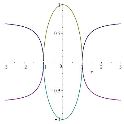
Consider the family of almost Hermitian structures (g,Jni)(g,J^{ni}) with gg determined by A1=A2=1A_{1}=A_{2}=1 and A3=xA_{3}=x. For x=±1x=\pm 1 this is the almost Hermitian structure compatible with the nearly Kähler one. In figure 1, we have depicted xx on the horizontal axis, and in the vertical axis the value of aa (as in the proof of 7). This component of the connection has the property that it is nonzero if and only if the DT instanton is irreducible, with each pair of colors corresponding to the values of aa for the different weights β\beta. Analysing this figure we see that for any value of xx, other than x=±1x=\pm 1 the DT-instantons are irreducible. When x=±1x=\pm 1, i.e. when the metric is the nearly Kähler one, these become obstructed and reducible to one of the Abelian pHYM connections in proposition 6.

Refer to caption
Figure 1. With JniJ^{ni} and A1=A2=1A_{1}=A_{2}=1, A3=xA_{3}=x.
Example 5.

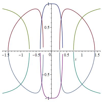
Now consider the family of almost Hermitian structures (g,Jnk)(g,J^{nk}) with gg determined by A1=xA_{1}=x, A2=10x3A_{2}=10x^{3} and A3=1A_{3}=1. In figure 2 we produce a similar plot as in the previous case. In this case we see that there are irreducible DT-instantons for any value of the parameter xx.

Refer to caption
Figure 2. With JniJ^{ni} and A1=xA_{1}=x, A2=10x3A_{2}=10x^{3}, A3=1A_{3}=1.

Appendix A The topology of the bundles PβP_{\beta}

Recall that the bundles PβP_{\beta} are constructed via Pβ=SU(3)×(T2,λβ)SO(3)P_{\beta}={\rm SU}(3)\times_{(T^{2},\lambda_{\beta})}{\rm SO}(3), where

λβ=diag(ei2β,ei2β)SU(2)/2.\lambda_{\beta}=\mathrm{diag}(e^{\frac{i}{2}\beta},e^{-\frac{i}{2}\beta})\in{\rm SU}(2)/\mathbb{Z}_{2}.

Let Vβ=Pβ×SO(3)3V_{\beta}=P_{\beta}\times_{SO(3)}\mathbb{R}^{3} be the vector bundle associated with respect to the standard representation SO(3)SO(3)-representation, and consider the U(2){\rm U}(2) bundle

Eβ=SU(3)×(T2,λ~β)2,E_{\beta}={\rm SU}(3)\times_{(T^{2},\tilde{\lambda}_{\beta})}\mathbb{C}^{2},

where

λ~β=diag(eiβ,0)U(2),\tilde{\lambda}_{\beta}=\mathrm{diag}(e^{i\beta},0)\in{\rm U}(2),

and the ismorphism. This has the property that the U(2){\rm U}(2)-adjoint bundle of EβE_{\beta} splits as 𝔲Eβ¯Vβ\mathfrak{u}_{E_{\beta}}\cong\underline{\mathbb{R}}\oplus V_{\beta} and

w2(Vβ)=c1(Eβ)mod2,p1(Vβ)=c1(Eβ)24c2(Eβ).w_{2}(V_{\beta})=c_{1}(E_{\beta})\mod 2,\ \ \ p_{1}(V_{\beta})=c_{1}(E_{\beta})^{2}-4c_{2}(E_{\beta}).

We shall now compute the Chern classes of the bundles EβE_{\beta} using Chern-Weyl theory. For this we must equip EβE_{\beta} with a connection which we choose to be the standard invariant connection given by

Aβ=βdiag(i,0).A_{\beta}=\beta\otimes\mathrm{diag}(i,0).

This has curvature Fβ=dβdiag(i,0)F_{\beta}=d\beta\otimes\mathrm{diag}(i,0) and so

c1(Eβ)=12π[dβ],c2(Eβ)=14π2[dβ][dβ].c_{1}(E_{\beta})=-\frac{1}{2\pi}[d\beta],\ \ c_{2}(E_{\beta})=\frac{1}{4\pi^{2}}[d\beta]\cup[d\beta].

Furthermore, a computation using the Maurer-Cartan equations shows that

dβ12+dβ22+dβ1dβ2=dIm((η1+iθ1)(η1+iθ1)(η1+iθ1)),d\beta_{1}^{2}+d\beta_{2}^{2}+d\beta_{1}\wedge d\beta_{2}=d\mathop{\mathrm{Im}}((\eta_{1}+i\theta_{1})\wedge(\eta_{1}+i\theta_{1})\wedge(\eta_{1}+i\theta_{1})),

and so in H4(𝔽2,)H^{4}(\mathbb{F}_{2},\mathbb{Z}) we have

[dβ1][dβ2]=[dβ1][dβ1][dβ2][dβ2].[d\beta_{1}]\cup[d\beta_{2}]=-[d\beta_{1}]\cup[d\beta_{1}]-[d\beta_{2}]\cup[d\beta_{2}].

So, writing β=kβ1+lβ2\beta=k\beta_{1}+l\beta_{2} we compute that

w2(Vβ)=12π(k[dβ1]+l[dβ2])mod2,w_{2}(V_{\beta})=-\frac{1}{2\pi}\left(k[d\beta_{1}]+l[d\beta_{2}]\right)\mod 2,

while

p1(Vβ)\displaystyle p_{1}(V_{\beta}) =\displaystyle= 14π2[dβ][dβ]\displaystyle\frac{1}{4\pi^{2}}[d\beta]\cup[d\beta]
=\displaystyle= 14π2(k2[dβ1][dβ1]+2kl[dβ1][dβ2]+l2[dβ2][dβ2])\displaystyle\frac{1}{4\pi^{2}}\left(k^{2}[d\beta_{1}]\cup[d\beta_{1}]+2kl[d\beta_{1}]\cup[d\beta_{2}]+l^{2}[d\beta_{2}]\cup[d\beta_{2}]\right)
=\displaystyle= 14π2(k(k2l)[dβ1][dβ1]+l(l2k)[dβ2][dβ2]).\displaystyle\frac{1}{4\pi^{2}}\left(k(k-2l)[d\beta_{1}]\cup[d\beta_{1}]+l(l-2k)[d\beta_{2}]\cup[d\beta_{2}]\right).

In particular, when β\beta is one of the roots r1r_{1}, r2r_{2}, r3r_{3} we respectively obtain

w1(Pr1)=12π[dβ1]mod2,p1(Vr1)=34π2[dβ1][dβ1],\displaystyle w_{1}(P_{r_{1}})=-\frac{1}{2\pi}[d\beta_{1}]\mod 2,\ \ \ p_{1}(V_{r_{1}})=-\frac{3}{4\pi^{2}}[d\beta_{1}]\cup[d\beta_{1}],
w1(Pr2)=12π[dβ2]mod2,p1(Vr2)=34π2[dβ2][dβ2],\displaystyle w_{1}(P_{r_{2}})=\frac{1}{2\pi}[d\beta_{2}]\mod 2,\ \ \ p_{1}(V_{r_{2}})=-\frac{3}{4\pi^{2}}[d\beta_{2}]\cup[d\beta_{2}],
w1(Pr3)=12π([dβ1][dβ2])mod2,p1(Vr3)=14π2(3[dβ1][dβ1]+3[dβ2][dβ2]),\displaystyle w_{1}(P_{r_{3}})=-\frac{1}{2\pi}\left([d\beta_{1}]-[d\beta_{2}]\right)\mod 2,\ \ \ p_{1}(V_{r_{3}})=\frac{1}{4\pi^{2}}\left(3[d\beta_{1}]\cup[d\beta_{1}]+3[d\beta_{2}]\cup[d\beta_{2}]\right),

so these three bundles are all topologically different.

References