The drainage of glacier and ice sheet surface lakes
Abstract
Supraglacial lakes play a central role in storing melt water, enhancing surface melt, and ultimately in driving ice flow and ice shelf melt through injecting water into the subglacial environment and facilitating fracturing. Here, we develop a model for the drainage of supraglacial lakes through the dissipation-driven incision of a surface channel. The model consists of the St Venant equations for flow in the channel, fed by an upstream lake reservoir, coupled with an equation for the evolution of channel elevation due to advection, uplift, and downward melting. After reduction to a ‘stream power’-type hyperbolic model, we show that lake drainage occurs above a critical rate of water supply to the lake due to the backward migration of a shock that incises the lake seal. The critical water supply rate depends on advection velocity and uplift (or more precisely, drawdown downstream of the lake) as well as model parameters such as channel wall roughness and the parameters defining the relationship between channel cross-section and wetted perimeter. Once lake drainage does occur, it can either continue until the lake is empty, or terminate early, leading to oscillatory cycles of lake filling and draining, with the latter favoured by large lake volumes and relatively small water supply rates.
1 Introduction
Large areas of the Greenland ice sheet experience surface melt water drainage [1], while surface drainage is confined to lower elevations in Antarctica [2, 3, 4]. Surface melt drives the evolution of subglacial drainage system in Greenland [5, 6, 7], which in turn controls sliding speed [8, 9, 10, 11]. Accumulation of surface water can also enhance surface melting by reducing albedo [12, 13] and cause the break-up of floating ice shelves [14, 15, 16, 17], while the injection of surface melt under a floating ice tongue can drive convection in fjords [18, 19], and enhance as well as localize melting at the base of the ice tongue [20, 21].
Lakes situated in local depressions on the ice surface are common features of drainage systems in both, Greenland and Antarctica. These lakes store water, enhance surface melt and, in the case of Greenland, can cause short-lived acceleration of ice flow through abrupt drainage to the bed by hydrofracturing [8, 22, 23, 24]. Much research has focused on the latter effect, even though a significant fraction of surface lakes in Greenland either drain slowly or not at all [1, 25, 26, 27, 28, 29], while there are no known surface lakes on the grounded part of the Antarctic ice sheet that drain to the bed [30].
Motivated by field observations made in Antarctica [31], we consider the case of lakes draining purely through channels incised into the surface of a grounded ice sheet (as opposed to a floating ice shelf). The observations in question specifically suggest that a surface lake on a grounded portion of the ice sheet may be capable of draining through a near-surface channel incised into the ice in the absence of any significance forcing (that is, at the end of winter) after a lengthy period of apparently steady lake filling levels. While similar overland drainage may also be relevant to higher elevations in Greenland [28], where few lakes drain through hydrofracture [1], we neglect seepage into a firn aquifer in our work [32, 33], which may be relevant for some of these Greenlandic lakes.
There have only been a handful of attempts to model lake drainage along glacier and ice sheet surfaces through thermal erosion of a channel through an ice dam [34, 35, 36, 37, 38, 39]. Most of these consider drainage along more steeply-angled glacier surfaces, where flow is likely to be Froude supercritical. In all of these previous studies except Kingslake et al. [38], surface lakes are considered as natural hazards, with the ultimate aim of computing hydrographs for rapid surface drainage. In addition, and by contrast with models for drainage along the glacier bed [40, 41, 42, 43, 44, 45, 46] none of the surface drainage models listed resolve channel incision (and therefore channel slope) as a function of position along the flow path, but instead take the form of ‘lumped’ models intended to describe conditions near the channel intake only.
Although the model we develop is in principle applicable to the outburst floods studied previously, our main goal differs substantially from these prior studies. We are interested primarily in whether water input to a lake, causing the lake to overflow, necessarily leads to lake drainage by channel incision, and whether drainage can be partial or must continue until the lake basin is completely empty. As a result, we focus on systems in which incision of the channel is quite slow, and competes with horizontal advection and vertical uplift of the ice surface due to the flow of the ice sheet over bed topography. These latter two processes are responsible for shaping the surface depression occupied by the lake to begin with [47], but have rarely been considered in the context of surface lake dynamics [48] and are not incorporated in the existing models for rapid lake drainage. Among other consequences, the incorporation of advection forces us to employ a partial differential equation-based model, resolving position along the channel as well as time.
Our model bears close resemblance to so-called stream power models for fluvial landscape evolution in non-glacial contexts [49]. The latter typically incorporate uplift [e.g. 50, 51, 52], but the additional effect of horizontal advection is not commonly considered as part of fluvial landscape evolution. It is however key to studying supraglacial lake evolution: while incision due to erosion (or in our case, melting) leads to a backward-propagating steepening of the channel bed, advection simultaneously moves the steepening bed in a forward direction. In the absence of that forward advection, a lake at the upstream end of the channel will invariably be breached by channel incision if there is a non-zero water supply, but this is not the case in the presence of advection.
The paper is organized as follows: In §2.1 we define a basic model consisting of the St Venant equations for a surface stream coupled with an evolution equation for channel depth, based on local dissipation driving channel incision. In §2.2–2.4, the model is reduced based on a small ratio of water depth in the channel to lake depth, and water velocities being much larger than ice velocities, while local Froude number is assumed to remain subcritical. This results in a nonlinear hyperbolic evolution equation for channel evolution [49], coupled to an evolution equation for lake volume (§3.1). The formation of shocks in the model and how they control discharge from the lake is studied in §3.2–3.4, with boundary layer solutions of the full model around the shocks relegated to appendices A–B. Numerical solutions by the method of characteristics (appendix D) are given in §4, where we show that lake drainage occurs above a critical value of water supply to the lake (§4.2), which can result in either in complete lake drainage or oscillatory cycles of lake drainage and refilling (§4.3).
2 Model
2.1 Model Formulation
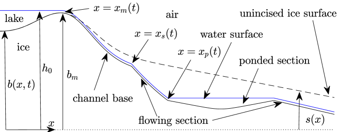
We consider a surface melt water stream with cross-sectional area , with the base of the stream channel at an elevation , and the velocity in the stream being . Let be distance along the stream and time, and let , and depend on and (figure 1). Assuming a Darcy-Weisbach law governing shear stress at the walls of the channel, we express conservation of mass and momentum using a St Venant model as [e.g. 53, chapter 4]
| (1a) | ||||
| (1b) | ||||
| where subscripts and denote partial derivatives, is melt rate at the channel wall, expressed as an area of ice melted per unit time and unit length of channel, is the wetted perimeter of the channel and is the elevation of the water surface above the bottom of the channel. is the density of water and is a friction coefficient depending on wall roughness in the channel. Note that by equating the source term with melt rate, we ignore seepage into or out of a firn aquifer, or substantial water input from tributary streams. | ||||
To simplify matters, we assume that the cross-sectional area can grow or shrink but retains a shape determined by its size alone. Our main interest is in downward incision of the channel, which we assume to be a slow process compared with the adjustment of channel shape, since we will assume below that water depth is much less than the typical amplitude of channel elevation . Consequently, we treat and as non-decreasing functions of , whose form depends on the geometry of the cross-section. At a minimum, we know that water depth must vanish when cross-sectional area does, so .
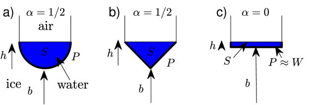
The simplest way to parameterize the cross-sectional shape of the channel is to treat it as a semi-circle (figure 2). In that case, the radius of the cross-section is and
| (1c) |
Alternatives would be to assume the channel is triangular with a fixed angle between the channel sides and the vertical
| (1d) |
or to fix a width that is much greater than water depth, and to put [as is done in 53]
| (1e) |
Generically, this suggests we consider
| (1f) |
with , , (we admit that width and therefore wetted perimeter may not depend on , but water depth must, so cannot vanish while can): (1c)–(1d) have while (1e) puts , . In fact, the examples above suggest that the product of wetted perimeter and water depth scale as the cross-sectional area, in which case , and that the exponents are not only positive but also satisfy , .
We assume that energy dissipated by the flow is instantly transferred to the wall of the channel and turned into latent heat, and that this is the dominant mechanism of channel incision. A more sophisticated model could track the temperature of the water and use a heat transfer model [see also the discussion in 54]; here we assume that heat transfer is highly efficient at the length scales under consideration. Letting be the latent heat of fusion per unit mass of water, we put
| (1g) |
the right-hand side being the rate at which work is done per unit length of channel by water moving at velocity against the friction force on the channel wall. In order to model how fast the channel cuts into the ice, we assume that downward incision can be estimated by distributing melt equally over the wetted perimeter, leading to an incision rate of . Future work will need to address both the channel shape parameterizations and the distribution of melt over the channel wall: related work on englacial channels [55] may serve as a template.
In addition, we assume that the ice surface is moving horizontally at a velocity and is subject to localized uplift or drawdown at a prescribed rate due to flow of the glacier or ice sheet over bed topography [e.g. 47], where we will later assume for simplicity that is constant in space as well as time, as is appropriate for instance for rapidly sliding ice. Then
| (1h) |
We assume that the base of the channel is incised into an ice surface at elevation , with . In assuming that is constant in time, we are assuming not only that we can ignore localized, enhanced ‘creep closure’ around a deeply incised channel [56] as well as snow accumulation at the base of the channel during winter, but also that is in steady state [47], and itself satisfies
| (1i) |
We will generally use as an initial condition, representing a channel that is only just beginning to incise into the ice surface. A modification of the present model to a dynamically evolving ice surface will be presented elsewhere.
We envisage the channel draining a reservoir at its upstream end. For simplicity, we assume that the seal point of the lake (the maximum in ) is some distance downstream of , and that we can relate lake volume directly to water level at , and put
| (1j) |
with the dot on denoting an ordinary time derivative, being a prescribed rate of inflow to the lake due to surface melting in some larger upstream catchment. is an increasing function of , dictated by the bathymetry of the lake. The bathymetry in turn is presumably determined by and , but we do not consider that in detail here, nor do we consider the possibility that surface loading due to the lake could affect the motion of the ice. As with an evolving ice surface , the latter complication will be studied in a separate paper.
Before we continue, we note some important limitations of the model. First, by assuming a fixed flow path and not modelling tortuosity, we are not considering the effect of meanders on flow and channel incision, even though meandering is known to be a common feature of glacier surface streams [e.g. 57, 58]. Second, the one-dimensional nature of the model implies not only that there is a single outflow from the lake, which is ultimately likely as two competing outflow channels are presumably prone to instability, with the larger channel persisting while the smaller is abandoned. It also implies that, if flow in the channel were to cease temporarily due for instance to seasonal variations in water supply , the same channel will be re-occupied when flow recommences. We return to this in section 5.
In addition, we also neglect surface lowering due to melt driven by insolation or a warm atmosphere, or freezing due to heat fluxes into the ice. This may be reasonable for the incision of the channel relative to the rest of the ice surface , is more questionable for the lake itself. Here, enhanced absorption of incoming radiation in the lake water is likely to lead to preferential melting of the deeper portions of the lake [see also 59]. By the same token, we also neglect the possibility that the lake water could be warmed relative to the melting point by incoming solar radiation [see also 35]. That said, by omitting externally-driven melting, our model allows us to focus purely on the coupled effects of ice and water flow in the erosion of the channel and its effect on lake drainage.
2.2 Non-dimensionalization and a reduced model
We assume that a length scale can be determined from the uplift field , and that scales for vertical and horizontal ice velocities and are also known. In terms of these, we define scales , , , and through
Our choice of scales here reflects the following: we are interested in significant channel incision over a single advective time scale for the ice surface, so that uplift, advection and incision of the channel naturally compete with each other. Given a natural surface topography , that sets a dissipation rate and therefore a water flux scale . It is possible to construct the same problem as below for a much shorter channel incision time scale, corresponding to greater dissipation and therefore water fluxes; that however precludes the generation of a lake, which requires the lake seal to be generated through uplift of the ice surface.
From these scales we obtain the dimensionless groups
| (2) |
These have straightforward interpretations: is the ratio of water depth to ice surface topography, the Froude number is the usual square root of the ratio of kinetic to gravitational energy, is the ratio of gravitational potential energy to latent heat, and is the ratio of ice to water velocity. With the possible exception of , we expect all of these parameters to be small: if water moved at speeds comparable to the ice, then surface drainage would presumably be of no interest, while the surface topography scale would have to be around 30 km with a terrestrial gravitational field 10 m s-1 in order for gravitational potential energy and latent heat J kg-1 to be comparable. We also expect the water depth in a glacially-dammed lake to be larger than the flow depth in the stream draining it, except possibly during a very rapid outburst flood or for shallow lakes.
In fact, for realistic values of m a-1, m, km, m s-2, , we obtain, with and given by (1c)
values that are realistic for surface streams with gentle slopes. With the choice of scales defined through (2), we define dimensionless variables through
| (3) |
and define
| (4) |
and also put , . Then, in dimensionless form, dropping the asterisks on the dimensionless variables immediately, the model becomes
| (5a) | ||||
| (5b) | ||||
| (5c) | ||||
Following the discussion above, we assume that , and . At leading order in these small parameters, we obtain from (5)
| (6) |
Water flux along the channel is constant in space, velocity is controlled by a balance of friction at the channel wall and the downslope component of gravity acting on the water in the channel, and the channel bottom evolves due to advection, uplift, and melting driven by local dissipation of heat in the flow of water.
The reduced model is subject to the caveat that the local Froude number remain less than unity. Where , the channel becomes unstable to bedform formation at short wavelength, while for , roll waves form in the flow (see §3 of the supplementary material, also sections 4.4.4–4.5.2 and chapter 5 of Fowler [53]). A reduced model that does not explicitly resolve these phenomena but focuses on channel incision at the larger scale may still be possible, but would presumably require a multiple scales expansion [60]. We leave this to future work.
Persisting with (6), we find that is independent of position. Hence depends on flux and slope through from (6)2 as
| (7) |
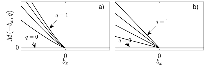
where we assume that and . With channel geometry given by (1f), specifically in dimensionless form, we obtain a dimensionless melt rate
| (8) |
The function here is monotonically increasing and convex function of for , strictly so if , and a monotonically increasing function of for (see also figure 3). Our assumptions about channel geometry can be relaxed significantly while allowing these properties to be preserved: as shown in §2 of the supplementary material, monotonicity is assured if hydraulic radius is an increasing function that vanishes when , while (strict) convexity follows if is (strictly) concave.
At face value, substituting in (6)3 yields the single evolution equation for ,
| (9) |
Note that this is effectively the stream power equation for landscape evolution in [49, 52, 61], with some alterations as explained in section 3.1.
Our assumption that is however not always satisfied. Where such reverse slopes occur, the reduced model breaks down: water depths become large, flow velocities become small and melt rates vanish at leading order, and we put if to account for this. That in itself does not however suffice, since reverse slopes can induce ponding even on downward slopes further upstream. We deal with this next.
2.3 Ponding
Formally, the dynamics of a ‘ponded section’ of channel (where, once more, water is deep while surface slope, velocity and melt rates are small, see figure 1) can be captured formally by a rescaling as described in appendix A. Without engaging in that formalism, assume that water storage in the ponded sections remains negligible, so that we can treat flux as constant throughout the domain; this turns out to require . When there is flow with , then a ponded section comprises those points that lie below the high point or ‘seal’ in the channel bed at its downstream end, since the nearly flat water surface in the ponded section cannot exceed that seal height significantly. Hence the union of all ponded sections is the set , which necessarily encompasses reverse slopes , but will generally also include stretches of channel with a downward-sloping bed .
If no water is flowing and , actual ponded sections with standing water may be smaller. The purpose of identifying ponded sections is however mostly to impose an absence of melting there, and with , we obtain regardless of whether we have identified ponding correctly. The appropriate modification of (9) to account for ponding is therefore via a ‘ponding function’ ,
| (10a) | ||||
| (10d) | ||||
Note once more that the introduction of the ponding function is redundant where in ponded sections, since in that case by definition.
2.4 Outflow at the lake
As we have to revisit the non-dimensionalization of the problem, we temporarily reintroduce asterisks on dimensionless variables. We assume that the lake at exists because it is upstream of a ponded section with a reverse slope. Let be dimensionless water depth in that ponded section, scaled with ice surface topography (as is appropriate for ponded sections, see appendix A). Also let be the water level of the lake. We define a dimensionless lake volume function and a dimensionless water supply function through
| (11) |
where the variables on the right-hand sides of both equalities are dimensional. We assume formally that and are functions. By this, we mean that lake volume is comparable to (or less than) the volume typically carried by the channel in a single channel evolution time scale , and inflow into the lake is comparable with or less than the flux scale that causes significant channel incision over the advective time scale of the ice.
We immediately revert to dropping asterisks on dimensionless variables. As in the previous section, water surface elevation must be constant up to the lake seal (the end of the ponded section that extends downsteam from ), Water surface elevation also cannot exceed seal height at leading order (appendices A and B.2). Consequently, we find that water depth at the upstream end of the domain is either at the height of the seal point if water is flowing, or below that seal height if no water is flowing. We denote the seal height by , so that
| (12a) | |||
| Similarly, we will use to denote the seal location, . | |||
With constant throughout the domain, water balance of the lake can therefore be written as
| (12b) | ||||
| (12e) |
where is storage capacity in the lake and overdots again denote time derivatives. Flux in the channel is the difference between inflow into the lake and the rate at which water is retained in the lake, and the latter is controlled by how the high point in the channel itself evolves due to uplift, advection, and incision.
3 Solution
3.1 Characeristics
If we treat and momentarily as known, then (10a) can be recognized as being of Hamilton-Jacobi form [49],
| (13) |
where the Hamiltonian is given by
| (14) |
replacing (itself a function of and ) with for clarity in the meaning of derivatives of .
The method of characteristics [62, §3] allows us to write the solution to (10a) as follows: we define characteristics as curves of constant in the transformation given by
| (15) |
where is the partial derivative of with regard to its third argument, with , and all treated as functions of and , while is the partial derivative of with respect to its first argument. Along a given characteristic, and evolve as
| (16) |
subject to the given initial and boundary conditions. We take these to be at and at , so elevation at the upstream end of the domain remains constant throughout. Note that we do not attempt to differentiate the piecewise constant function when forming in equation (16). Instead, we regard discontinuities in as potential shocks, and treat them separately.
As already pointed out, the problem (13)–(14) is structurally very similar to ‘stream power models’ for landscape evolution [49]. Aside from complications due to the ponding function , the main differences between our model and canonical stream power models is the way that water flux is controlled by lake drainage, and the fact that the Hamiltonian here remains convex in the slope variable , but need not be monotonically decreasing due to the advection term. As a result, characteristics and shocks can travel downstream as well as upstream, with major implications for breaching the seal of the lake and controlling the flux .
We give a comprehensive account of shocks and discontinuities in below Figure 4 provides an overview of the different possibilities. We treat the majority of cases in sections 3.2–3.3 and derive formulae for flux in terms of shock geometry at the lake seal in section 3.4. We relegate the analysis of the upstream end of ponded sections to appendix C, where we show that the discontinuity in at such a location cannot generate a shock but may give rise to an expansion fan rather. The material below is fairly dense and, at this stage, abstract. On a first reading, it may be preferable to skip to section 4 to understand the zoology of features of the solution before filling in the theoretical background in sections 3.2–3.4 and appendix C.
3.2 Shocks in a flowing section
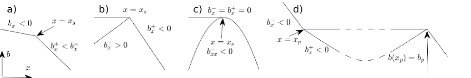
Equation (13) breaks down when characteristics intersect at shocks. Intersections require characteristics to travel faster upstream of the seal than downstream. The melt rate is convex in slope , and for on either side of a shock in a flowing section, so is the Hamiltonian . Denoting by superscripts + and - limits taken from above and below the shock at , respectively, we must have for a shock in a flowing section (figure 4(a)). These shocks represent ‘knickpoints’ in standard geomorphological parlance [49, 51].
We require that remain continuous across any shock or discontinuity in (see appendix B for the boundary layer structure of the full model around the different types of shock). Differentiating both sides of with respect to , we obtain , where the overdot denotes differentiation with respect to time. Equivalently (see also Royden and Perron [51])
| (17) |
where of course for a shock in a flowing section; we retain and for later convenience. By the mean value theorem, a strictly convex corresponds to somewhere between the characteristic velocities on either side, with characteristics terminating at the shock from both sides as expected. In fact, knickpoint shocks between two parts of a flowing section can occur only if in (8), so are strictly convex for : for , the characteristic velocity in a flowing section is independent of slope and characteristics do not cross.
3.3 The downstream end of a ponded section
Shocks between a ponded section upstream and a flowing section downstream (, , , , see figure 4(b)) are structurally equivalent to knickpoint-type shocks. Equation (17) still holds, where now ; the discontinuity in is in fact a red herring her since for anyway (this differs from the upstream end of a ponded section in appendix C, where the discontinuity in is crucial). The important distinction with the knickpoint shocks of section 3.2 is that shocks between ponded and flowing sections can form even if is not strictly convex (that is, for ), since the characteristic velocity upstream of the shock is larger than its counterpart downstream, and characteristics terminate at the shock from both sides.
The seal of the lake may take the form of a shock between ponded and flowing, and its motion then controls the flux as described in section 3.4 below. We refer to ‘breaching’ of the seal as incision into a seal that was previously in steady state, leading flux to increase and the lake to drain, and this requires a shock to pass the steady seal location as we will show in §4.
The transition from ponded to flowing need not correspond to a shock, however. A continuous slope with is possible if the transition point is a local maximum of such that characteristics enter from one side and exit on the other, with no jump in or , and with a continuous melt rate and Hamiltonian (figure 4(c)). Differentiating with respect to time and differentiating (10a) with respect to , so with and with , we obtain
| (18) |
Since the ponded section is upstream and is a maximum of , we have and . There are two cases, with negative and positive at the seal, respectively. Positive corresponds to rapid downslope motion of the seal with ; this does not occur except for contrived initial conditions.
Assume therefore that , so . Characteristics upstream of travel at speed , so a smooth slope requires characeteristics to emerge on the downstream side, where the characteristic speed is , with indicating the limit taken as is approached from below. Requiring so that characteristics exit downstream, a smooth slope is possible provided
| (19) |
Importantly, this type of smooth seal can correspond to a steady state. The steady state seal location is defined by with . In steady state, upstream of the seal, which ensures that at the seal as required, while differentiating both sides yields , so as needed for a steady state.
It is instructive to ask when (19) can be violated. For given by equation (8), if , and (19) will not be violated provided and . By contrast, for , and (19) can be violated for sufficiently large fluxes . In practice, this implies that shocks breaching the seal form downstream of the seal for and migrate upstream, while for , such knickpoint shocks cannot form and shocks that breach the seal form at the seal itself when .
3.4 The computation of flux
Key to the model is to understand how flux evolves, which requires the evolution of the seal point height in (12e). There are two scenarios: either the seal point is a shock, in which case from (17)
| (20) |
or the seal is a smooth transition point, and with at such a smooth transition,
| (21) |
We can now compute flux . Assuming lake level is equal to seal height with , (12e) leads to
| (22) |
if there is a shock and (20) holds, or if the seal is smooth. Here, is simply the base outflow rate that results if there is no incision into the seal due to melting.
Only the case (22) of a shock at the seal is non-trivial. Any positive outflow rate satisfies
| (23) |
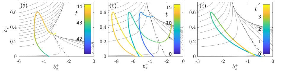
For and , the function defined in equation (8) is an increasing, concave function of with . With and for a shock at the seal, it follows that the left-hand side of (23) vanishes at , decreases for small , reaches a global minimum and then increases thereafter (figure 5(a)). If the base outflow rate is positive, there is then a single positive root for , where increases with base outflow rate and with storage capacity (for fixed base outflow rate). For , the solution for can become multivalued: is a valid solution of the original problem (22), but there are in addition two non-zero solutions if is larger than the global minimum with respect to of the left-hand side of (23) (figure 5(a)). For the melt rate given by (8), that situation arises when
| (24) |
For even more negative , is the only solution. The multivalued solution in that case results from the fact that the incision rate due to sufficiently large flux can overcome an uplift rate that on its own is sufficient to re-seal the lake, and thus maintain that flux.
To resolve the multivaluedness of properly, we have to go to higher order and compute the difference between water level in the ponded region and seal height at leading order. Doing so requires solving a boundary layer problem around the seal as described in appendix B.2 or, in more detail, in sections 1.5–1.6 of the supplementary material. We obtain a regularized version of (12)
| (25) |
Note that this replaces the cruder but structurally similar ordinary differential equation models for lake surface lowering in Raymond and Nolan [35], Kingslake et al. [38] and Ancey et al. [39]. The function , is zero when the first argument is non-positive, and has an derivative with respect to its first argument when the latter is positive. We also assume that the derivative is positive, since we expect a higher water level relative to the seal to lead to a larger flux. This property is confirmed numerically in appendix B.2 and can presumably be proven mathematically, although we have not tried.
Putting , we recover (12) at leading order, with the flux implicitly defining the correction . The latter however represents a steady state solution of a transient that occurs at a faster, time scale: substituting for from (20) and rescalng in (25) yields
| (26) |
with and constant on the fast time scale. will evolve to a pseudo-steady state that satisfies either (23) or , and which is stable in time to small perturbations in . The latter constraint implies that, when there are three solutions to (23), only the largest solution (for which again increases with base outflow rate ) and the zero solution are viable as indicated by solid lines in figure 5(a). In addition, the relevant, stable solution branch of the original leading-order model (12) is chosen by continuity of in time whenever such continuity is possible: this is true at least provided there are no significant variations in on the short time scale over which the lake level correction adjusts. In practice, this could be a real consideration with diurnal water input fluctuations. Presumably these are generally insufficient in practice to lead to changing significantly, and do not affect the outflow rate , but a more sophisticated approach is necessary if they do.
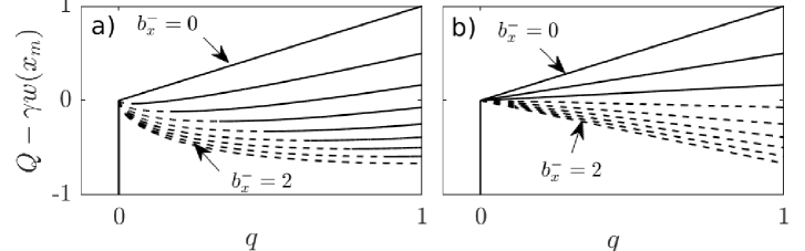
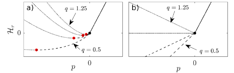
For the commonly encountered situation of the upstream side of the lake seal being in steady state, , we can use the stability result to visualize flux as a multi-valued function of and in the limit of small (figure 6(a)). Here a zero solution is possible everywhere above the red dash-dotted line , and becomes the only solution in the area demarcated by a solid black curve. Flux is not continuous across either of those boundaries when transitioning between solution branches. Note also the region bounded to the left by the dashed black contour: here the non-zero flux is less than the inflow , with the seal advancing and rising in height, but water still flowing out of the lake.
For , the situation is more complicated: we have and hence (23) reads
| (27) |
Stability again requires to increase with , so the coefficient of on the left must be positive if is non-zero, leading to a solveability condition when . By contrast, a unique, stable solution exists when (figure 5(b)). That, however, potentially leaves a region of the plane with no viable solution, since we may have while the solvability condition is violated.
We can again visualize this situation, plotting flux for as a function of and if (figure 6(b)). Unlike the case , is now not multivalued, but instead undefined in a ‘forbidden’ part of the plane if as shown, reflecting the solvability condition.
As a result, breakdown of the model is a very real possibility if . If the seal migrates backwards with a steepening upstream slope, can approach the critical value at which the coefficient in (27) vanishes, and undergoes runaway growth (as the red boundary of the forbidden region is approached from below in figure 6(b)). Physically, incision into the seal becomes fast enough in the forbidden region that the flux out of the reservoir cannot keep water level close to the seal height (appendix B.2): a finite (but presumably short-lived) jump in water height across the seal will evolve, with very large flux and incision rates that cannot be captured by our reduced model. The lake drains abruptly, and a rescaling of water depth in the channel is required to capture this phenomenon.
4 Results
4.1 Lake drainage modes for steady water supply
We solve (10)–(12) numerically using the method of characteristics with a backward Euler step as described in appendix D. We use the regularized flux prescription (25) for , and at times for in order to explore what happens ‘beyond’ the model failure identified at the end of the last subsection. When we do use (25), we treat simply as a regularization rather than trying to emulate the function shown in figure 17(b). Consequently we drop the slopes and as arguments from . In practice, we use , and put .
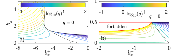
Figures 7–11 illustrate the behaviour of lakes that are initially empty with , where is the unincised ice surface, satisfying . This initial profile is a steady state solution in the absence of flowing water, and the profile therefore remains unchanged until the lake is full: only then does water begin to flow and the channel becomes incised on the downstream side of the lake seal. We compute results for an uplift velocity of the form
with , , and ; this results in a steady state surface in the form of a Gaussian superimposed on a uniform downward slope (see e.g. the top profile in figure 7(a1–a2)). The choice of ensures that at , so that the upstream end of the domain is the bottom of the lake. The steady state surface is shown as a dashed black line in figure 8(a2), or as one of the black curves in figure 7, panels a1 and a2. An alternative form of that asymptotes to a negative limiting value from above for large negative (meaning, the lake bed does not flatten out above the seal) is explored in section 4.2 the supplementary material.

We use two different choices of shape exponent, (the fixed-width slot of equation (1e)) and (the semicircles and triangles of equations (1c) and (1d)). For each of these, we compute solutions for different constant values of water input and of storage capacity , treating the latter as independent of water level [see also 42, for a discussion of lake hypsometries]. Both of these assumptions are simplistic, but help understand the dynamics of surface lakes more clearly. Importantly, real ice sheet surface lakes are subject to time-dependent forcing due to seasonal and shorter melt cycles. In many cases, that forcing is quite rapidly varying, since the time scale for ice to traverse the length scale of the seal may be quite long: with m yr-` and 1 km, one unit of dimensionless time here corresponds to ten annual melt cycles. We explore the effect of rapidly varying water input in §5.1 of the supplementary material, where we find that it leaves the qualitative behaviour of the system largely unchanged. Here we persist with a constant water input in order to illustrate that qualitative behaviour more cleanly.
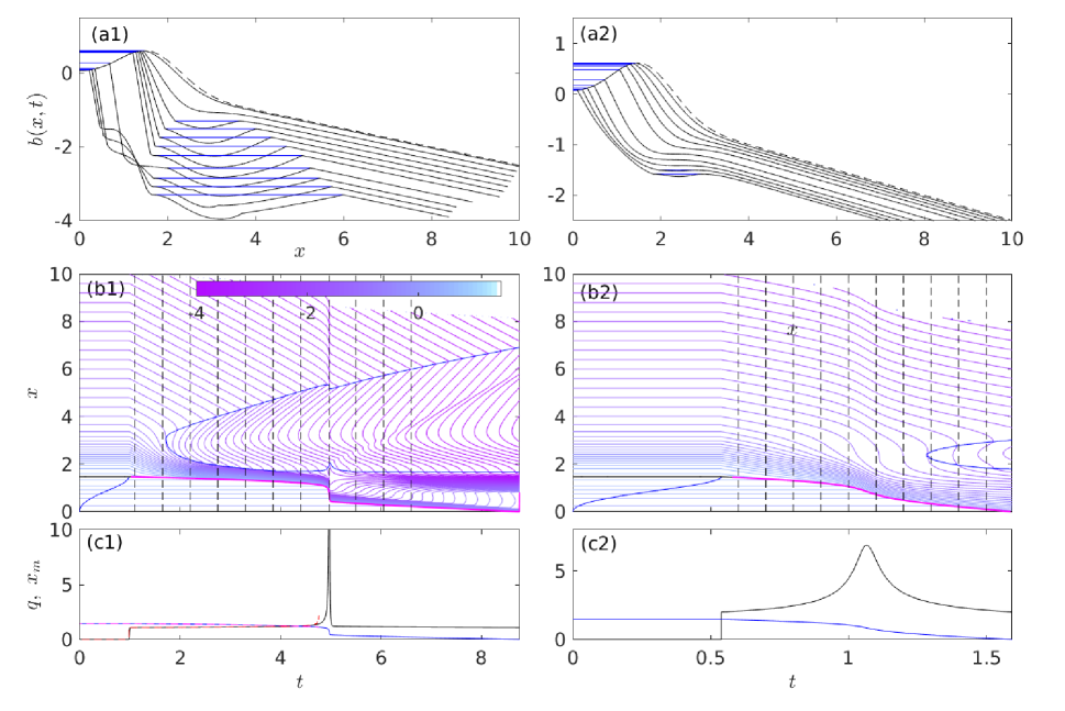
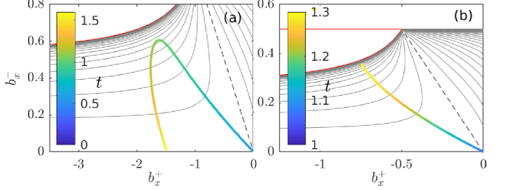
Depending on the values of , and , different outcomes are possible, differentiated at the coarsest level by whether the lake drains or not. Figure 7 illustrates two possible end members for . In both cases, outflow from the lake commences once water level (blue curve in panel b) reaches the smooth seal (black line in panel b). For the low-flux example in column 1, with , the smooth seal (the maximum in the unincised ice surface at ) remains in place, and hence (with at the steady seal), from the paragraph following equation (22). The channel steepens downstream, but no backward-migrating shock forms. The steepened flowing section terminates in a ponded section that migrates downstream, eventually leaving the entire domain in a new steady state.
Column 2 shows a high-flux counterexample to the steady state of column 1, with and . Here a shock forms quickly: the inset in panel b2 shows that the shock (magenta) forms downstream of the smooth seal (black) as predicted at the end of section 3.3, and subsequently migrates upstream to breach the lake. This causes flux to increase as stored lake water is released. The dowstream side of the shock steepens and a ponded section again forms further downstream. Although the steepening on the downstream side of the seal is eventually reversed (panel a2), the backward migration of the shock continues until the lake is fully drained.
Note that we may naively attribute the steepening of slopes near the smooth seal location in both columns of figure 7 to melting after outflow from the lake commences. Characteristics offer a different perspective that will be important later: slope evolves as along characteristics, that is, as the result of differential uplift. Melt enters into the evolution of slope by determining how fast a given characteristic propagates, with by (15). Larger fluxes lead to increased and hence to reduced characteristic velocities. The steepest downward slopes result when is near zero where the uplift rate derivative is most negative (which is indeed near the smooth seal location), causing characteristics to linger. That does not occur at the largest fluxes , however, since then becomes progressively more negative. The latter effect, of large discharge flattening slopes, is evident in column 2 of figure 7, where slopes downstream of the shock become less steep as the shock approaches the upstream end of the domain. This flattening of downstream slopes will play a key role in section 4.3 below.
As a further aside, note that we choose not to introduce new characteristics at the bottom end of the domain when the characteristic velocity there is negative, as in figure 7(b2), where the contour plot is blank in the top right-hand corner. Adding characteristics would require an additional boundary condition, the choice of which however should not affect lake drainage unless the characteristics introduced there reach the lake seal.
Depending on storage capacity , more complex behaviour can occur at intermediate values of water supply as illustrated in figure 8. The left-hand column shows a higher storage (, ) example, the right a lower storage (, same ) case.
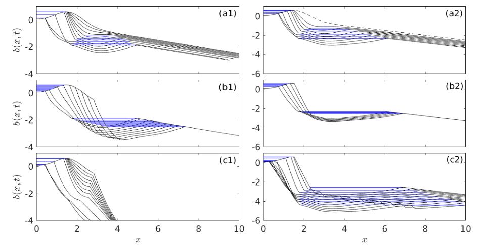
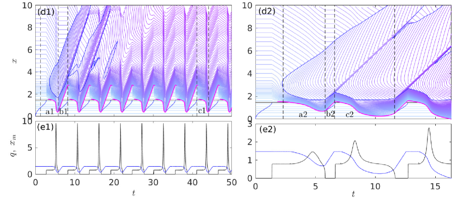
For the former, we see periodic oscillations being generated. As in column 2 of figure 7, a shock forms downstream of the smooth seal, steepening initially and breaching the lake. Lake drainage does not continue to completion, however. The seal stops migrating upstream before reaching the low point of the lake, with slopes downstream of the seal again flattening some time after the lake seal has been breached (panel a1). Outflow stops and the shock is advected downstream, allowing the initial steady state surface profile to re-establish itself and re-forming a smooth lake seal. The shock that caused the original drainage event migrates some distance downstream before the lake refills and outflow starts afresh (panel b1). Panel d1 shows that a new shock (break in the magenta curve) forms and repeats the drainage of the lake, with the channel profile in the entire domain undergoing periodic oscillations after several cycles of lake drainage and refilling (panels c1, e1).
For the lower storage case of column 2 in figure 8, we again see a shock breaching the seal, partially draining the lake and then stopping, with slopes downslope of the shock initially steepening and then flattening. The shock is again advected downstream and a smooth seal re-forms, but the refilling of the lake occurs more rapidly. The same shock that originally breached the lake is reactivated and breaches the seal again, this time migrating further upstream. The lake fully drains during the third such drainage cycle. We return in section 4.3 to a more detailed analysis of the mechanism by which lake drainage becomes oscillatory, and of the differences between the two cases in figure 8.
The range of drainage styles observed for is more limited. At low water input , the channel develops into a steady state in much the same way as shown in figure 7, column 1. At larger , a shock once more forms, although this time at the seal in agreement with sections 3.2–3.3. The outcome of that shock migrating backwards into the lake leads to flux increasing and one of two outcomes, shown in figure 9.
Column 1 shows a case with more moderate water input and . Panel c1 shows results for discharge and seal position from two computations: one without the regularization advocated in equation (25) (magenta and red), and one that is regularized (black and blue). The unregularized model has a singularity in finite time, as expected from the results in section 3.4 (see in particular figure 6(b)): this manifests itself in a very rapid rate of increase followed by the Newton solver used to compute backward Euler steps failing to find a solution.
The regularized solution instead undergoes very rapid drainage at a slightly later time (), the timing being different because the regularization in question involves water level in the lake having to rise further to reach the same flux. The singularity in flux in the unregularized model is averted because he regularized model allows water level to differ significantly from seal height : consequently lake drainage can lag behind the rapid lowering of the seal that occurs for . That being said, seal incision continues after the very rapid drainage, and lake drainage continues to completion as in column 2 of figure 7.
Column 2 of figure 9, at a larger inflow rate than column 1, shows a much more straightforward analogue to column 2 of figure 7, with seal incision leading to a peak in flux and continued seal incision until lake drainage is complete, without a (near-) singular peak flux. Importantly, we did not find instances of oscillatory lake drainage for .
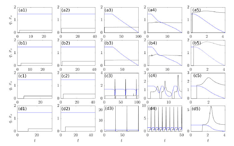
A more systematic exploration of the effect of changing storage capacity and water input is shown in figure 10 for and figure 11 for , where we use the unregularized version of the model for the latter. In both cases, inflow rate alone determines whether the seal is breached, with the results suggesting that a critical value of separates solutions that experience at least partial lake drainage from those that leave the seal intact. The fact that the initial seal breach does not depend on storage capacity is trivial: until a backward-migrating shock has formed and breached the seal, the intact, steady-state smooth seal leads to outflow balancing inflow once the lake has filled, with , and the shock that breaches the seal must form at that value of flux .
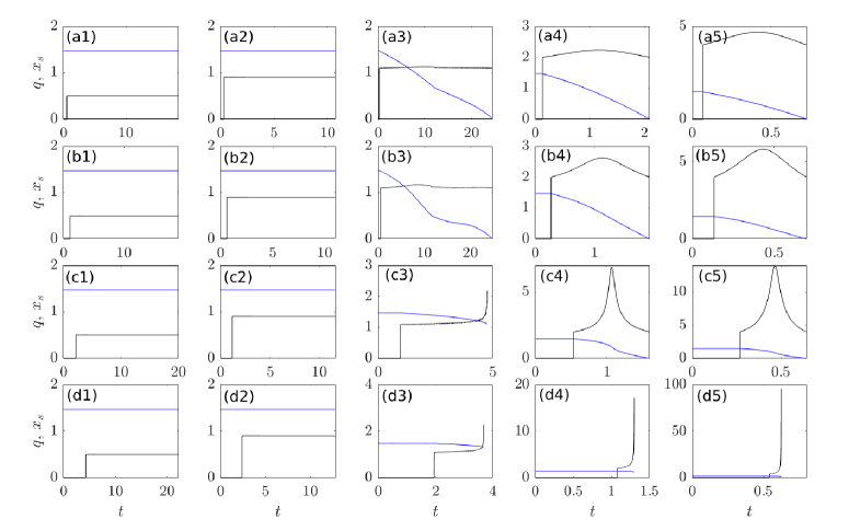
Once the seal is breached, the outcome of lake drainage depends on both and . As already indicated above, for , moderate and larger favour oscillatory drainage of the lake, with smaller and larger ultimately also leading to periodic oscillations rather than divergent oscillations eventually leading to lake drainage. For , smaller and larger by contrast favour blow-up of the solution with singular outflow ; oscillatory lake drainage does not occur in any of the computations we have performed.
4.2 Criteria for lake drainage
For constant water input to the lake with in steady state upstream of the seal, there appears to be a critical value of above which a shock either forms at the seal (if ) or below the seal (if ). The shock migrates backwards, leading to at least partial lake drainage.
Below, we identify breaches of the seal with parameter combinations for which there is no steady state solution to (10)–(12), since steady states are naturally the solution for large times if the lake seal is not breached. To see that steady states are a natural consequence of the seal remaining intact, note that the upstream end of the domain has constant , and hence there. If the seal is not breached and is therefore constant, then the value of the Hamiltonian remains constant along any characteristic that does not cross the upstream end of a ponded section. Specifically, denote by the value of the Hamiltonian as a function of the characteristic variables, so
| (28) |
and is constant if is. Note that equation (28) holds except possibly where a changes discontinuously along a characteristic, which is possible only at the upstream end of a ponded section (see appendix C).
From (28) and at , it follows that any point on a characteristic that originates at the upstream end of the domain is also in a local steady state with , provided the seal remains steady and is therefore constant. This behaviour is evident in column 1 of figure 7, where steady state conditions are established progressively down-flow as characteristics that cross the seal after lake outflow has commenced propagate downstream across the domain, with the ponded region progressively moving down-flow as well.
To avoid the difficulties associated with such ponding downstream of the lake seal, we assume below and in the supplementary material that at the upstream end of the domain, creating the lake seal in the first place, with a single root defining a steady-state seal location , and downstream of that. All computational results presented above conform to these restrictions: the corresponding unincised surfaces , defined by , have single maxima (see e.g. figure 8(a2)).
In that case, a global steady state results if the characteristics crossing a steady seal can fill the entire domain, while non-existence of steady states implies that such characteristics cannot propagate through the entire domain. As we argue in §4 of the supplementary material, some characteristics from below the seal must then propagate upstream instead, and cause a backward-migrating shock to form, eventually breaching the seal.
We therefore equate the critical inflow for seal breaches with the critical flux beyond which steady states fail to exist. Our assumption of a single root implies that we can omit the ponding function from the definition of the Hamiltonian in steady state, since ponding then only occurs when and , for which automatically. (Where ponding occurs, a steady state requires and has the same sign as . Consequently, in any ponded region downstream of ; however, ponding can only occur if somewhere downstream, so there are no steady ponded regions for .)
The fixed-width channel case of figures 9 and 11 differs qualitatively in terms of shock formation from the variable-width case of figures 7–8 and 10, and we have to treat the two separately. First, consider . Then where is the usual Heaviside function. In steady state, (12) demands that , while becomes (figure 12(b))
| (29) |
We can solve for everywhere when . By contrast, cannot be zero in regions where (that is, downstream of the seal) if
| (30) |
This the criterion for lake drainage when . Not only does preclude the existence of steady states, it also ensures that a smooth seal cannot persist by (19), Since the upstream side of the seal is initially in steady state, we have and , in which case the criterion (19) for a smooth seal becomes (see also appendix B.2).
Second, consider the variable-width channel case with in (1f), or more generically, any other melt rate that is a strictly convex function of slope for downward slopes , with . We can define a reduced Hamiltonian through
| (31) |
so . From the properties of , it follows that has a global minimum with respect to at some (figure 12(a)). The critical slope more generally separates upstream- and downstream-propagating characteristics in flowing sections: for , . Denote by the corresponding minimum of . For given by the power law (8), we have
| (32) |
A steady state with exists if and only if , or equally, we infer that lake drainage occurs if
| (33) |
If (33) is satisfied, the combined effect of downward motion of the ice and channel incision must overwhelm downstream advection , no matter the channel slope , and a steady state cannot be established. For the melt rate function given by (8), the criterion (33) can be re-written in the form
| (34) |
which gives the desired critical flux for breaching the seal. While this differs from the criterion (30) for , note that (34) reassuringly does reduce to in the limit . Note also that (34) is consistent with the numerical results in figures 10–11: the critical flux is for the calculations in figure 10 and in figure 11.
4.3 Oscillatory lake drainage
Breaching of the seal need not lead to complete emptying of the lake: the lake can re-seal and re-fill temporarily instead (figure 8). Re-sealing results from changes in upstream slopes and at the seal during lake drainage, whose effect on is shown generically in figure 5. We have observed partial lake drainage only for , as shown in figure 5(a). We superimpose ‘orbits’ of during different lake drainage events in figure 13 to track the effect of slopes and their role in re-sealing the lake.
A steeper downstream slope leads to faster incision into the seal, and therefore to a greater rate of backward migration of the seal and hence of lake drainage at fixed upstream slope,so increases with decreasing . The upstream slope has two conflicting effects: larger on the one hand slows the backward migration of the seal (through the denominator on the left of (23)) and corresponds to a greater rate of uplift, trying to re-seal the lake. On the other, for a given backward migration rate of the seal, a steeper upstream slope also corresponds to a greater rate of surface lowering and therefore volume loss from the lake at a given rate of seal migration. The latter effect dominates for steeper (more negative) downstream slopes , the former for shallower .
In the solutions we have reported above, termination of flow before the lake is fully empty generally hinges on two effects. First, while initially steepens after incision into the smooth seal, the upstream slope eventually flattens again after an inflection point in the unincised ice surface is passed, and approaches zero as the seal point approaches the bottom of the lake, causing to decrease again (figure 13(a–b)).
Second, following an initial decrease, downstream slope eventually increases (becoming less negative) during lake drainage, as already mentioned in §4.1. The mechanism involved is the following: as incision into the seal occurs, initally increases. The increase in flux causes characteristic velocities downstream of the seal to become more negative by (15), so characteristics propagate upstream faster. As described in section 4.1, faster propagation of characteristics can cause a reduction in slopes: Slope evolves as along characteristics, and is typically most negative around the original smooth seal location , where and (see the slope of the dashed black curve in 14(a), with given by the dotted vertical line). The faster characteristics move through this region of steepening because flux has increased, the less will steepen. As a result, characteristics that reach the shock at the seal later during lake drainage do so with a less steep (that is, less negative) slope .
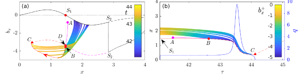
Figure 13 shows that the increase in downstream slope (that is, reduction in magnitude ) is key in ensuring that flux is not only reduced in the later stages of late drainage (as a flattening of already ensures), but actually vanishes entirely on reaching the boundary of the blank region of zero flux (marked in the equivalent figure 6): compare panels a–b of figure 13 with panel c, which shows the equivalent orbit for a lake that drains completely after the inital seal incision. Reaching that boundary in 13 implies that flow ceases abruptly, and the lake re-seals.
The case shown in figure 13(a) is additionally visualized in figure 14, where we show characteristics that reach the shock from downstream as multicoloured curves, the colouring indicating time (panel a) or slope along the characteristic (panel b). The increasingly rapid transit of characteristics past the point (vertical dotted line marked in panel a) and the reduced steepening at later times during lake drainage is evident in panels a (later characteristics do not dip to larger negative values of , and the colouring indicates only a short amount of time spent near ) and b (later characteristics are steeper near , indicating a faster passage, and retain a lighter blue colour indicating less steep slopes).
The effect of downstream flattening during seal incision becomes stronger if storage volume is large or the inflow is smaller (but still above the critical value for the initiation of drainage as discussed in section 4.2). Both larger or smaller lead to a bigger relative increase in flux during lake drainage, and hence to a stronger relative flattening of the downstream slope. This accounts for oscillatory drainage occurring at such parameter combinations in figure 10.
Spontaneous termination of lake drainage however need not lead to periodically recurring lake drainage, see for instance figure 8(d2) and 13(b): consecutive filling and drainage cycles may have an increasing amplitude, leading to complete lake emptying eventually. This appears to be linked to rapid re-filling of the lake and re-activation of the same shock that caused the initial incision. Once the reactivated shock incises the smooth seal again, it may do so with a steeper downstream slope and incise further upstream (figure 13(b)).
Reactivation of the same shock is favoured by small lake storage capacity and larger fluxes , which allow the lake to refill rapidly. As a result, the shock that originally incised the smooth seal is not advected far enough downstream, and on reactivation reaches the re-formed smooth seal again. Periodic lake drainage by contrast results most easily if is larger and inflow rates are small but above the critical value for drainage.
In that case, lake re-filling takes longer and the shock that incised the seal on the previous drainage cycle is advected far enough downstream between cycles for it not to return to incise the seal again. This is illustrated in figure 14. The ice surface rebuilds to a local steady state solution everywhere upstream of the advected shock by the time the lake refills and outflow of water recommences (the black curve in 14(a), with the advected shock being marked by ; the dashed black curve continues the steady state solution past the advected shock, where it now represents the unincised ice surface ). When flow of water recommences, a new channel is incised and a new shock is formed in this previously steady part of the ice surface (the pink red line originating at point A in 14(a), see also the pink line in figure 8(d)1). This new shock migrates upstream, intersecting the rebuilt smooth seal at point B in figure 14(a). Crucially, all characteristics that reach the new shock from downstream during the drainage cycle also originate upstream of the old shock (the coloured lines in figure 14(a), all of which start upstream of ). Once flow terminates again (point C), the new shock is in turn advected downstream, with a new smooth seal forming at point D. The new shock reaches the position of the previous shock at the start of the next cycle, which repeats the previous one exactly.
Importantly, we have observed oscillatory behaviour only for . For the examples we have computed with (figure 11), lake drainage is either complete or flux becomes infinite in finite time, with regularized solutions showing complete drainage even then (figure 9(a)). A closer examination reveals that, for the uplift rate and parameter values used in our calculations, the downstream slope does not actually decrease (become less negative) during lake drainage for (figure 15) unlike the case reported above.
This occurs because the shock that breaches the initially smooth lake seal forms at the seal location itself. As lake drainage proceeds, increases in flux do cause characteristics to migrate at a faster rate and therefore to experience less steepening as already described above. These characteristics however originate further downstream from the smooth lake seal, and therefore start with a steeper slope because the initial conditions dictate as much. The initially steeper slope dominates and downstream slopes continue to steepen at the backward-migrating shock until lake drainage is complete, see figure 15(a).
That is not to say that periodic drainage is impossible for , but we have not found any examples in which it occurs for the particular uplift function and initial conditions used here. We also reiterate that the flood termination mechanism described above involves a surface shape that flattens upstream of the seal, as is likely to be generically the case for surface lakes on ice sheets that form due to a smooth local uplift anomaly. Lakes whose bottom does not flatten out do occur on mountain glaciers, for instance at glacier confluences [63]. We investigate this situation in §5.2 of the supplementary material, prescribing an uplift velocity such that tends to a positive constant far upstream of the smooth lake seal (that is, the lake surface does not flatten). Repeated floods with constant lake supply are much less common, and follow a somewhat different mechanism: the same shock reactivates in each cycle but does not steepen from cycle to cycle in such a way as to cause complete lake drainage.
5 Discussion and Conclusions
In this paper, we have derived and solved a reduced, ‘stream power’-type model [50] for supraglacial stream incision (equations (10)), coupled to a model for lake drainage to determine the water flux (equations (12)), whose value depends on whether and how fast the stream is cutting into the lake seal. Note that, for completeness, the model is stated in dimensional form in §1 of the supplementary material. At the most basic level, the model predicts that a lake drains if water input to the lake is sufficiently large to overcome the effect of forward advection of the channel by the flow of the ice: if the inflow criterion (34) is satisfied (again stated in dimensional form in §1 of the supplementary material), then the incision of the outflow channel will cause the lake seal to be breached eventually by a backward-propagating shock. The criterion demonstrates that sufficiently large water supply, steep downward slopes on the far side of the seal (large , where is the uplift velocity of the ice) and slow advection (small values of the horizontal velocity ) is key to lake drainage. In particular, forward advection of the channel is the critical difference between the supraglacial lake drainage case and other dam burst phenomena [e.g. 64]. Qualitatively, our lake drainage criterion (34) is at least consistent with the observation [1] that non-draining lakes in Greenland are located at higher elevations (where water supply rates will be smaller, as are vertical velocities ) compared with ‘slowly draining lakes’, which may conceivably drain through surface channels rather than hydrofracture.
The model also predicts that initial incision into the seal need not lead to complete lake drainage. Instead, a flattening of both upstream and downstream slopes at the shock at the downstream end of the lake can lead to the lake re-sealing, with forward advection of the shock subsequently causing the original lake basin to re-form. The flattening of the downstream slope is facilitated not only by relatively slow water inflow rates to the lake but also, and perhaps counterintuitively, by a large lake storage capacity, with both facilitating a large relative increase in discharge during lake drainage and rapid retreat of the lake-terminating shock that ultimately causes the slopes downstream of the shock to flatten again (§4.3).
The dynamics of supraglacial lakes in our model ultimately permit four different outcomes: no incision of the seal (at inflow rates below the critical value given by condition (34)), a periodic cycle of the lake being breached and draining, followed by refilling (at large storage capacity and small above-critical water inflow), a sequence of lake drainage epsiodes of growing amplitude that progress until the lake fully empties (at intermediate storage volumes and water supply rates), and complete lake drainage at small storage volumes and large water supply rates. The possibility of oscillatory lake behaviour by overland drainage in particular has implications for the interpretation of lake observations by remote sensing, where the drainage mechanism may not be immediately apparent: in principle, it permits lakes to drain ‘unexpectedly’, that is not, not during the height of the melt season [e.g. 31, 28], and for lakes to remain filled for multiple melt seasons until the seal is breached again (see also §5.1 of the supplementary material). However, unlike the condition (34) for seal breaching, we are unable to give simple criteria for complete versus partial, oscillatory lake drainage; presumably, the boundaries between these phenomena in parameter space depends on the specifics of the uplift velocity .
One shortcoming of our model relevant to these different drainage styles is its one-dimensional nature. Implicit here is that, even if drainage terminates and the lake re-seals, subsequent overflowing of the reconstituted lake will re-activate the same channel as before. This is key to the drainage cycles with growing amplitude, leading to the lake emptying fully (column 2 of figure 8): the re-activation of the previous channel leads to subsequent drainage of the lake progressing further. If instead the previous channel is advected laterally as well as down-slope [48], then a new channel may be formed each time and periodic drainage cycles may in fact be more common than our results indicate.
More broadly, it is worth revisiting the construction of our model. The glacial case is perhaps the simplest in which a ‘stream power’ model for channel incision can be justified from first principles: the product of ‘erosion’ by flowing water is simply more water, rather than sediment whose transport must then be accounted for [61]. Our results however do indicate that the model as stated is incomplete: the predictions of the model depend strongly on the choice of the exponent that parameterizes the cross-sectional shape of the channel in our model (§2.1). For instance, for channels of fixed width (independently of their cross-sectional area) we have . Unlike the case of channels with variable width (), we have found no oscillatory lake drainage (§4.1 and §4.3) when . Instead, the lake can drain ‘abruptly’ in the sense that flux becomes large, incision becomes rapid and water level in the lake does not remain close to the height of the seal as stipulated by (12); in the model consisting of (10)–(12), this phenomenon manifests itself as flux becoming singular unless (12) is regularized (§3.4–4.1).
To determine even the qualitative behaviour of lake drainage unambiguously, a more sophisticated model for channel evolution is therefore necessarily, capable of predicting the shape of cross-sections self-consistently instead of imposing it as a constitutive relation. There is currently no particularly good template, though the work in Dallaston and Hewitt [55] may be a good starting point. Closely linked to cross-sectional shape evolution is the need to be able to predict meandering [57, 58], which ultimately should modify our large scale model (10) through the introduction of an evolving tortuosity. Not only is a model for cross-sectional shape now required, but the secondary flows involved in meandering instabilities also need to be accounted for, which also occur at wavelengths comparable to channel width [57]. (That being said, it is worth remembering that even the more sophisticated subglacial drainage models in existence [e.g. 65] do not attempt to account for evolving tortuosity.) Lastly, the ability to account not only for lateral instabilities driving meandering, but also for bedform formation and roll waves at supercritical Froude numbers [53, see also §3.2 of the supplementary material] is also desirable, in order to be able to apply the model on steeper slopes or at large discharge rates.
There are numerous other shortcomings to our model as described in §2.1, such as the neglect of melting due to heat exchange with the atmosphere and solar radiation, accumulation of snow in the channel, and exchange of water with an underground firn aquifer. We conclude by pointing out that, these issues notwithstanding, our model provides a template for improving previous surface drainage models due to Raymond and Nolan [35] and Kingslake et al. [38]. As with the prior, though slightly different work in Walder and Costa [34] (which considers the widening rather than deepening of a pre-existing breach through the full thickness of an ice dam), the models for downward incision of a channel in Raymond and Nolan [35] and Kingslake et al. [38] are heavily parameterized and do not resolve position along the channel. In effect, they are ad hoc versions of the boundary layer problem in our appendix B.2, aiming to compute the function of §3.4 here: Raymond and Nolan [35] equate the difference between lake level and seal height ( in appendix B.2) with the far field water depth in the same boundary layer (our in appendix B.2), while Kingslake et al. [38] questionably impose Bernouilli’s law (valid in the inertia-dominated upstream far field of the boundary layer) at the same time as a balance between the downslope force of gravity and friction at the channel wall (valid in the friction-dominated downstream far field). The details of those calculations aside, it is unclear whether the precise form of the relationship between flux and water height above the lake seal are key to modelling a supraglacial outburst flood: our work suggests that it may often (except in the flux singularity case for fixed width channels illustrated in figure 9(a1–c1)) suffice to require that lake level remains approximately at the seal, and to focus instead on the incision of the channel over longer length scales, which allows the channel slope at the shock-like lake seal to change as the outburst flood progresses, changing the rate of backward migration of the seal and hence the rate of lake drainage.
Appendix A Asymptotics of the ponded region
We assume as given by the dimensionless version of (1f); for more general forms of , see the supplementary material. The rescaling of (5) relevant to a ponded section of the channel becomes
| (35) |
We also assume : The mass storage term, in (5a), then does not appear at leading order in the leading order model and flux remains constant as assumed above in (10).
Specifically, at leading order, (5) becomes
| (36) |
Here is rescaled water depth. Equation (36)3 is indeed (10a) with ; the only issue is making sure that is correctly defined.
From (36)2, the surface elevation remains constant. The boundary layers of appendices B.2 and B.3 confirm that there is no leading order jump in at the end of a ponded section, and we have , at the ends of a ponded section in order to match to the flowing sections. Hence takes the same value at both ends of the ponded section, and (since ), is below that value inside the ponded section. Since we must have in any flowing section then, with , the ponded section must terminate at a local maximum of . The definition for the union of ponded sections follows as does the ponding function in equation (10).
Appendix B Boundary layers
A shock forms where the bed slope changes discontinuously in equation (10). In the full scaled model (5), that change in slope is not discontinuous but occurs over a short length scale . Assuming that the shock is at a moving location , the appropriate rescaling is
| (37) |
where is the outer solution satisfying (10), and the superscript ‘’ denotes the limit taken as is approached from below. We will likewise use the superscript ‘’ for the limit taken from above. At leading order we find that . Matching with the upstream far field, we deduce from (5a) that and , where .
We restrict ourselves to (1f) as constitutive relations here: the supplementary material shows that the qualitative boundary layer results are unchanged under relatively mild restrictions on wetted perimeter and water depth . With the constitutive relations (1f), the remainder of (5a) becomes, after some manipulation,
| (38a) | ||||
| (38b) | ||||
or, as a single equation
| (39) |
As we discuss further in section 2 of the supplementary material, we must assume both far field velocities to be subcritical in order for our leading order model to hold: denoting , subcriticality requires , and the right-hand side of (39) remains bounded.
There are different types of shocks to consider, each corresponding to different far-field conditions. We sketch each in turn.
B.1 The knickpoint boundary layer
For a shock connecting two flowing sections, and satisfy the far field equation (6)2, . must be distinct equilibria of (39), which requires
| (40) |
and as discussed in section 3.2 for shocks of this type. The solution then connects to as required provided is the stable equilbrium, and hence or (figure 16(a)). In common with the other boundary layers below, note also that the outer solution is continuous at as assumed in sections 3.2–3.3 and appendix C: represents only a small correction in channel base elevation (see again figure 16(a)).
B.2 The seal downstream of a ponded section
If the upstream far-field is ponded and satisfies (36), we have and as , and the bed slope is no longer related to through (6)2. The solution must again connect upstream to a finite downstream, satisfying once more. must again be subcritical, and an equlibrium of (39), which implies
| (41) |
as in equation (17) with . With , the fixed point is then guaranteed to be stable, and there is a solution connecting to . Note that a seal solution is possible even if (which is not the case for the shock solution of the previous section).
By matching with the upstream, ponded solution we can also show that surface elevation in the ponded section exceeds the seal height by an amount of , assuming that there is indeed flow with : this is done by integrating the water level correction defined by to with respect to as explained in further detail in the supplementary material. The finite value of justifies equating water level in the ponded region with the seal height at leading order as in appendix A. Moreover, since the boundary layer solution is fully determined by the model parameters and by far field forcing though , and , we can establish a functional relationship between the outer water level correction and , and as assumed in equations (25) and (26), where . An example is shown in figure 17(b).
Note that the boundary layer description above does not cover the case of a ‘smooth’ seal, where there is no shock. The corresponding reformulation of the boundary layer is based on the alternative rescaling
and assumes that . The boundary layer model can be rewritten as a modified version of (39)
| (42) |
where if , otherwise. We need to match as and as . For , such a solution always exists, while for , solutions only exist conditionally: if , we must have or , . Details may be found in §2.8 of the supplementary material.
B.3 Upstream end of a ponded section
A flowing section entering a ponded section can also be treated using the boundary layer model (39), with the upstream far field given by (6)2, and downstream. Such a solution requires that be an unstable fixed point, or equivalently
| (43) |
This is the case if either or , which also ensures that is a stable fixed point as required. These conditions on justify the analysis in appendix C below, and in particular justifies equation (48). We still obtain a relationship between the jump in slope and the migration rate, since
| (44) |
as , so as in equation (46) below.
Appendix C Entry into a ponded section in the outer model
We use appendix B.3 to determine conditions on the outer model (10) at the upstream end of a ponded section, where , . This situation never corresponds to a shock, but can give rise to an expansion fan. Characteristics upstream of the ponded section move more slowly, at , than those downstream of the transition to ponded, at . Consequently, characteristics must emerge from at least one side of the transition, whose location we denote by (figure 4(d)). The height is given by the seal at the (distant) downstream end of the ponded section, which controls the migration rate . Again differentiating both sides of and rearranging, is
| (45) |
If (so ), then characteristics emerge upstream and enter from downstream, with no jump in at Conversely, if (so ), then characteristics emerge downstream with no jump in . Upstream, characteristics enter the transition point, or are tangent to . In either case, the requirement that remain continuous (equation (17)) is now a jump condition for the slope ,
| (46) |
being given through (45): equation (46) is the same as (44).
The two cases identified above leave a third possibility where, instantaneously,
| (47) |
For and with given by (8), this range is non-void if and only if (or more generally, if is strictly convex in its first argument with ). Characteristics now have to emerge on both sides as an expansion fan, whose behaviour is non-trivial. The problem as stated is underdetermined, since the evolution of along the curve (and therefore itself beyond the initial instant) is undetermined in the absence of characteristics intersecting .
From (43), the migration rates implied by (47) cannot be sustained for finite time spans: the expansion fan must adjust so that does not remain in this forbidden range. From (45), cannot be attained by changing along the transition curve if . Hence must adjust to attain . In other words, the expansion fan upstream of must span all slopes between the initial and a less steep slope at which the motion of is locally parallel to a characteristic on which , determined implicitly through
| (48) |
Equivalently,
| (49) |
where , and are evaluated at slope . Characteristics on the upstream side of emerge tangentially to the transition curve , and the slope of characteristics emerging on the downstream side is then related to through (46).
Appendix D Numerical solution
We solve the problem consisting of (10) and (12) using the method of characteristics, appropriately modified to handle ponding and the outflow from the lake that determines . Given a set of values , we define as the point at which the straight lines and intersect, extrapolating from linearly from and . We put as the interpolant for that point. If there is a shock between points and , its location is at , and at the shock is to second order accuracy.
Let superscripts denote solutions at time . Assume a lake level and solution at discrete points is given, with the being ordered so that . For given and , let be the set of seal points downstream of , and let be an estimate for the highest point in the channel downstream of . Put if , otherwise. Let be the discrete seal point height for the lake, which is second order accurate regardless of whether the seal is at a shock or not. We update by a backward Euler step
| (50a) | |||
| Note that the lagged time variable indicates that we are using a fixed ponding function , computed from the last known solution. We use two methods of computing water level and flux . For , we use (12) as stated, | |||
| (50b) | |||
with and being prescribed functions. For , (50b) may not have a unique solution as described in section 3.4, and we replace (50b) with (25), in the form
| (51) |
We treat simply as a regularization rather than trying to emulate the function shown in figure 17(b), and consequently we drop the slopes and as arguments from . In practice, we use if , otherwise, and put . The system of equations (50) for the updated variables is solved using a semi-smooth Newton solver. Time step size is chosen so that no characteristic moves further than the spacing between adjacent characteristics in a single time step.
The updated solution is then post-processed for shocks, and to add characteristics where the points have become too widely spaced and account for expansion fans. Any characteristic with outside the domain is deleted, and the remainder is relabelled. Next, we compute the , , and , and identify any for which . For these , we assume there is a shock that the th characteristic has crossed, and delete the th characteristic from that time forward, and relabel the remaining characteristics. Likewise if , we delete the th characteristic, repeating the entire postprocessing step (including computation of and ) until there are no intervals left such that lies outside that interval. This also ensures the remaining points are ordered.
If subsequently any are above a prescribed tolerance, we introduce new characteristics between them at a prescribed spacing. If and , we construct a piecewise linear interpolation between and with constant slope below and above a pond entry position (itself solved for as part of the construction of the interpolation) chosen such that , and such that the discontinuity in slope at satisfies (46)–(45). Otherwise, we construct a linear interpolant between and to initialize the new characteristics, provided the characteristics are indeed spreading with . If the characteristics are not spreading, new points are introduced by extrapolation from for any new points with , and from otherwise.
References
- Poinar and Andrews [2021] K. Poinar and L.C. Andrews. Challenges in predicting Greenland supraglacial lake drainages at the regional scale. The Cryosphere, 15:1455–1483, 2021. doi: 10.5194/tc-15-1455-2021. URL https:/doi.org//10.5194/tc-15-1455-2021.
- Lenaerts et al. [2016] J.T.M. Lenaerts, S. Lhermitte, S.R.M. Drews, R.and Ligtenberg, Berger S., Helm V., C.J.P.P. Smeets, M.R. van den Broeke, W.J. van de Berg, W. van Meijgaard, M. Eijkelboom, O. Eisen, and F. Pattyn. Meltwater produced by wind-albedo interaction stored in an East Antarctic ice shelf. Nature Geoscience, 7:58–62, 2016. doi: 110.1038/NCLIMATE3180. URL https://doi.org/10.1038/NCLIMATE3180.
- Kingslake et al. [2017] J. Kingslake, J. Ely, I. Das, and R. Bell. Widespread movement of meltwater onto and across Antarctic ice shelves. Nature, 544:349–352, 2017.
- Stokes et al. [2019] C.R. Stokes, J.E. Sanderson, S.S.R. Miles, B.W.J.and Jamieson, and A.A. Leeson. Widespread distribution of supraglacial lakes around the margin of the East Antarctic Ice Sheet. Scientific Reports, 9:13823, 2019. doi: 10.1038/s41598-019-50343-5. URL https://doi.org/10.1038/s41598-019-50343-5.
- Das et al. [2008] S.B. Das, I. Joughin, M.D. Behn, I.M. Howat, M.A. King, D. Lizarralde, and M.P. Bhatia. Fracture Propagation to the Base of the Greenland Ice Sheet During Supraglacial Lake Drainage. Science, 320:778–781, 2008.
- Cowton et al. [2013] T. Cowton, P. Nienow, A. Sole, J. Wadham, G. Lis, I. Bartholomew, D. Mair, and D. Chandler. Evolution of drainage system morphology at a land-terminating Greenlandic outlet glacier. J. Geophys. Res. Earth Surf., 118:1–13, 2013. doi: 10.1029/2012JF002540. URL https://doi.org/10.1029/2012JF002540.
- Chandler et al. [2013] D.M. Chandler, J. Wadham, G. Lis, T. Cowton, A. Sole, I. Bartholomew, J. Telling, E.B. Nienow, P.and Bagshaw, D Mair, S. Vinen, and A. Hubbard. Evolution of the subglacial drainage system beneath the Greenland Ice Sheet revealed by tracers. Nature Geoscience, 6:195–198, 2013. doi: 10.1038/NGEO1737. URL https://doi.org/10.1038/NGEO1737.
- Shepherd et al. [2009] A. Shepherd, A. Hubbard, P. Nienow, M. King, M. MacMillan, and I. Joughin. Greenland ice sheet motion coupled with daily melting in late summer. Geophys. Res. Lett., 36(L01501):doi:10.1029/2008GL035785, 2009.
- Schoof [2010] C. Schoof. Ice-sheet acceleration driven by melt supply variability. Nature, 468:803–806, 2010.
- Palmer et al. [2011] S. Palmer, A. Shepherd, P. Nienow, and I. Joughin. Seasonal speedup of the Greenland Ice Sheet linked to routing of surface water. Earth and Planetary Science Letters, 302(3-4):423–428, 2011.
- Tedesco et al. [2013] M. Tedesco, I.C. Willis, M.J. Hoffman, A.F. Banwell, P. Alexander, and N.S. Arnold. Ice dynamic response to two modes of surface lake drainage on the Greenland ice sheet. Env. Res. Lett., 8:034007, 2013. doi: 10.1088/1748-9326/8/3/034007. URL https://doi.org/10.1088/1748-9326/8/3/034007.
- Lüthje et al. [2006] M. Lüthje, L.T. Pedersen, and W. Reeh, N.and Greuell. Modelling the evolution of supraglacial lakes on the West Greenland ice-sheet margin. J. Glaciol., 52(179):608–617, 2006. doi: 10.3189/172756506781828386. URL https://doi.org/10.3189/172756506781828386.
- Tedesco et al. [2012] M. Tedesco, M. Lüthje, K. Steffen, N. Steiner, X. Fettweis, I. Willis, and N. Bayou. Measurement and modeling of ablation of the bottom of supraglacial lakes in western Greenland. Geophys. Res. Lett., 39:L02502, 2012. doi: 10.1029/2011GL049882. URL https://doi.org/10.1029/2011GL049882.
- Scambos et al. [2004] T.A. Scambos, J.A. Bohlander, C.A. Shuman, and P. Skvarca. Glacier acceleration and thinning after ice shelf collapse in the Larsen B embayment. Geophys. Res. Lett., 31(18):L18402, doi:1029/2004GL020670, 2004.
- Scambos et al. [2009] T. Scambos, H.A. Fricker, C.-C. Liu, J. Bohlander, J.and fastook, A. Sargent, R. Massom, and A.-M. Wu. Ice shelf disintegration by plate bending and hydro-fracture: Satellite observations and model results of the 2008 wilkins ice shelf break-ups. Earth and Planetary Sciience Letters, 280(1):51–60, 2009. doi: 10.1016/j.epsl.2008.12.027. URL https://www.sciencedirect.com/science/article/pii/S0012821X08007887.
- Banwell et al. [2013] A.F. Banwell, D.R. MacAyeal, and O.V. Sergienko. Breakup of the Larsen B Ice Shelf triggered by chain reaction drainage of supraglacial lakes. Geophys. Res. Lett., 40:5872–5876, 2013. doi: 10.1002/2013GL057694. URL https://doi.org/10.1002/2013GL057694.
- Lai et al. [2021] C.-Y. Lai, J. Kingslake, M.G. Wearing, P.-H. Cameron Chen, P. Gentine, J.J. Li, H.and Spergel, and J.M. van Wessem. Vulnerability of Antarctica’s ice shelves to meltwater-driven fracture. Nature, 584:574–578, 2021. doi: 10.1038/s41586-020-2627-8. URL https://doi.org/10.1038/s41586-020-2627-8.
- Straneo et al. [2011] F. Straneo, R.G. Curry, D.A. Sutherland, D.S. Hamilton, C. Cenedese, and L. Våge, K.and Stearns. Impact of fjord dynamics and glacial runoff on the circulation near Helheim Glacier. Nature Geoscience, 4:322–327, 2011. doi: 10.1038/NGEO1109. URL https://doi.org/10.1038/NGEO1109.
- Mortensen et al. [2020] J. Mortensen, S. Rysgaard, J. Bendtsen, K. Lennert, T. Kanzow, H. Lund, and L. Meire. Subglacial discharge and its down‐fjord transformation in west greenland fjords with an ice mélange. J. Geophys. Res. Oceans, 125:e2020JC016301., 2020. doi: 10.1029/2020JC016301. URL https://doi.org/10.1029/2020JC016301.
- Dallaston et al. [2015] M.C. Dallaston, I.J. Hewitt, and A.J. Wells. Channelization of plumes beneath ice shelves. J. Fluid Mech., 785:109–134, 2015. doi: doi:10.1017/jfm.2015.609.
- Washam et al. [2019] P. Washam, K.W. Nicholls, A. Münchow, and L. Padman. Summer surface melt thins Petermann Gletscher Ice Shelf by enhancing channelized basal melt. J. Glaciol., 65(252):662–674, 2019. doi: 10.1017/jog.2019.43.
- van der Veen [2007] C.J.. van der Veen. Fracture propagation as means of rapidly transferring surface meltwater to the base of glaciers. Geophys. Res. Lett., 34:L01501, 2007. doi: 10.1029/2006GL028385. URL https://doi.org/10.1029/2006GL028385.
- Stevens et al. [2015] L.A. Stevens, M.D. Behn, J.J. McGuire, S.B. Das, I. Joughin, T. Herring, D.E. Shean, and M.A. King. Greenland supraglacial lake drainages triggered by hydrologically induced basal slip. Nature, 522:73–76, 2015. doi: 10.1038/nature14480. URL https://doi.org/10.1038/nature14480.
- Christoffersen et al. [2018] P. Christoffersen, M. Bougamont, A. Hubbard, S.H. DOyle, S. Grigsby, and R. Pettersson. Cascading lake drainage on the Greenland Ice Sheet triggered by tensile shock and fracture. Nature Comms., 9:1064, 2018. doi: 10.1038/s41467-018-03420-8. URL https://doi.org/10.1038/s41467-018-03420-810.1029/2011GL049882.
- Koenig et al. [2015] L.S. Koenig, L.N. Lampkin, D.J.and Montgomery, S.L. Hamilton, J.B. Turrin, C.A. Joseph, S.E. Mousgafa, B. Panzer, J.D. Casey, K.A.and Paden, C. Leuschen, and P. Gogineni. Wintertime storage of water in buried supraglacial lakes across the Greenland Ice Sheet. The Cryosphere, 9:1333–1343, 2015. doi: 10.5194/tc-9-1333-2015. URL www.the-cryosphere.net/9/1333/2015/.
- Lampkin et al. [2020] K. Lampkin, D.J.and Koenig, C. Joseph, and J.E. Box. Investigating controls on the formation and distribution of wintertime storage of water in supraglacial lakes. Front. Earth Sci., 8:370, 2020. doi: 10.3389/feart.2020.00370. URL https://doi.org/10.3389/feart.2020.00370.
- Law et al. [2020] R. Law, N. Arnold, C. Benedek, A. Tedesco, M.and Banwell, and I. Willis. Over-winter persistence of supraglacial lakes on the Greenland Ice. J. Glaciol., 86(257):362–572, 2020. doi: 10.1017/jog.2020.7. URL https://doi.org/10.1017/jog.2020.7.
- Benedek and Willis [2021] C.L. Benedek and I.C. Willis. Winter drainage of surface lakes on the greenland ice sheet from sentinel-1 sar imagery. The Cryosphere, 15:1587–1606, 2021. doi: 10.5194/tc-15-1587-2021. URL https://doi.org/10.5194/tc-15-1587-2021.
- Dunmire et al. [2021] D. Dunmire, A.F. Banwell, N. Wever, J.T.M. Lenaerts, and R. Tri Datta. Contrasting regional variability of buried meltwater extent over 2 years across the Greenland Ice Sheet. The Cryosphere, 15:2983–3005, 2021. doi: 10.5194/tc-15-2983-2021. URL https://doi.org/10.5194/tc-15-2983-2021.
- Bell et al. [2018] R.E. Bell, A.F. Banwell, L.D. Trusel, and J. Kingslake. Antarctic surface hydrology and impacts on ice-sheet mass balance. Nature Clim. Change, 8:1044–1052, 2018. doi: 10.1038/s41558-018-0326-3. URL https://doi.org/10.1038/s41558-018-0326-3.
- Schaap et al. [2020] T. Schaap, M.J. Roach, L. Peters, S. Cook, B. Kulessa, and C. Schoof. Englacial drainage structures in an east antarctic outlet glacier. J. Glaciol., 66(225):166–174, 2020. doi: 10.5194/tc-14-3175-2020. URL https://doi.org/10.1017/jog.2019.92.
- Forster et al. [2013] R.R. Forster, J.E. Box, M.R. van den Broeke, C. Miège, E.W. Brugess, J.H. van Angelen, L.S. Lenaerts, J.T.M.and Koenig, J. Paden, C. Lewis, S.P. Gogineni, C. Leuschen, and J.R. McConell. Extensive liquid meltwater storage in firn within the Greenland ice sheet. Nature Geoscience, 7:95–98, 2013. doi: 10.1038/NGEO2043. URL https://doi.org/10.1038/NGEO2043.
- Meyer and Hewitt [2017] C. R. Meyer and I. J. Hewitt. A continuum model for meltwater flow through compacting snow. The Cryosphere, 11(6):2799–2813, 2017. doi: 10.5194/tc-11-2799-2017. URL https://tc.copernicus.org/articles/11/2799/2017/.
- Walder and Costa [1996] J.S. Walder and J.E.. Costa. Outburst floods from glacier-dammed lakes: the effect of mode of lake drainage on flood magnitude. Earth Surf. Proc. Landforms, 21:701–723, 1996.
- Raymond and Nolan [2000] C.F. Raymond and M.. Nolan. Drainage of a glacial lake through an ice spillway. In Symposium at Seattle — Debris-Covered Glaciers, volume 264 of IAHS Publications, pages 199–206. International Association of Hydrological Sciences, Wallingford, 2000.
- Mayer and Schuler [2005] C. Mayer and T.V. Schuler. Breaching of an icedam at Qorlortossup tasia, south Greenland. Ann. Glaciol., 42:297–302, 2005. doi: 10.3189/172756405781812989. URL https://doi.org/10.3189/172756405781812989.
- Vincent et al. [2010] C. Vincent, E. Auclair, and E. Le Meur. Outburst flood hazard for glacier-dammed Lac de Rochemelon, France. J. Glaciol., 56(195):91–100, 2010. doi: 10.3189/002214310791190857. URL https://doi.org/10.3189/002214310791190857.
- Kingslake et al. [2015] J. Kingslake, F. Ng, and A. Sole. Modelling channelized surface drainage of supraglacial lakes. J. Glaciol., 61(225):185–199, 2015.
- Ancey et al. [2019] C. Ancey, E. Bardou, M. Funk, M. Huss, M.A. Werder, and T. Trewhela. Hydraulic reconstruction of the 1818 Giéttro glacial lake outburst flood. Water Resources Research, 55:8840–8863, 2019. doi: 10.1029/2019WR025274. URL https://doi.org/10.1029/2019WR025274.
- Nye [1976] J.F. Nye. Water flow in glaciers: jökulhlaups, tunnels and veins. J. Glaciol., 17(76):181–207, 1976.
- Spring and Hutter [1981] U. Spring and K. Hutter. Numerical studies of jökulhlaups. Cold Reg. Sci. Tech., 4(3):227–240, 1981.
- Clarke [1982] G.K.C. Clarke. Glacier outburst floods from “Hazard Lake”, Yukon Territory, and the problem of flood magnitude prediction. J. Glaciol., 28(98):3–21, 1982.
- Ng [2000] F.S.L. Ng. Canals under sediment-based ice sheets. Ann. Glaciol., 30:146–152, 2000.
- Kingslake and Ng [2013] J. Kingslake and F. Ng. Modelling the coupling of flood discharge with glacier flow during jokulhlaups. Ann. Glaciol., 54(63):25–31, 2013.
- Stubblefield et al. [2019] A.G. Stubblefield, T.C. Creyts, J. Kingslake, and M. Spiegelman. Modelling oscillations in connected glacial lakes. J. Glaciol., 65(253):745–758, 2019. doi: 10.1017/jog.2019.46. URL https://doi.org/10.1017/jog.2019.46.
- Schoof [2020] C. Schoof. An analysis of instabilities and limit cycles in glacier-dammed reservoirs. The Cryosphere, 14:3175–3194, 2020. doi: 10.5194/tc-14-3175-2020. URL https://doi.org/10.5194/tc-14-3175-2020.
- Schoof [2002] C. Schoof. Basal perturbations under ice streams: form drag and surface expression. J.Glaciol., 48(162):407–416, 2002.
- Darnell et al. [2013] K.N. Darnell, J.M. Amundson, L.M. Cathles, and D.R. MacAyeal. The morphology of supraglacial lake ogives. J. Glaciol., 59(215):533–544, 2013. doi: 10.3189/2013JoG12J098. URL https://doi.org/10.3189/2013JoG12J098.
- Luke [1972] J.C. Luke. Mathematical models for landform evolution. J. Geophys. Res., 77(14):2460–24640, 1972.
- Whipple and Tucker [1999] K.X. Whipple and G.E. Tucker. Dynamics of the stream-power river incision model: Implications for height limits of mountain ranges,landscape response timescales, and research needs. J. Geophys. Res., 104:B8, 1999.
- Royden and Perron [2007] L. Royden and J.T. Perron. Solutions of the stream power equation and application to the evolution of river longitudinal profiles. J. Geophys. Res: Earth Surf., 118:497–518, 2007. doi: 10.1002/jgrf.20031. URL https://doi.org/10.1002/jgrf.20031.
- Kwang and Parker [2017] J.S. Kwang and G. Parker. Landscape evolution models using the stream power incision model show unrealistic behavior when equals 0.5. Earth Surf. Dynam., 5:807–1606, 2017. doi: 10.5194/esurf-5-807-2017. URL https://doi.org/10.5194/esurf-5-807-2017.
- Fowler [2011] A.C. Fowler. Mathematical geoscience, volume 36 of Interdisciplinary Applied Mathematics. Springer-Verlag, Berlin, 2011.
- Evatt et al. [2006] G. W. Evatt, A. C. Fowler, C. D. Clark, and N. R. J. Hulton. Subglacial floods beneath ice sheets. Phil. Trans. R. Soc. A, 364:1769–1794, 2006.
- Dallaston and Hewitt [2014] M.C. Dallaston and I.J. Hewitt. Free-boundary models of a meltwater conduit. Phys. Fluids, 26(8):0831011–22, 2014.
- Jarosch and Gudmundsson [2012] A.H. Jarosch and M.T. Gudmundsson. A numerical model for meltwater channel evolution in glaciers. The Cryosphere, 6(98):493–503, 2012. doi: 10.5194/tc-6-493-2012. URL www.the-cryosphere.net/6/493/2012/.
- Karlstrom et al. [2013] L. Karlstrom, P. Gajjar, and M. Manga. Meander formation in supraglacial streams. J. Geophys. Res.Earth Surf., 118:1897–1907, 2013. doi: 10.1002/jgrf.20135. URL https://doi.org/10.1002/jgrf.20135.
- Fernández and Parker [2021] R. Fernández and G. Parker. Laboratory observations on meltwater meandering rivulets on ice. Earth Surf. Dynam., 9:253–269, 2021. doi: 10.5194/esurf-9-253-2021. URL https://doi.org/10.5194/esurf-9-253-2021.
- Buzzard et al. [2018] S.C. Buzzard, D.L. Feltham, and D. Flocco. A mathematical model of melt lake development on an ice shelf. Journal of Advances in Modelling Earth Systems, 10:262–283, 2018. doi: 10.1002/2017MS001155. URL https://doi.org/10.3189/172756506781828386.
- Holmes [1995] M.H. Holmes. Introduction to Perturbation Methods, volume 20 of Texts in Applied Mathematics. Springer-Verlag, New York, 1995.
- Fowler et al. [2007] A.C. Fowler, N. Kopteva, and C. Oakley. The formation of river channels. SIAM J Appl. Math, 67(4):1016–1040, 2007. doi: 10.1137/050629264. URL https://doi.org/10.1137/050629264.
- Courant and Hilbert. [1989] R. Courant and Hilbert., editors. Methods of Mathematical Physics, volume 2. John Wiley & Sons, 1989.
- Werder et al. [2009] M.A. Werder, A. Loye, and M. Funk. Dye tracing a jökulhlaup: I. subglacial water transit speed and water-storage mechanism. J. Glaciol., 55(193):889–898, 2009. doi: 10.3189/002214309790152447. URL https://doi.org/10.3189/002214309790152447.
- Balmforth et al. [2009] N. Balmforth, J. von Hardenberg, and R.J. Zammett. Dam-beaking seiches. J. Fluid Mech., 628:1–21, 2009. doi: 10.1017/S0022112009005825. URL https://doi.org/10.1017/S0022112009005825.
- Werder et al. [2013] M.A. Werder, I.J. Hewitt, C.G. Schoof, and G.E. Flowers. Modeling channelized and distributed subglacial drainage in two dimensions. J. Geophys. Res., F118(4):2140–215, doi: 10.1002/jgrf.20146, 2013.