The distances to molecular clouds in the fourth Galactic quadrant
Abstract
Distance measurements to molecular clouds are essential and important. We present directly measured distances to 169 molecular clouds in the fourth quadrant of the Milky Way. Based on the near-infrared photometry from the Two Micron All Sky Survey and the Vista Variables in the Via Lactea Survey, we select red clump stars in the overlapping directions of the individual molecular clouds and infer the bin averaged extinction values and distances to these stars. We track the extinction versus distance profiles of the sightlines toward the clouds and fit them with Gaussian dust distribution models to find the distances to the clouds. We have obtained distances to 169 molecular clouds selected from Rice et al. The clouds range in distances between 2 and 11 kpc from the Sun. The typical internal uncertainties in the distances are less than 5 per cent and the systematic uncertainty is about 7 per cent. The catalogue presented in this work is one of the largest homogeneous catalogues of distant molecular clouds with the direct measurement of distances. Based on the catalogue, we have tested different spiral arm models from the literature.
keywords:
dust, extinction – ISM: clouds – Galaxy: structure1 Introduction
Distance is the fundamental parameter to estimate all other physical properties like the size and mass of molecular cloud. Estimating the distance to molecular cloud is a tough task and astronomers have explored several different techniques.
A first method is to derive the distance kinematically, which convert the radial velocity of a cloud to a distance by assuming that the cloud follows the Galactic rotation curve (e.g., Roman-Duval et al. 2009; Miville-Deschênes et al. 2017). However, the kinematic distances are problematic due to the large uncertainty of the rotation curve and the influence of the peculiar velocities and the noncircular motions. Furthermore, a well-known geometric ambiguity exists for the kinematic distance of cloud in the inner Galaxy, where one velocity can be related to two distances. A second method is to obtain the distance of a given cloud by identifying its associated objects having the same distance as the cloud, such as the OB stars and young stellar objects, whose distances can be estimated (e.g. Gregorio-Hetem 2008). However, this method is only applied to individual clouds of interest. A third method is to estimate the distance from the extinction of starlight, i.e., the extinction distance. As the density of the dust grains in the molecular cloud is much higher than that in diffuse medium, one can expect a sharp increase of stellar extinction at the location of the cloud. Thus the distance to the cloud can be obtained by finding the position where the extinction increases sharply.
The extinction method is directly measured and robust. However, it relies on the accurate estimates of distances and extinction values of a large number of stars. Thanks to a number of large-scale astrometric, photometric and spectroscopic surveys, we can obtain accurate values of distance and dust extinction for tens of millions of individual stars (e.g., Chen et al. 2014; Green et al. 2015). Thus the estimation of precise extinction distances to large samples of molecular clouds has become possible. Schlafly et al. (2014) obtain distances to dozens of molecular clouds selected from the literature by the three-dimensional (3D) extinction mapping method based on PanSTARRS-1 data. Zucker et al. (2019) improve their work by combining the optical and near-IR photometry with the Gaia Data Release 2 (Gaia DR2; Gaia Collaboration et al. 2018) parallaxes (Lindegren et al., 2018). Yan et al. (2019) derive extinction distances to 11 molecular clouds in the third Galactic quadrant. Chen et al. (2020) present accurate distance determinations to a catalogue of 567 molecular clouds based on estimates of colour excesses and distances of stars presented in Chen et al. (2019b). Zhao et al. (2018, 2020) estimate the extinction distances to 33 supernova remnants with the help of their association with molecular clouds.
All the above works calculate only the extinction distances to the nearby molecular clouds locating within 4 kpc from the Sun. These works are based on the optical extinction which becomes very large at far distances and they adopt the trigonometric parallax, photometric or spectroscopic distances of stars that suffer large uncertainties at far distances. Thus they are not able to determine the distances to far clouds. At far distances, the standard candle red clump star (RC) serves as a good tracers to infer the extinction distances of molecular clouds. RCs have almost constant luminosity and color. They are bright in the near-infrared (IR) bands and can trace the extinction profile at far distances (Gao et al., 2009; Güver et al., 2010; Gonzalez et al., 2012). Shan et al. (2018, 2019) use RCs to map the 3D extinction distribution of the sightlines toward the supernova remnants in the first and fourth quadrants of the Galaxy and estimate distances of them with extinction values from the literature. Wang et al. (2020) use RCs to estimate extinction distances of 63 molecular clouds and infer them to the distances of supernova remnants.
In this work, we select RCs from the near-IR colour-magnitude diagram (CMD) to determine the distance to a large sample of molecular clouds in the fourth Galactic quadrant based on the data from the Two Micron All Sky Survey (2MASS; Skrutskie et al. 2006) and the Vista Variables in the Via Lactea Survey (VVV; Minniti et al. 2010). We select molecular clouds from Rice et al. (2016), who present a catalogue of 1,064 massive molecular clouds throughout the Galactic plane from the CO survey of Dame et al. (2001). We have estimated robust, directly-measured distances of 169 molecular clouds. The most distant cloud is located at a distance larger than 11.5 kpc from the Sun.
The paper is structured as follows. In Section 2, we describe the data. In Section 3 we introduce our method for determining the distances to the molecular clouds. We present our results in Section 4, and discuss them in Section 5. We summarize in Section 6.
2 Data

Our work is based on near-IR photometry from 2MASS and VVV. 2MASS was conducted with two 1.3 m telescopes to provide full coverage of the sky. It has three near-IR bands, and , centred at 1.25, 1.65, and 2.16 m, respectively. The 2MASS Point Source Catalog (PSC; Skrutskie et al. 2006) contains near-IR photometry for over 500 million objects. The systematic uncertainties of 2MASS photometric measurements are estimated to be smaller than 0.03 mag. The 10 limiting magnitude is approximately 14.3 mag. To trace the distance of far molecular clouds, we combined the 2MASS data with the in-depth near-IR VVV data. The VVV survey were carried out with the VISTA 4.1 m telescope. The survey took images in five bands, and . The total survey area of VVV is 560 deg2, including a region of the Galactic plane of 295° 350° to 2°2°and the Bulge of 10°10° and 10° 5°. In the current work, we adopt the catalogue ‘vvvPsfDophotZYJHKsSource’ from the Data Release 4 of Images and Source Lists from VVV111https://www.eso.org/sci/publications/announcements/sciann17009.html. The VVV saturation limit ranges between 10 – 12 mag, and the photometric limit is typically 17.5 mag (Saito et al., 2012).
In this work, the molecular clouds are selected from the work of Rice et al. (2016), who have created a catalogue of massive molecular clouds in the Galactic plane (13° 348°) with a consistent dendrogram-based decomposition of the CO data from the 12CO CfA-Chile survey (Dame et al., 2001). The Rice et al. catalogue contains 1,064 massive clouds. 247 of them are located inside the VVV survey footprint. All of them are located in the fourth quadrant of the Galactic plane.
For each molecular cloud, we select stars from the 2MASS and VVV catalogues in a square that centres at the the cloud with a side length of its size (), i.e. and , where and are the Galactic coordinates of the cloud centre. We require that the stars must have detections in both the and bands and have uncertainties in the two bands smaller than 0.1 mag. To combine the 2MASS and VVV data, we first convert the VVV magnitudes to the 2MASS ones with the transformation equations from Soto et al. (2013). The transform equations from Soto et al. (2013) are derived from de-reddened magnitudes and colours of stars. In this work we have ignored the effects of the variation of transformation coefficients caused by the dust extinction. The impacts on the transformed magnitudes and colours are likely to be small. For example, a disk RC that suffers an extinction value of = 1 mag, will result in uncertainty in the colour of about 0.06 mag. Then we merge the 2MASS and VVV data by using the 2MASS data for 12.5 mag, and the VVV data for 12.5 mag. For some of the molecular clouds, there are only a few stars located in the defined boxes due to their small sizes. We exclude the clouds that contain less than 5,000 stars. It yields 230 clouds in our sample. Fig. 1 shows the spatial distribution of these molecular clouds. In the left panel of Fig. 2, we show the (, ) CMD of an example cloud. There are 108 973 stars, with 3 700 and 105 273 stars from 2MASS ( 12.5 mag) and VVV ( 12.5 mag), respectively.
3 Method

To obtain the extinction and distance profile of the sightline toward a given molecular cloud using the RCs, we first determine an empirical track of RCs by linking all peaks of the colour histograms of the RC candidates in the individual magnitude bins from the (, ) CMD. Similar to the previous works (e.g., Gao et al. 2009 and Wang et al. 2020), we check the CMD by naked eyes to achieve a rough stripe of RCs. The borders of the RC candidates are defined as two cubic polynomial function that fit seven points manually selected. We then select stars inside the boundaries and divide them into different horizontal bins according to their magnitude. As the stellar densities differ from different magnitude, we choose every 25 stars a bin for 10 mag and every 0.1 mag a bin for 10 mag. For each bin, we fit the distribution of the stellar colours with a Gaussian function to obtain its peak colour and the corresponding width. In the left panel of Fig. 2, we show an example of how the RC track is defined. Due to the completeness limit of the observing data, the RC track moves to leftward for those faintest magnitude bins. We manually define a cutoff magnitude for each cloud to avoid the effect.
The resultant RC track is then used to measure the extinction profile of the sightline of the cloud. As RCs have almost a constant intrinsic color and absolute magnitude, we can easily convert their colours and magnitudes (, ) into distances and extinction values (, ) by,
| (1) |
and
| (2) |
where we adopt the extinction coefficient of 0.473 from Wang & Chen (2019), the intrinsic color of RC = 0.7 mag from Grocholski & Sarajedini (2002) and the absolute magnitude of RC = 1.61 mag (Alves, 2000).
We finally determine the distance of a cloud based on the extinction profile of the cloud sightline. We fit the extinction profile within the distance range of the cloud by,
| (3) |
where is the -band extinction contributed by the diffuse medium and contributed by the dust within the molecular cloud at distance . For the diffuse component, we have tested different models, such as the fourth-order polynomial (Chen et al., 1998), the quadratic polynomial (Chen et al. 2017a, Yu et al. 2019, and Zhao et al. 2020), linear polynomial (Marshall et al., 2009), and constant (Schlafly et al. 2014 and Chen et al. 2020), and decide to adopt the linear polynomial, as,
| (4) |
where and are polynomial coefficients. Assuming a simple Gaussian distribution of dust in the cloud (Chen et al. 2017a, Yu et al. 2019, and Zhao et al. 2020), the extinction profile of the cloud is then given by,
| (5) |
where is the width of the extinction jump, is the total extinction contributed by the dust grains in the cloud and is the distance of the cloud.
For each cloud, the polynomial coefficients and , the total extinction , and the distance of the cloud are free parameters to fit. It is difficult for us to constrain the width of the extinction jump in our model since there is significant degeneracy between and . We tried to fit with several different priors, but those fits failed for a large number of clouds. Finally we decide to adopt a fixed for each cloud. As discussed by Chen et al. (2020), for distant clouds, the widths of the extinction jumps are mainly dominated by the distance uncertainties of the extinction profile. In the current work, we assume the width of the extinction jump of each cloud consists of two components, the size of the cloud and the distance uncertainty, i.e., , where is the size of the cloud (), and is the uncertainty of the distance. The typical distance uncertainty of RC is 7 per cent (see Sect. 5.1). We thus adopt . This assumption works well for our model, and we are able to successfully fit most of the extinction jumps.
A simple Bayesian scheme is adopted to obtain the free parameters and their statistical uncertainties. We adopt the likelihood
| (6) |
where and are the -band extinction profile derived from the RC track and that modeled by Equation (2)–(4).
For the distance , we adopt a prior based on the kinematic distance of the cloud by,
| (7) |
which means that we are only looking for the molecular clouds around its kinematic distance within 50 per cent of its kinematic distance or 1.5 kpc if the 50 per cent kinematic distance is too small. If there are near-far distance ambiguity, we search for the cloud around both the near and far kinematic distances. Since the Rice et al. (2016) catalogue provides only one kinematic distance value for each cloud, either the near of the far ones, we calculated the kinematic distances of all the selected clouds by the same algorithm as Rice et al. (2016) but with Galactic and Solar parameters from Reid et al. (2019). Our derived kinematic distances are almost the same as those from Rice et al. (2016). If there is no kinematic distance resulted from the algorithm, we adopt a flat prior for all distances. For other parameters, we adopt flat priors,
| (8) |
The MCMC algorithm emcee (Foreman-Mackey et al., 2013) is applied in the current work. The resulting distance and its statistical uncertainty are estimated in terms of the 50th, 16th and 84th percentile of the distance samples from the MCMC chain. In the right panel of Fig. 2, we show an example of how the extinction profile is fitted.
4 Results


| () | () | () | (kpc) | (mag) | (pc) | (103 M⊙) | () | (kpc) |
|---|---|---|---|---|---|---|---|---|
| 296.10 | 0.22 | 0.20 | 5.290.69 | 0.11 | 35 | 39.42 | 13.47 | 8.40 |
| 297.83 | 0.70 | 0.42 | 3.350.31 | 0.12 | 46 | 190.70 | 33.46 | 3.89 |
| 298.89 | 0.43 | 0.28 | 3.260.33 | 0.11 | 30 | 98.52 | 37.98 | 4.03 |
| 298.93 | 0.16 | 0.12 | 8.661.22 | 0.14 | 34 | 88.78 | 19.39 | 6.17 |
| 299.27 | 0.18 | 0.09 | 8.590.62 | 0.30 | 25 | 47.44 | 11.32 | 9.01 |
| 301.38 | 0.27 | 0.12 | 5.860.85 | 0.13 | 23 | 65.34 | 38.46 | 4.34 |
| 301.75 | 0.92 | 0.39 | 3.960.37 | 0.15 | 51 | 389.25 | 41.00 | 4.39 |
| 301.79 | 0.01 | 0.15 | 5.860.68 | 0.13 | 29 | 57.10 | 23.71 | 10.57 |
| 303.04 | 0.47 | 0.53 | 6.150.48 | 0.19 | 108 | 1325.45 | 33.02 | 3.31 |
| 303.44 | 1.67 | 0.11 | 3.610.32 | 0.33 | 13 | 37.60 | ||
| 304.04 | 1.02 | 0.13 | 3.910.39 | 0.19 | 16 | 45.84 | 35.96 | 3.56 |
| 304.16 | 1.43 | 0.18 | 4.460.57 | 0.12 | 26 | 33.00 | 45.09 | 4.68 |
The Table is available in its entirety in machine-readable form
in the online version of this manuscript and also at the website
“http://paperdata.china-vo.org/diskec/rjcloud/table1.dat”.
We have applied the distance estimation algorithm to all the selected 230 giant molecular clouds. Similar as in the example shown in Fig. 2, we can clearly see one extinction jump produced by the corresponding molecular cloud for a majority of our catalogued clouds. Our extinction models can nicely fit those extinction jumps.
There are numerous high-density clouds in the Galactic plane, which tend to overlap with each other along the sightlines. One can find more than one extinction jumps from the extinction profiles. In the top and middle panels of Fig. 3, we show two examples that our MCMC sampling procedure finds more than one extinction jumps within the distance ranges of the corresponding cloud. All those extinction jumps are nicely fitted by the accepted models of the MCMC analysis.
For the case of the cloud centred at () of (345.49°, 0.25°) (top panel of Fig. 3), the extinction jump at 4 kpc is much more significant than those at 4.8 and 5.6 kpc. Since Rice et al. (2016) presented only the giant massive molecular clouds in their catalogue, it is reasonable for us to assume that the catalogued cloud has the largest total extinction values () and thus have the most significant extinction jump. In such a case, we adopt the distance of the most significant jump as the distance of our catalogued cloud.
However, for the case of the cloud centred at () of (336.78°, 0.28°) (middle panel of Fig. 3), there are also three clouds identified by our MCMC sampling procedure. The total extinction values of the three clouds are comparable to each others that we are not able to isolate our interested molecular cloud from its foreground or background ones. In the case that there is no cloud seen having the most significant extinction jump with much larger total extinction value than other identified clouds in the sightline, we fail to identify our catalogued cloud and will not provide its distance. Forty-one clouds in our sample are of this case.
Finally, for twenty clouds in our sample, we are not able to find any extinction jumps within the distance ranges around their kinematic distances. It is because that the kinematic distances of these clouds are either too near or too far away from us. Due to the magnitude limits of the 2MASS and VVV data (10 – mag), we are only able to locate clouds that lie at distances between 2 and 11 kpc from the Sun. In the bottom panel of Fig. 3, we show an example of such a case. The accepted extinction models of our MCMC sampling procedure are bad as there are no cloud seen within the fitting ranges. There is a cloud with a significant extinction jump at 4 kpc, but its distance is not compatible to the kinematic distance of our interested cloud, which falls outside our fitting ranges. In such a case, we are not able to obtain the distance of the cloud.
As a result, we have successfully obtained distance estimates to 169 giant molecular clouds. The resultant extinction distances and their uncertainties and the total extinction values of these clouds are listed in Table 1. We also list their new radii and masses of the individual clouds estimated by our extinction distances, velocity and kinematic distances from Rice et al. (2016) in the Table. These clouds range in distances from kpc to kpc. The uncertainties of the distance contain both the statistical uncertainties from the MCMC analysis and the systematic uncertainties discussed in Sect. 5.1. Most of the clouds in our catalogue have statistical uncertainties smaller than 5 per cent. For each of the molecular clouds, we have made figures analogous to Fig. 2. They are available online222http://paperdata.china-vo.org/diskec/rjcloud/goodcloud.pdf.
In Fig. 4, we compare the derived extinction distances to the kinematic distances . The kinematic distances are calculated by us with the rotation curve from Reid et al. (2019). For some clouds, there are two kinematic distances. We only adopt the one that is closer to the extinction distance in the case of distance ambiguity. Despite our adopted distance priors (Eq. 7), the newly established extinction distances deviate significantly from their kinematic ones. The differences between the extinction and the kinematic distances are a mean of 1.4 per cent with an RMS scatter of 23.6 per cent. Several clouds have extinction distances located near the lower limit of their kinematics distance ranges. There is an addition peak visible in the left of the distribution of the differences (bottom panel of Fig. 4). It is partly due to the magnitude limits of the adopted photometric data in the current work that we are only able to trace the extinction distances within 11 kpc from the Sun.
In this work, we present one of the largest homogeneous catalogues of distant molecular clouds with the accurate direct measurement of distances. To verify the robustness of our distance estimates, we compare the spatial distribution of our molecular clouds to the 3D dust distribution of the Galactic plane from Marshall et al. (2006). Based on the photometric data of 2MASS and the Besançon Galactic model, Marshall et al. (2006) presented a 3D map of the inner Galaxy. The comparison is shown in Fig. 5. The spatial distribution of the molecular clouds catalogued here is generally consistent with the dust distribution of Marshall et al. (2006). Most of the molecular clouds are located in the regions with high dust extinction, which validates the robustness of results in both papers.
5 Discussion
5.1 Systematic uncertainties in cloud distance
The statistical uncertainties of cloud distances from the MCMC sampling chains are mostly less than 5 per cent. However the fitting errors are only parts of the final distance uncertainties of the clouds, which also include systematic uncertainties. The systematic uncertainties are intended to account for several limitations, which we will discuss below.
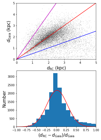
In the first step of our method, we selected RC candidates that lie in the two borderlines. The selected candidates may contain some contaminants, such as the red giants or dwarfs. We cross-match the selected RC candidates of all the catalogued clouds with the Gaia DR2 data (Gaia Collaboration et al., 2018). Two distances are simultaneously estimated for the individual RC candidates. One is Gaia distance obtained from the Gaia DR2 parallaxes (Lindegren et al., 2018), which can be treated as their ‘true’ distances. The other is RC distance estimated by Eqs. (1) and (2). If a selected candidate is not a RC, its RC distance will be over-estimated (for dwarfs) or underestimated (for giants) comparing to its Gaia distance . In the current work, we adopt the Gaia distances of stars from Bailer-Jones et al. (2018) and exclude all sources with Gaia DR2 distance uncertainties larger than 20 per cent. The comparison of these two distances is shown in Fig. 6. For most of the selected candidates, their RC distances are in good agreement with the Gaia ones. The mean and scatter of the differences are only 1.8 and 25.8 per cent, respectively. The contamination of the giants or dwarfs does not affect the determination of the RC tracks, and it does not affect the distance uncertainties.
Our distance estimates are ultimately based on the distance estimates of RCs. The dispersions of the intrinsic colour and absolute magnitude of the disk RCs are both 0.05 mag (Salaris & Girardi, 2002; Chen et al., 2017b; Plevne et al., 2020). Typically, for a point in the RC track located at = 2.5 mag and =13 mag, the corresponding distance uncertainty is about 7 per cent.
The extinction coefficient adopted in the current work is from Wang & Chen (2019), who obtained high-precision optical to mid-IR extinction coefficients based on RCs selected from the APOGEE survey. The uncertainty of the near-IR extinction coefficient is about 5 per cent (see also Alonso-García et al. 2017). For = 2 mag, the corresponding distance uncertainty is 2 per cent. Hence, to address the uncertainty of our resultant cloud distance, we adopt a systematic uncertainty of 7 per cent.

5.2 Spiral structure in the fourth Galactic quadrant
The spiral structure of the Milky Way is not yet well determined, especially for the fourth quadrant of the Galactic disk, due to the lack of spiral tracers with accurately determined distances (e.g., Xu et al. 2018; Reid et al. 2019). Giant molecular cloud has proven to be one of the best tracers of Galaxy spiral arms (e.g., Grabelsky et al. 1988; Xu et al. 2018). In our catalogue, the clouds are all giant molecular clouds having masses larger than 104 M⊙ (see Table 1). With their robust determined distances in this work, the spiral structure in the fourth Galactic quadrant may be better delineated.
In Fig. 7, we plot the projected distribution of the 169 giant molecular clouds in the Galactic plane. These clouds are located primarily in the Scutum-Centaurus Arm, the Normal Arm and the Near 3 kpc Arm. Some of the clouds seem to reside in the inter arm regions, which may be related with arm branches or spurs. To make a comparison, we over-plot those high-mass star-forming regions (HMSFRs) with trigonometric parallax measurements as listed in Reid et al. (2019) and those nearby molecule clouds with extinction distances as listed in Chen et al. (2020). Also shown in Fig. 7 are the best fitted spiral arm models from Reid et al. (2019) and Chen et al. (2019a), which are updated views of the Galaxy spiral structure.
It is shown that the Scutum-Centaurus Arm traced by our catalogued clouds deviates clearly from the best fitted model of Reid et al. (2019). The extensions of the Reid et al. spiral arms in the fourth Galactic quadrant seem to be less reliable, as they were determined by matching the observed spiral arm tangences rather than parallax measurements. As shown in the Fig. 1 of Reid et al. (2019), the HMSFRs with parallax distances are still very rare in the fourth Galactic quadrant.
Recently, Chen et al. (2019a) estimated the parameters of the Scutum-Centaurus Arm based on their large sample of O and early B-type stars with the Gaia results of parallaxes, and also the HMSFR sample of Xu et al. (2018) with trigonometric parallax measurements. From Fig. 7, it is clear that comparing to the model of the Scutum-Centaurus Arm from Reid et al. (2019), the Chen et al. model matches better to the distribution of our catalogued clouds. This is reasonable, since there are more spiral tracers having accurate distances in the fourth Galactic quadrant than that of Reid et al. (2019).
Similar situation is found for the Norma Arm, there are also a large deviation between the best fitted model of Reid et al. (2019) and our giant molecular cloud distribution. Finally, eight of our catalogued clouds are located near the 3 kpc Arm of Reid et al. (2019), which may confirm the robustness of their model of the Near 3 kpc Arm. To obtain more accurate spiral structure in the fourth Galactic quadrant, parallax measurements of more HMSFR masers are necessary. It would be also helpful to combine together the data of HMSFR masers, giant molecular clouds, O and early B-type stars in the analysis.
6 Conclusion
In this paper, we have estimated extinction distances to 169 giant molecular clouds in the fourth Galactic quadrant. Based on the near-IR photometry of 2MASS and VVV, we have selected 230 giant molecular clouds from Rice et al. (2016). For each cloud, we select the RC candidates from the CMD of the cloud overlapping sightline. Based on the RC candidates, we find the RC track to determine the extinction profile of the sightline. Using a simple extinction model, we have derived accurate distance of the cloud by fitting the extinction and distance relation along the sightline. As a result, we have obtained extinction distances to 169 clouds, which locate at distances between 2 and 11 kpc. The typical statistical error and the systematic uncertainty of the distances are 5 and 7 pre cent, respectively.
The result is a unique catalogue of distant molecular clouds in the inner Galaxy with robust directly-measured distances. Based on this catalogue, we have tested different spiral arm models from the literature. We find large deviations between the spatial distribution of our giant molecular clouds and the Scutum-Centaurus and the Norma arm models from Reid et al. (2019) in the Galactic fourth quadrant. To obtain more accurate spiral structure in the region, parallax measurements of more HMSFR masers are necessary.
Acknowledgements
This paper is published to commemorate the 60th anniversary of the Department of Astronomy, Beijing Normal University. We thank the anonymous referee for her/his useful comments. This work is partially supported by National Natural Science Foundation of China 11803029, U1531244, 11533002, 11833006, 11988101, 11933011, 11833009 and U1731308 and Yunnan University grant No. C176220100007. L.G.H thanks the support from the Youth Innovation Promotion Association CAS.
This publication makes use of data products from the Two Micron All Sky Survey, which is a joint project of the University of Massachusetts and the Infrared Processing and Analysis Center/California Institute of Technology, funded by the National Aeronautics and Space Administration and the National Science Foundation.
This work is based on data products from VVV Survey observations made with the VISTA telescope at the ESO Paranal Observatory under programme ID 179.B-2002.
Data availability
The data underlying this article are available in the article and in its online supplementary material.
References
- Alonso-García et al. (2017) Alonso-García, J., et al. 2017, ApJ, 849, L13
- Alves (2000) Alves, D. R. 2000, ApJ, 539, 732
- Bailer-Jones et al. (2018) Bailer-Jones, C. A. L., Rybizki, J., Fouesneau, M., Mantelet, G., & Andrae, R. 2018, AJ, 156, 58
- Chen et al. (1998) Chen, B., Vergely, J. L., Valette, B., & Carraro, G. 1998, A&A, 336, 137
- Chen et al. (2019a) Chen, B. Q., et al. 2019a, MNRAS, 487, 1400
- Chen et al. (2019b) Chen, B.-Q., et al. 2019b, MNRAS, 483, 4277
- Chen et al. (2020) Chen, B. Q., et al. 2020, MNRAS, 493, 351
- Chen et al. (2017a) Chen, B. Q., et al. 2017a, MNRAS, 472, 3924
- Chen et al. (2014) Chen, B. Q., et al. 2014, MNRAS, 443, 1192
- Chen et al. (2017b) Chen, Y. Q., Casagrande, L., Zhao, G., Bovy, J., Silva Aguirre, V., Zhao, J. K., & Jia, Y. P. 2017b, ApJ, 840, 77
- Dame et al. (2001) Dame, T. M., Hartmann, D., & Thaddeus, P. 2001, ApJ, 547, 792
- Foreman-Mackey et al. (2013) Foreman-Mackey, D., Hogg, D. W., Lang, D., & Goodman, J. 2013, PASP, 125, 306
- Gaia Collaboration et al. (2018) Gaia Collaboration, et al. 2018, A&A, 616, A1
- Gao et al. (2009) Gao, J., Jiang, B. W., & Li, A. 2009, ApJ, 707, 89
- Gonzalez et al. (2012) Gonzalez, O. A., Rejkuba, M., Zoccali, M., Valenti, E., Minniti, D., Schultheis, M., Tobar, R., & Chen, B. 2012, A&A, 543, A13
- Grabelsky et al. (1988) Grabelsky, D. A., Cohen, R. S., Bronfman, L., & Thaddeus, P. 1988, ApJ, 331, 181
- Green et al. (2015) Green, G. M., et al. 2015, ApJ, 810, 25
- Gregorio-Hetem (2008) Gregorio-Hetem, J. 2008, The Canis Major Star Forming Region, ed. B. Reipurth, Vol. 5, 1
- Grocholski & Sarajedini (2002) Grocholski, A. J. & Sarajedini, A. 2002, AJ, 123, 1603
- Güver et al. (2010) Güver, T., Özel, F., Cabrera-Lavers, A., & Wroblewski, P. 2010, ApJ, 712, 964
- Lindegren et al. (2018) Lindegren, L., et al. 2018, A&A, 616, A2
- Marshall et al. (2009) Marshall, D. J., Joncas, G., & Jones, A. P. 2009, ApJ, 706, 727
- Marshall et al. (2006) Marshall, D. J., Robin, A. C., Reylé, C., Schultheis, M., & Picaud, S. 2006, A&A, 453, 635
- Minniti et al. (2010) Minniti, D., et al. 2010, New A., 15, 433
- Miville-Deschênes et al. (2017) Miville-Deschênes, M.-A., Murray, N., & Lee, E. J. 2017, ApJ, 834, 57
- Plevne et al. (2020) Plevne, O., Önal Ta\textcommabelows, Ö., Bilir, S., & Seabroke, G. M. 2020, ApJ, 893, 108
- Reid et al. (2019) Reid, M. J., et al. 2019, The Astrophysical Journal, 885, 131
- Rice et al. (2016) Rice, T. S., Goodman, A. A., Bergin, E. A., Beaumont, C., & Dame, T. M. 2016, The Astrophysical Journal, 822, 52
- Roman-Duval et al. (2009) Roman-Duval, J., Jackson, J. M., Heyer, M., Johnson, A., Rathborne, J., Shah, R., & Simon, R. 2009, ApJ, 699, 1153
- Saito et al. (2012) Saito, R. K., et al. 2012, A&A, 537, A107
- Salaris & Girardi (2002) Salaris, M. & Girardi, L. 2002, MNRAS, 337, 332
- Schlafly et al. (2014) Schlafly, E. F., et al. 2014, ApJ, 786, 29
- Shan et al. (2019) Shan, S.-S., Zhu, H., Tian, W.-W., Zhang, H.-Y., Yang, A.-Y., & Zhang, M.-F. 2019, Research in Astronomy and Astrophysics, 19, 092
- Shan et al. (2018) Shan, S. S., Zhu, H., Tian, W. W., Zhang, M. F., Zhang, H. Y., Wu, D., & Yang, A. Y. 2018, ApJS, 238, 35
- Skrutskie et al. (2006) Skrutskie, M. F., et al. 2006, AJ, 131, 1163
- Soto et al. (2013) Soto, M., et al. 2013, A&A, 552, A101
- Wang & Chen (2019) Wang, S. & Chen, X. 2019, ApJ, 877, 116
- Wang et al. (2020) Wang, S., Zhang, C., Jiang, B., Zhao, H., Chen, B., Chen, X., Gao, J., & Liu, J. 2020, arXiv e-prints, arXiv:2005.08270
- Xu et al. (2018) Xu, Y., Hou, L.-G., & Wu, Y.-W. 2018, Research in Astronomy and Astrophysics, 18, 146
- Yan et al. (2019) Yan, Q.-Z., Yang, J., Sun, Y., Su, Y., & Xu, Y. 2019, ApJ, 885, 19
- Yu et al. (2019) Yu, B., Chen, B. Q., Jiang, B. W., & Zijlstra, A. 2019, MNRAS, 488, 3129
- Zhao et al. (2018) Zhao, H., Jiang, B., Gao, S., Li, J., & Sun, M. 2018, ApJ, 855, 12
- Zhao et al. (2020) Zhao, H., Jiang, B., Li, J., Chen, B., Yu, B., & Wang, Y. 2020, ApJ, 891, 137
- Zucker et al. (2019) Zucker, C., Speagle, J. S., Schlafly, E. F., Green, G. M., Finkbeiner, D. P., Goodman, A. A., & Alves, J. 2019, ApJ, 879, 125