The detection of a hot molecular core in the extreme outer Galaxy
Abstract
Interstellar chemistry in low metallicity environments is crucial to understand chemical processes in the past metal-poor universe. Here we report the first detection of a hot molecular core in the extreme outer Galaxy, which is an excellent laboratory to study star formation and interstellar medium in a Galactic low-metallicity environment. The target star-forming region, WB89-789, is located at the galactocentric distance of 19 kpc. Our ALMA observations have detected a variety of carbon-, oxygen-, nitrogen-, sulfur-, and silicon-bearing species, including complex organic molecules (COMs) containing up to nine atoms, towards a warm (100 K) and compact ( 0.03 pc) region associated with a protostar (8 103 L☉). A comparison of fractional abundances of COMs relative to CH3OH between the outer Galactic hot core and an inner Galactic counterpart shows a remarkable similarity. On the other hand, the molecular abundances in the present source do not resemble those of low-metallicity hot cores in the Large Magellanic Cloud. The detection of another embedded protostar associated with high-velocity SiO outflows is also reported.
1 Introduction
Understanding the star formation and interstellar medium (ISM) at low metallicity is crucial to unveil physical and chemical processes in the past Galactic environment or those in high-redshift galaxies, where the metallicity was significantly lower compared to the present-day solar neighborhood.
Hot cores are one of the early stages of star formation and they play a key role in the formation of chemical complexity of the ISM. Physically, hot cores are defined as having small source size (0.1 pc), high density (106 cm-3), and warm gas/dust temperature (100 K) (e.g., van Dishoeck & Blake, 1998; Kurtz et al., 2000). Chemistry of hot cores is characterized by sublimation of ice mantles, which accumulated in the course of star formation. In cold molecular clouds and prestellar cores, gaseous molecules and atoms are frozen onto dust grains. With increasing dust temperatures by star formation activities, chemical reaction among heavy species become active on grain surfaces to form larger complex molecules (e.g., Garrod & Herbst, 2006). In addition, sublimated molecules, such as CH3OH and NH3, are subject to further gas-phase reactions (e.g., Nomura & Millar, 2004; Taquet et al., 2016). As a result, warm and dense gas around protostars become chemically rich, and embedded protostars are observed as one of the most powerful molecular line emitters, which is called a hot core. They are important targets for astrochemical studies of star-forming regions, because a variety of molecular species, including complex organic molecules (COMs), are often detected in hot cores (Herbst & van Dishoeck, 2009, and references therein). Thus detailed studies on chemical properties of hot cores are important for understanding complex chemical processes triggered by star formation.
Recent ALMA (Atacama Large Millimeter/submillimeter Array) observations of hot molecular cores in a nearby low metallicity galaxy, the Large Magellanic Cloud (LMC), have suggested that the metallicity has a significant effect on their molecular compositions (Shimonishi et al., 2016b, 2020; Sewiło et al., 2018); cf., the metallicity of the LMC is 1/2-1/3 of the solar neighborhood. A comparison of molecular abundances between LMC and Galactic hot cores suggests that organic molecules (e.g., CH3OH, a classical hot core tracer) show a large abundance variation in low-metallicity hot cores (Shimonishi et al., 2020). There are organic-poor hot cores that are unique in the LMC (Shimonishi et al., 2016b), while there are relatively organic-rich hot cores, where the abundances of organic molecules roughly scale with the metallicity (Sewiło et al., 2018). Astrochemical simulations for low-metallicity hot cores suggest that dust temperature during the initial ice-forming stage would play a key role for making the chemical diversity of organic molecules (Acharyya & Herbst, 2018; Shimonishi et al., 2020). On the other hand, sulfur-bearing molecules such as SO2 and SO are commonly detected in known LMC hot cores and their molecular abundances roughly scale with the metallicity of the LMC. Although the reason is still under debate, the results suggest that SO2 can be an alternative molecular species to trace hot core chemistry in metal-poor environments.
The above results suggest that molecular abundances in hot cores do not always simply scale with the elemental abundances of their parent environments. However, it is still unclear if the observed chemical characteristics of LMC hot cores are common in other low metallicity environments or they are uniquely seen only in the LMC. Currently, known low-metallicity hot core samples are limited to those in the LMC. It is thus vital to understand universal characteristics of interstellar chemistry by studying chemical compositions of star-forming cores in diverse metallicity environments.
Recent surveys (e.g., Anderson et al., 2015, 2018; Izumi et al., 2017; Wenger et al., 2021) have found a number of (10-20) star-forming region candidates in the extreme outer Galaxy, which is defined as having galactocentric distance () larger than 18 kpc (Yasui et al., 2006; Kobayashi et al., 2008). The extreme outer Galaxy has a very different environment from those in the solar neighborhood, with lower metallicity (less than -0.5 dex, Fernández-Martín et al., 2017; Wenger et al., 2019), lower gas density (e.g., Nakanishi & Sofue, 2016), and small or no perturbation from spiral arms. Such an environment is of great interest for studies of the star formation and ISM in the early phase of the Milky Way formation and those in dwarf galaxies (Ferguson et al., 1998; Kobayashi et al., 2008). The low metallicity environment is in common with the Magellanic Clouds, and thus the extreme outer Galaxy is an ideal laboratory to test the universality of the low metallicity molecular chemistry observed in the LMC and SMC.
Among star-forming regions in the extreme outer Galaxy, WB89-789 (IRAS 06145+1455; 06h17m242, 145442, J2000) has particularly young and active nature (Brand & Wouterloot, 1994). It is located at the galactocentric distance of 19.0 kpc and the distance from Earth is 10.7 kpc (based on optical spectroscopy of a K3 III star, Brand & Wouterloot, 2007). The metallicity of WB89-789 is estimated to be a factor of four lower than the solar value according to the Galactic oxygen abundance gradient reported in the literature (Fernández-Martín et al., 2017; Wenger et al., 2019; Bragança et al., 2019; Arellano-Córdova et al., 2020, 2021). The region is associated with dense clouds traced by CS and CO (Brand & Wouterloot, 2007). The total mass of the cloud is estimated to be 6 103 M☉ for a 10 pc diameter area (Brand & Wouterloot, 1994). An H2O maser is detected towards the region (Wouterloot et al., 1993), but no centimeter radio continuum is found (Brand & Wouterloot, 2007). Several class I protostar candidates are identified by previous infrared observations (Brand & Wouterloot, 2007).
We here report the first detection of a hot molecular core in the extreme outer Galaxy based on submillimeter observations towards WB89-789 with ALMA. Section 2 describes the details of the target source, observations, and data reduction. The observed molecular line spectra and images, as well as analyses of physical and chemical properties of the source, are presented in Section 3. Discussion about the properties of the hot core and comparisons of molecular abundances with known Galactic and LMC hot cores are given in Section 4. This section also presents the detection of another embedded protostar with high-velocity outflows in the WB89-789 region. The conclusions are given in Section 5.
| Observation | On-source | Mean | Number | Baseline | Channel | ||||
|---|---|---|---|---|---|---|---|---|---|
| Date | Time | PWVaaPrecipitable water vapor. | of | Min | Max | Bem sizebbThe average beam size of continuum achieved by TCLEAN with the Briggs weighting and the robustness parameter of 0.5. Note that we use a common circular restoring beam size of 050 for Band 6 and 7 data to construct the final images. | MRSccMaximum Recoverable Scale. | Spacing | |
| (min) | (mm) | Antennas | (m) | (m) | ( ) | () | |||
| Band 6 | 2018 Dec 6 – | 115.5 | 0.5–1.5 | 45–49 | 15.1 | 783.5 | 0.41 0.50 | 5.6 | 0.98 MHz |
| (250 GHz) | 2019 Apr 16 | (1.2 km s-1) | |||||||
| Band 7 | 2018 Apr 30 – | 64.1 | 0.6–1.0 | 43-44 | 15.1 | 500.2 | 0.46 0.52 | 5.4 | 0.98 MHz |
| (350 GHz) | 2018 Aug 22 | (0.85 km s-1) | |||||||
2 Target, observations, and data reduction
2.1 Target
The target star-forming region is WB89-789 (Brand & Wouterloot, 1994). The region contains three Class I protostar candidates identified by near-infrared observations (Brand & Wouterloot, 2007), and one of them is a main target of the present ALMA observations. The region observed with ALMA is indicated on a near-infrared two-color image shown in Figure 1. The observed position is notably reddened compared with other parts of WB89-789.

2.2 Observations
Observations were conducted with ALMA in 2018 and 2019 as a part of the Cycle 5 (2017.1.01002.S) and Cycle 6 (2018.1.00627.S) programs (PI: T. Shimonishi). A summary of the present observations is shown in Table 1. The pointing center of antennas is RA = 06h17m23s and Dec = 145441 (ICRS). The total on-source integration time is 115.5 minutes for Band 6 data and 64.1 minutes for Band 7. Flux and bandpass calibrators are J0510+1800, J0854+2006, and J0725-0054 for Band 6, while J0854+2006 and J0510+1800 for Band 7, respectively. Phase calibrators are J0631+2020 and J0613+1708 for Band 6 and J0643+0857 and J0359+1433 for Band 7. Four spectral windows are used to cover the sky frequencies of 241.40–243.31, 243.76-245.66, 256.90–258.81, and 258.76–260.66 GHz for Band 6, while 337.22–339.15, 339.03-340.96, 349.12–351.05, and 350.92–352.85 GHz for Band 7. The channel spacing is 0.98 MHz, which corresponds to 1.2 km s-1 for Band 6 and 0.85 km s-1 for Band 7. The total number of antennas is 45–49 for Band 6 and 43–44 for Band 7. The minimum–maximum baseline lengths are 15.1–783.5 m for Band 6 and 15.1–500.2 m for Band 7. A full-width at half-maximum (FWHM) of the primary beam is about 25 for Band 6 and 18 for Band 7.
2.3 Data reduction
Raw data is processed with the Common Astronomy Software Applications (CASA) package. We use CASA 5.4.0 (Band 6) and 5.1.1 (Band 7) for the calibration and CASA 5.5.0 for the imaging. The synthesized beam sizes of 039–042 049–052 with a position angle of -36 degree for Band 6 and 045–046 051–052 with a position angle of - 54 degree for Band 7 are achieved with the Briggs weighting and the robustness parameter of 0.5. In this paper, we use a common circular restoring beam size of 050, which corresponds to 0.026 pc (5350 au) at the distance of WB89-789. The synthesized images are corrected for the primary beam pattern using the impbcor task in CASA. The continuum image is constructed by selecting line-free channels. Before the spectral extraction, the continuum emission is subtracted from the spectral data using the CASA’s uvcontsub task.
The spectra and continuum flux are extracted from the 050 diameter circular region centered at RA = 06h17m24073 and Dec = 14544227 (ICRS), which corresponds to the submillimeter continuum center of the target and is equivalent to the hot core position. Hereafter, the source is referred to as WB89-789 SMM1.
| 2 atoms | 3 atoms | 4 atoms | 5 atoms | 6 atoms | 7 atoms | 8 atoms | 9 atoms |
|---|---|---|---|---|---|---|---|
| CN | HDO | H2CO | c-C3H2 | CH3OH | CH3CHO | HCOOCH3 | CH3OCH3 |
| NO | H13CO+ | HDCO | HC3N | 13CH3OH | c-C2H4O | C2H5OH | |
| CS | HC18O+ | D2CO | H2CCO | CH2DOH | C2H5CN | ||
| C34S | H13CN | HNCO | HCOOH | CH3CN | |||
| C33S | HC15N | H2CS | NH2CO | ||||
| SO | CCH | ||||||
| 34SO | SO2 | ||||||
| 33SO | 34SO2 | ||||||
| SiO | OCS | ||||||
| 13OCS |
3 Results and analysis
3.1 Spectra
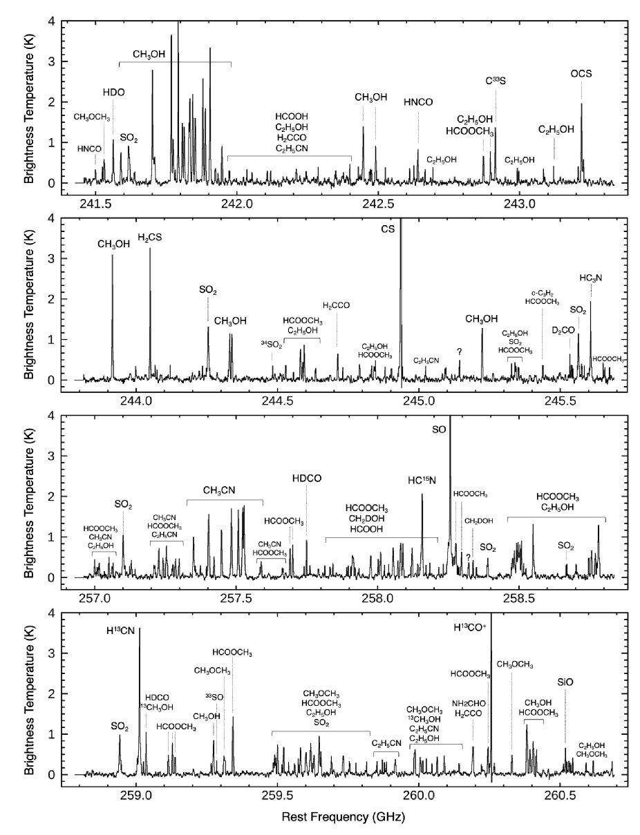
Figures 2–3 show submillimeter spectra extracted from the continuum center of WB89-789 SMM1. Spectral lines are identified with the aid of the Cologne Database for Molecular Spectroscopy111https://www.astro.uni-koeln.de/cdms (CDMS, Müller et al., 2001, 2005) and the molecular database of the Jet Propulsion Laboratory222http://spec.jpl.nasa.gov (JPL, Pickett et al., 1998).
Line parameters are measured by fitting a Gaussian profile to detected lines. We estimate the peak brightness temperature, the FWHM, the LSR velocity, and the integrated intensity for each line based on the fitting. For spectral lines for which a Gaussian profile does not fit well, their integrated intensities are calculated by directly integrating the spectrum over the frequency region of emission. Full details of the line fitting can be found in Appendix A (Tables of measured line parameters) and Appendix B (Figures of fitted spectra). The table also contains the estimated upper limits on important non-detection lines.
A variety of carbon-, oxygen-, nitrogen-, sulfur-, and silicon-bearing species, including COMs containing up to nine atoms, are detected from WB89-789 SMM1 (see Table 2). Multiple high excitation lines (upper state energy 100 K) are detected for many species. Measured line widths are typically 3–6 km s-1. Most of lines consist of a single velocity component, but SiO has doppler shifted components at 5 km s-1 as indicated in Figure 14 in Appendix B.

3.2 Images
Figures 4–5 show synthesized images of continuum and molecular emission lines observed toward the target region. The images are constructed by integrating spectral data in the velocity range where the emission is detected. Most molecular lines, except for those of molecular radicals CN, CCH, and NO, have their intensity peak at the continuum center, which corresponds to the position of a hot core. Simple molecules such as H13CO+, H13CN, CS, and SO are extended compared to the beam size. Secondary intensity peaks are also seen in those species. Complex molecules and HDO are concentrated at the hot core position. A characteristic symmetric distribution is seen in SiO. Further discussion about the distribution of the observed emission is presented in Section 4.2.


3.3 Derivation of column densities, gas temperatures, and molecular abundances
3.3.1 Rotation diagram analysis
Column densities and rotation temperatures are estimated based on the rotation diagram analysis for the molecular species where multiple transitions with different excitation energies are detected (Figure 6). We here assume an optically thin condition and the local thermodynamic equilibrium (LTE). We use the following formulae based on the standard treatment of the rotation diagram analysis (e.g., Sutton et al., 1995; Goldsmith & Langer, 1999):
| (1) |
where
| (2) |
and is a column density of molecules in the upper energy level, is the degeneracy of the upper level, is the Boltzmann constant, is the integrated intensity estimated from the observations, is the transition frequency, is the line strength, is the dipole moment, is the rotational temperature, is the upper state energy, is the total column density, and is the partition function at . All the spectroscopic parameters required in the analysis are extracted from the CDMS or JPL database. Derived column densities and rotation temperatures are summarized in Table 3.
Most molecular species are well fitted by a single temperature component. Data points in diagrams of CH3CN and C2H5CN are relatively scattered. For CH3OH, CH3CN, HNCO, SO2, and HCOOCH3, transitions with relatively large values at low (300 K) are excluded from the fit in order to avoid possible effect of optical thickness (see gray points in Fig. 6).
Complex organic molecules, HDO, and SO2 show high rotation temperatures (130 K). This suggests that they are originated from a warm region associated with a protostar. On the other hand, C33S and D2CO, and H2CS show lower temperatures, suggesting that they arise from a colder region in the outer part of the protostellar envelope.

3.3.2 Column densities of other molecules
Column densities of molecular species for which rotation diagram analysis is not applicable are estimated from Equation 1 after solving it for . Their rotation temperatures are estimated as follows, by taking into account that the sight-line of WB89-789 SMM1 contains both cold and warm gas components as described in Section 3.3.1.
The rotation temperature of C33S is applied to those of CS and C34S, considering a similar distribution of isotopologues. Similarly, the rotation temperature of D2CO is applied to H2CO and HDCO, and that of SO2 to 34SO2. For other species, we assume that molecules with an extended spatial distribution trace a relatively low-temperature region rather than a high-temperature gas associated with a hot core. CN, CCH, H13CO+, HC18O+, H13CN, HC15N, NO, SiO, 34SO, 33SO, and c-C3H2 correspond to this case. We assume a rotation temperature of 35 K for those species, which is roughly equivalent to that of C33S.
High gas temperatures are observed for COMs, SO2, and HDO, which are associated with a compact hot core region. Average temperature of those species is 200 K. We assume this temperature for column density estimates (including upper limit) of c-C2H4O, HC3N, 13CH3CN, 13OCS, and CH3SH. Estimated column densities are summarized in Table 3.
We have also estimated column densities of selected species based on non-LTE calculations with RADEX (van der Tak et al., 2007). For input parameters, we use the H2 gas density of 2.1 107 cm-3 according to our estimate in Section 3.3.3 and the background temperature of 2.73 K. Kinetic temperatures are assumed to be the same as temperatures tabulated in Table 3. The line intensities and widths are taken from the tables in Appendix A 333The following lines are used for non-LTE calculation with RADEX; H13CO+(3–2), HC18O+(4–3), H2CO(51,5–41,4), c-C3H2(32,1–21,2), CN(N = 3–2, J = –, F = –), H13CN(3–2), HC15N(3–2), HC3N(27–26), NO(J = –, = , F = +–-), CH3CN(140–130), SiO(6–5), CS(5–4), OCS(20–19), H2CS(71,6–61,5), SO( = 66–55), and CH3OH(75 E–65 E). . We assume an empirical 10 uncertainty for input line intensities. The resultant column densities are summarized in Table 3. The calculated non-LTE column densities are reasonably consistent with the LTE estimates.
3.3.3 Column density of H2, dust extinction, and gas mass
A column density of molecular hydrogen () is estimated from the dust continuum data. We use the following equation to calculate based on the standard treatment of optically thin dust emission:
| (3) |
where is the continuum flux density per beam solid angle as estimated from the observations, is the mass absorption coefficient of dust grains coated by thin ice mantles at 1200/870 m as taken from Ossenkopf & Henning (1994) and we here use 1.07 cm2 g-1 for 1200 m and 1.90 cm2 g-1 for 870 m, is the dust temperature and is the Planck function, is the dust-to-gas mass ratio, is the mean atomic mass per hydrogen (1.41, according to Cox, 2000), and is the hydrogen mass. We use the dust-to-gas mass ratio of 0.002, which is obtained by scaling the Galactic value of 0.008 by the metallicity of the WB89-789 region.
A line of sight towards a hot core contain dust grains with different temperatures because of the temperature gradient in a protostellar envelope. Representative dust temperature (i.e. mass-weighted average temperature) would fall somewhere in between that of a warm inner region and a cold outer region. Shimonishi et al. (2020) presented a detailed analysis of effective dust temperature in the sight-line of a low-metallicity hot core in the LMC, based on a comparison of derived by submillimeter dust continuum with the above method, model fitting of spectral energy distributions (SEDs), and the 9.7 m silicate dust absorption depth. The paper concluded that = 60 K for the dust continuum analysis yields the value which is consistent with those obtained by other different methods. This temperature corresponds to an intermediate value between a cold gas component (50 K) represented by SO and a warm component (150 K) represented by CH3OH and SO2 in this LMC hot core. The present hot core, WB89-789 SMM1, harbors similar temperature components as discussed in Sections 3.3.1 and 3.3.2. We thus applied = 60 K for the present source. The continuum brightness of SMM1 is measured to be 11.33 0.05 mJy/beam for 1200 m and 28.0 0.2 mJy/beam for 870 m (3 uncertainty). Based on the above assumption, we obtain = 1.6 1024 cm-2 for 1200 m and = 1.2 1024 cm-2 for the 870 m. The value changes by a factor of up to 1.6 when the assumed is varied between 40 K and 90 K.
Alternatively, a column density of molecular hydrogen can be determined by the model fitting of the observed spectral energy distribution (SED). The best-fit SED discussed in Section 4.1 yields = 184 mag. We here use a standard value of / = 5.8 1021 cm-2 mag-1 (Draine, 2003) and a slightly high / ratio of 4 for dense clouds (Whittet et al., 2001). Taking into account a factor of four lower metallicity, we obtain / = 2.9 1021 cm-2 mag-1, where we assume that all the hydrogen atoms are in the form of H2. Using this conversion factor, we obtain = 5.3 1023 cm-2. This is similar to the derived from the aforementioned method assuming = 150 K. Such may be somewhat high as a typical dust temperature in the line of sight, but it is not very unrealistic value given the observed temperature range of molecular gas towards WB89-789 SMM1.
In this paper, we use = 1.1 1024 cm-2 as a representative value, which corresponds to the average of derived by the dust continuum data and the SED fitting. This corresponds to = 380 mag using the above conversion factor. Assuming the source diameter of 0.026 pc and the uniform spherical distribution of gas around a protostar, we estimate the gas number density to be = 2.1 107 cm-3, where the total gas mass of 13 M☉ is enclosed.
3.3.4 Fractional abundances and isotope abundance ratios
Fractional abundances with respect to H2 are shown in Table 4, which are calculated based on column densities estimated in Sections 3.3.1–3.3.3. The fractional abundances normalized by the CH3OH column density are also discussed in Sections 4.3-4.4, because of the non-negligible uncertainty associated with (see Section 3.3.3).
Abundances of HCO+, HCN, SO, CS, OCS, and CH3OH are estimated from their isotopologues, H13CO+, H13CN, 34SO, C34S, O13CS, and 13CH3OH. Detections of isotopologue species for SO, CS, OCS, and CH3OH imply that the main species would be optically thick. Isotope abundance ratios of 12C/13C = 150 and 32S/33S = 35 are assumed, which are obtained by extrapolating the relationship between isotope ratios and galactocentric distances reported in Wilson & Rood (1994) and Humire et al. (2020) to = 19 kpc.
Abundance ratios are derived for several rare isotopologues; we obtain CH2DOH/CH3OH = 0.011 0.002, D2CO/HDCO = 0.45 0.10, 34SO/33SO = 5 1, C34S/C33S = 2 1, and 32SO2/34SO2 = 20 4. The 32SO2/34SO2 ratio in WB89-789 SMM1 is similar to the solar 32S/34S ratio (22, Wilson & Rood, 1994), although we expect a slightly higher value in the outer Galaxy due to the 32S/34S gradient in the Galaxy (Chin et al., 1996; Humire et al., 2020). Astrophysical implication for the deuterated species are discussed in Section 4.4.
The rotation diagram of CH3CN is rather scattered. Although its isotopologue line is not detected, optical thickness might affect the column density estimate, as CH3CN is often optically thick in hot cores (e.g., Fuente et al., 2014). To obtain a possible range of its column density, we use the rotation diagram of 12CH3CN data to estimate a lower limit and the non-detection of the 13CH3CN(190–180) line at 339.36630 GHz ( = 163 K) for an upper limit.
We have also repeated the analysis for the spectra extracted from a 0.1 pc (193) diameter region at the hot core position, for the sake of comparison with LMC hot cores (see Section 4.4). Those abundances are also summarized in Table 4. The abundances for a 0.1 pc area do not drastically vary from those for a 0.026 pc area. Molecules with compact spatial distribution (e.g., COMs) tend to decrease their abundances by a factor of 2–3 in the 0.1 pc data due to the beam dilution effect. In contrast, those with extended spatial distributions and intensity peaks outside the hot core region (H13CO+, CCH, CN, and NO) increases by a factor of 2 in the 0.1 pc data.
| Molecule | rot | (X) | (X) non-LTE | Size |
|---|---|---|---|---|
| (K) | (cm-2) | (cm-2) | () | |
| H2 | 1.1 1024 | 0.85ccSize of continuum emission. | ||
| H13CO+ | 35 | (7.0 0.1) 1012 | (7.6 0.9) 1012 | 1.5ddAssociated with extended component. |
| HC18O+ | 35 | (5.8 0.9) 1011 | (5.7 0.6) 1011 | 1.18ddAssociated with extended component. |
| CCH | 35 | (2.7 0.1) 1014 | 2ddAssociated with extended component. | |
| c-C3H2 | 35 | (9.5 2.2) 1013 | (8.2 0.9) 1013aaAssuming ortho/para ratio of three. | 1ddAssociated with extended component. |
| H2CO | 39 | (1.1 0.1) 1014 | (1.3 0.1) 1014aaAssuming ortho/para ratio of three. | 1.5ddAssociated with extended component. |
| HDCO | 39 | (5.1 0.3) 1013 | 1ddAssociated with extended component. | |
| D2CO | 39 | (2.3 0.5) 1013 | 1ddAssociated with extended component. | |
| CN | 35 | (3.3 0.2) 1014 | (2.5 0.3) 1014 | 2ddAssociated with extended component. |
| H13CN | 35 | (1.2 0.1) 1013 | (1.1 0.1) 1013 | 0.92ddAssociated with extended component. |
| HC15N | 35 | (6.3 0.2) 1012 | (5.8 0.6) 1012 | 0.75ddAssociated with extended component. |
| HC3N | 200 | (2.7 0.3) 1013 | (2.1 0.2) 1013 | 0.65 |
| NO | 35 | (9.0 2.5) 1014 | (8.9 0.9) 1014 | 1.5ddAssociated with extended component. |
| HNCO | 237 | (3.0 0.2) 1014 | 0.54 | |
| CH3CN | 279 | (1.8 0.1) 1014 | (8.6 0.8) 1013 | 0.51 |
| 13CH3CN | 200 | 5 1012 | ||
| C2H5CN | 130 | (6.3 1.7) 1013 | 0.52 | |
| NH2CO | 140 | (4.2 0.7) 1013 | 0.56 | |
| SiO | 35 | (2.5 0.2) 1012 | (2.5 0.3) 1012 | 0.65 |
| CS | 36 | (1.5 0.2) 1014 | (2.0 0.3) 1014 | 1.5 |
| C34S | 36 | (3.1 0.1) 1013 | 0.70 | |
| C33S | 36 | (1.5 0.2) 1013 | 0.61 | |
| OCS | 106 | (6.5 0.5) 1014 | (6.4 0.7) 1014 | 0.55 |
| 13OCS | 200 | (8.7 2.4) 1013 | 0.45 | |
| H2CS | 43 | (1.5 0.1) 1014 | (1.4 0.2) 1014aaAssuming ortho/para ratio of three. | 0.62 |
| SO | 35 | (4.0 0.3) 1014 | (4.5 0.5) 1014 | 0.70ddAssociated with extended component. |
| 34SO | 35 | (5.9 0.1) 1013 | 0.66 | |
| 33SO | 35 | (1.1 0.1) 1013 | 0.53 | |
| SO2 | 166 | (1.2 0.1) 1015 | 0.53 | |
| 34SO2 | 166 | (5.9 0.9) 1013 | 0.51 | |
| CH3SH | 200 | 3 1014 | ||
| HDO | 217 | (2.2 0.2) 1015 | 0.52 | |
| CH3OH | 245 | (1.9 0.1) 1016 | (2.6 0.1) 1016bbAssuming E-CH3OH/A-CH3OH ratio of unity (Wirström et al., 2011). | 0.51 |
| 13CH3OH | 181 | (2.8 0.2) 1015 | 0.46 | |
| CH2DOH | 155 | (4.6 0.3) 1015 | 0.52 | |
| HCOOCH3 | 181 | (8.6 0.4) 1015 | 0.51 | |
| CH3OCH3 | 137 | (2.6 0.1) 1015 | 0.52 | |
| C2H5OH | 136 | (9.6 1.3) 1014 | 0.50 | |
| CH3CHO | 192 | (6.4 0.8) 1014 | 0.49 | |
| trans-HCOOH | 71 | (2.7 0.6) 1014 | 0.58 | |
| cis-HCOOH | 69 | (2.4 1.2) 1013 | 0.49 | |
| H2CCO | 92 | (1.0 0.2) 1014 | 0.55 | |
| c-C2H4O | 200 | (8.9 2.0) 1013 | 0.47 |
| Molecule | (X)/ | |
|---|---|---|
| 0.026 pc area | 0.1 pc area | |
| HCO+aaEstimated from 13C isotopologue with 12C/13C = 150 | (9.5 3.2) 10-10 | (1.5 0.3) 10-9 |
| H2CO | (1.0 0.3) 10-10 | (1.2 0.1) 10-10 |
| HDCO | (4.7 1.3) 10-11 | (3.9 0.2) 10-11 |
| D2CO | (2.1 0.7) 10-11 | (2.0 0.3) 10-11 |
| C2H | (2.5 0.7) 10-10 | (5.8 1.2) 10-10 |
| c-C3H2 | (8.6 3.1) 10-11 | (5.9 1.2) 10-11 |
| CN | (3.0 0.8) 10-10 | (6.6 1.3) 10-10 |
| HCNaaEstimated from 13C isotopologue with 12C/13C = 150 | (1.7 0.6) 10-9 | (1.2 0.3) 10-9 |
| HC3N | (2.5 0.7) 10-11 | (1.4 0.1) 10-11 |
| NO | (8.1 3.2) 10-10 | (1.6 0.1) 10-9 |
| HNCO | (2.7 0.8) 10-10 | (7.1 0.6) 10-11 |
| CH3CNbbRotation diagram analysis of CH3CN is used to derive a lower limit and the non-detection of 13CH3CN for an upper limit. | (4.2 2.7) 10-10 | (3.7 2.8) 10-10 |
| C2H5CN | (5.8 2.2) 10-11 | (2.4 0.9) 10-11 |
| NH2CHO | (3.8 1.2) 10-11 | (1.8 0.1) 10-11 |
| SiO | (2.2 0.6) 10-12 | (1.2 0.1) 10-12 |
| CSccEstimated from 34S isotopologue with 32S/34S = 35 | (9.7 3.3) 10-10 | (6.4 1.3) 10-10 |
| SOccEstimated from 34S isotopologue with 32S/34S = 35 | (1.9 0.5) 10-9 | (1.3 0.3) 10-9 |
| OCSaaEstimated from 13C isotopologue with 12C/13C = 150 | (1.2 0.5) 10-8 | (4.1 1.4) 10-9 |
| H2CS | (1.4 0.4) 10-10 | (9.0 1.0) 10-11 |
| SO2 | (1.1 0.3) 10-9 | (2.9 0.1) 10-10 |
| CH3SH | 3 10-10 | 2 10-10 |
| HDO | (2.0 0.6) 10-9 | (7.7 0.9) 10-10 |
| CH3OHaaEstimated from 13C isotopologue with 12C/13C = 150 | (3.8 1.3) 10-7 | (1.7 0.3) 10-7 |
| CH2DOH | (4.2 1.2) 10-9 | (1.5 0.2) 10-9 |
| HCOOCH3 | (7.8 2.2) 10-9 | (3.0 0.2) 10-9 |
| CH3OCH3 | (2.3 0.6) 10-9 | (1.0 0.1) 10-9 |
| C2H5OH | (8.7 2.7) 10-10 | (3.3 0.8) 10-10 |
| CH3CHO | (5.8 1.8) 10-10 | (2.1 0.4) 10-10 |
| HCOOHddSum of and species. | (2.7 1.0) 10-10 | (1.2 0.4) 10-10 |
| H2CCO | (9.2 3.0) 10-11 | (3.7 0.9) 10-11 |
| c-C2H4O | (8.1 2.8) 10-11 | (5.9 1.2) 10-11 |
Note. — Uncertainties and upper limits are of the 2 level. Column densities of molecules for a 0.026 pc area are summarized in Table 3. An empirical uncertainty of 30 is assumed for .
4 Discussion
4.1 Hot molecular core and protostar associated with WB89-789 SMM1
The nature of WB89-789 SMM1 is characterized as (i) the compact distribution of warm gas (0.03 pc, see Section 4.2), (ii) the high gas temperature that can trigger the ice sublimation (100 K, Section 3.3.1), (iii) the high density (2 107 cm-3, Section 3.3.3), (iv) the association with a luminous protostar (see below), and (v) the presence of chemically rich molecular gas. Those properties suggest that the source is associated with a hot molecular core.
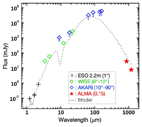
Figure 7 shows a SED of SMM1, where the data are collected from available databases and literatures (Brand & Wouterloot, 2007; Wright et al., 2010; Yamamura et al., 2010). The bolometric luminosity of the source is estimated to be 8.4 103 L☉ based on the SED fitting with the model of Robitaille et al. (2007). This luminosity is equivalent to a stellar mass of about 10 M☉ according to the mass-luminosity relationship of zero age main sequence (ZAMS) stars (Zinnecker & Yorke, 2007).
Note that far-infrared data, which is important for the luminosity determination of embedded sources, is insufficient for SMM1. Only upper limits are provided due to the low angular resolution of available AKARI FIS all-sky survey data. Thus the derived luminosity (and therefore mass) may be lower than the current estimate. Future high spatial resolution infrared observations in those missing wavelengths are highly required.
Alternatively, we can estimate the luminosity of SMM1 by scaling the luminosity of a low-metallicity LMC hot core, ST16, whose SED is well determined based on a comprehensive infrared dataset from 1 to 1200 m (Shimonishi et al., 2020). This LMC hot core has a total luminosity of 3.1 105 L☉ and a -band magnitude ([]) of 13.4 mag at 50 kpc, while SMM1 has [] = 14.7 mag at 10.7 kpc. Scaling the luminosity of ST16 with the distance and -band magnitude, we obtain 4.3 103 L☉ for SMM1, which is a factor of two lower than the estimate by the SED fitting. In either case, present estimates suggest that the luminosity of SMM1 would correspond to the lower-end of high-mass ZAMS or upper-end of intermediate-mass ZAMS.

4.2 Distribution of molecular line emission and dust continuum
The observed emission lines and continuum show different spatial distributions depending on species. Those distributions have important clues to understand their origins. A schematic illustration of the temperature structure and molecular gas distribution in WB89-789 SMM1 are shown in Figure 8 based on the discussion in this section.
We have estimated the spatial extent of observed emission by fitting a two-dimensional Gaussian to the continuum center (Table 3). Compact distributions (FWHM = 05–06, 0.026–0.031 pc), that is comparable with the beam size, are seen in HDO, COMs, CH3CN, HNCO, OCS, and high-excitation SO2 lines. HC3N is slightly extended (FWHM = 065). They are concentrated at the hot core position, suggesting that they are originated from a warm region where ice mantles are sublimated.
SO, 34SO, 33SO, and low-excitation SO2 show relatively compact distributions (FWHM = 05–07, 0.026–0.036 pc) at the hot core position, but also show a secondary peak at the south side of the hot core. This secondary peak coincides with the peak of the NO emission. Other sulfur-bearing species such as C34S, C33S, and H2CS show compact distributions (FWHM = 06–00.7, 0.031–0.052 pc) centered at the hot core.
A characteristic distribution that is symmetric to the hot core position is seen in SiO. It shows a compact emission (FWHM = 065) at the hot core center, but also shows other peaks at the north-east and south-west sides of the hot core. Those secondary peaks are slightly elongated. SiO is a well-known shock tracer. The observed structure would be originated from the shocked gas produced by bipolar protostellar outflows. A driving source of the outflows would be a protostar embedded in a hot core, since the distribution of SiO is symmetric to the hot core position.
Even extended distributions (FWHM 10) are seen in CN, CCH, H13CO+, HC18O+, H13CN, HC15N, NO, CS, H2CO, and HDCO, D2CO, and low-excitation CH3OH. Gas-phase reactions and non-thermal desorption of icy species would have non-negligible contribution to the formation of those species, because they are widely distributed beyond the hot core. We note that dust continuum, H13CN, HC15N have a moderately sharp peak (FWHM 10) at the hot core position in addition to the extended component. c-C3H2 shows a patchy distribution, whose secondary peak at the south-west of the hot core does not coincide with those of other species.
Molecular radicals (CN, CCH, and NO) do not have their emission peak at the hot core position. This would suggest that the chemistry outside the hot core region largely contributes to their production. CN and CCH are known to be abundant in photodissociation regions (PDRs), because atomic carbon is efficiently provided by photodissociation of CO under moderate UV fields (e.g., Fuente et al., 1993; Sternberg & Dalgarno, 1995; Jansen et al., 1995; Rodriguez-Franco et al., 1998; Pety et al., 2017). In the present source, their emission shows a similar spatial distribution. A similar distribution between CN and CCH has been also observed in a LMC hot core (Shimonishi et al., 2020); they argue that CN and CCH would trace PDR-like outflow cavity structures that are irradiated by the UV light from a protostar associated with a hot core. We speculate that this is also the case for WB89-789 SMM1.
Figure 9 shows velocity maps (moment 1) of CN and CCH lines. CN and CCH emission are elongated in the south-west direction from the hot core (see also Figure 4). The figure also shows a possible direction of protostellar outflows expected from the spatial distribution of SiO. The elongated directions of CN and CCH coincide with the inferred direction of outflows. In addition, the elongated south-west parts of CN and CCH are blue-shifted by 1–2 km s-1 compared to the hot core position. This may be due to outflow gas motion, although CN and CCH would trace an outflow cavity wall rather than outflow gas itself. Actually the observed velocity shift is smaller than a typical value of high-velocity wing components in massive protostellar outflows ( 5 km s-1, e.g., Beuther et al., 2002; Maud et al., 2015). Future observations of optically-thick outflow tracers such as CO are necessary to confirm the presence of high-velocity gas associated with protostellar outflows.

4.3 Molecular abundances: Comparison with Galactic hot cores
Figure 10 shows a comparison of molecular abundances between WB89-789 SMM1 and other known Galactic hot cores. The data for an intermediate-mass hot core, NGC7192 FIRS2, is adopted from Fuente et al. (2014). The abundances are based on the 220 GHz region observations for a 0.009 pc diameter area centered at the hot core. The luminosity of NGC7192 FIRS2 (500 L☉) corresponds to that of a 5 M☉ ZAMS. The data for a high-mass source, the Orion hot core, is adopted from Sutton et al. (1995), which is based on the 340 GHz region observations for a 0.027 pc diameter area at the hot core. The abundance of HNCO is taken from Schutte & Greenberg (1997).
The molecular abundances in WB89-789 SMM1 is generally lower than those of inner Galactic counterparts. The degree of the abundance decrease is roughly consistent with the lower metallicity of the WB89-789 region as indicated by the scale bar in Figure 10. Particularly, SMM1 and the intermediate-mass hot core NGC7192 FIRS2 show similar molecular abundances after taking into account the four times lower metallicity of the former source. For the comparison with Orion, it seems that HC3N, C2H5CN, and SO2 are significantly less abundant in SMM1 even taking into account the lower metallicity, while CH3OH is overabundant in SMM1 despite the low metallicity.


To further focus on chemical complexity at low metallicity, Figure 11 shows a comparison of fractional abundances of COMs normalized by the CH3OH column density for WB89-789 SMM1 and NGC7192 FIRS2. Such a comparison is useful for investigating chemistry of organic molecules in warm and dense gas around protostars (Herbst & van Dishoeck, 2009; Drozdovskaya et al., 2019), because CH3OH is believed to be a parental molecule for the formation of even larger COMs (e.g., Nomura & Millar, 2004; Garrod & Herbst, 2006). In addition, CH3OH is a product of grain surface reaction, thus warm CH3OH gas mainly arise from a high-temperature region, where ices are sublimated and characteristic hot core chemistry proceeds. Furthermore, the normalization by CH3OH can cancel the metallicity effect in the abundance comparison.
The (X)/(CH3OH) ratios are remarkably similar between WB89-789 SMM1 and NGC7192 FIRS2 as shown in Figure 11 (a). The ratios of SMM1 coincide with those of NGC7192 FIRS2 within a factor of 2 for the most molecular species. The correlation coefficient is calculated to be 0.94, while it is 0.96 if CH3CN is excluded. It seems that CH3CN deviates from the overall trend, although the uncertainty is large due to the opacity effect (see 3.3.4). C2H5OH also slightly deviates from the trend. The reason for their behavior is still unclear, but it may be related to the formation pathway of those molecules.
The above two comparisons suggest that chemical compositions of the hot core in the extreme outer Galaxy scale with the metallicity. In the WB89-789 region, the metallicity is expected to be four times lower compared to the solar neighborhood. The observed abundances of COMs in the SMM1 hot core is lower than the other Galactic hot cores, but the decrease is proportional to this metallicity. Furthermore, similar (COMs)/(CH3OH) ratios suggest that CH3OH is an important parental species for the formation of larger COMs in a hot core, as suggested by aforementioned theoretical studies.
CH3OH ice is believed to form on grain surfaces and several formation processes are proposed by laboratory experiments; i.e., hydrogenation of CO, ultraviolet photolysis and radiolysis of ice mixtures (e.g., Hudson & Moore, 1999; Watanabe et al., 2007). It is known that CH3OH is already formed in quiescent prestellar cores before star formation occurs (Boogert et al., 2011). Solid CH3OH will chemically evolve to larger COMs by a combination of photolysis, radiolysis, and grain heating during the warm-up phase that leads to the formation of a hot core (Garrod & Herbst, 2006). High-temperature gas-phase chemistry of sublimated CH3OH would also contribute to the COMs formation (Nomura & Millar, 2004; Taquet et al., 2016). The present results suggest that various COMs can form even in a low-metallicity environment, if their parental molecule, CH3OH, is efficiently produced in a star-forming core. We here note that observations of ice mantle compositions are not reported for the outer Galaxy so far . Future infrared observations of ice absorption bands towards embedded sources in the outer Galaxy are important.

4.4 Molecular abundances: Comparison with LMC hot cores
It is still unknown if the observed simply-metallicity-scaled chemistry of COMs in the WB89-789 SMM1 hot core is common in other hot core sources in the outer Galaxy. A comparison of the present data with those of hot cores in the LMC would provide a hint for understanding the universality of low-metallicity hot core chemistry. The metallicity of the LMC is reported to be lower than the solar value by a factor of two to three (e.g., Dufour et al., 1982; Westerlund, 1990; Russell & Dopita, 1992; Choudhury et al., 2016), which is in common with the outer Galaxy.
Figure 12 shows a comparison of molecular abundances between WB89-789 SMM1 and three LMC hot cores. The plotted molecular column densities for LMC hot cores are adopted from Shimonishi et al. (2016a) for ST11, Shimonishi et al. (2020) for ST16, and Sewiło et al. (2018) fro N113 A1. Another LMC hot core in Sewiło et al. (2018), N113 B3, have similar molecular abundances with those of N113 A1. The value of ST11 and N113 A1 is re-estimated using the same dust opacity data and dust temperature ( = 60 K) as in this work; We obtained = 1.2 1024 cm-2 for ST11 and = 9.2 1023 cm-2 for N113 A1. The dust temperature assumed in ST16 is 60 K as described in Section 3.3.3. Molecular column densities are estimated for circular/elliptical regions of 0.12 0.12 pc, 0.10 0.10 pc, and 0.21 0.13 pc for ST11, ST16, and N113 A1, respectively. For a fair comparison, we have re-calculated and molecular column densities of SMM1 for a 0.1 pc (193) diameter region. Those abundances are plotted in Figure 12 and summarized in Table 4.
The chemical composition of the outer Galaxy hot core does not resemble those of LMC hot cores as seen in Figure 12. The dissimilarity is also seen in the (X)/(CH3OH) comparison between SMM1 and ST16 as shown in Figure 11 (b), where the correlation coefficient is calculated to be 0.69.
Shimonishi et al. (2020) argue that SO2 will be a good tracer of low-metallicity hot core chemistry, because (i) it is commonly detected in LMC hot cores with similar abundances, and (ii) it is originated from a compact hot core region. SO also shows similar abundances within LMC hot cores. In WB89-789 SMM1, however, the abundances of SO2 and SO relative to H2 are lower by a factor of 28 and 5 compared with LMC hot cores. The measured rotation temperatures of SO2 are similar between those hot cores, i.e., 166 K (SO2) for SMM1, 232 K (SO2) and 86 K (34SO2) for ST16, 190 K (SO2) and 95 K (34SO2) for ST11. The SO2 column densities for ST16 and ST11 are estimated from 34SO2, while that for SMM1 is from SO2. However, the SO2 column density of SMM1 increases only by a factor of up to three when it is estimated from 34SO2 (see Section 3.3.4). Thus the low SO2 abundance in the outer Galactic hot core would not be due to the optical thickness.
In contrast to the S-O bond bearing species, the C-S bond bearing species such as CS, H2CS , and OCS do not show significant abundance decrease in WB89-789 SMM1. Thus it is not straightforward to attribute the low abundance of SO2 (and perhaps SO) to the low elemental abundance ratio of sulfur in the outer Galaxy. Hot core chemistry models suggest that SO2 is mainly produced in high-temperature gas-phase reactions in warm gas, using H2S sublimated from ice mantles (Charnley, 1997; Nomura & Millar, 2004). This also applies to the SO2 formation in low-metallicity sources as shown in astrochemical simulations for LMC hot cores (Shimonishi et al., 2020). We speculate that the different behavior of SO2 in outer Galaxy and LMC hot cores may be related to differences in the evolutionary stage of hot cores. A different luminosity of host protostars may also contribute to the different sulfur chemistry; i.e., 8 103 L☉ for WB89-789-SMM1, while several 105 L☉ for LMC hot cores. A different cosmic-ray ionization rate between the outer Galaxy and the LMC may also affect the chemical evolution, although the rate is not known for the outer Galaxy.
Among nitrogen-bearing molecules, NO shows interesting behavior in LMC hot cores. After corrected for the metallicity, NO is overabundant in LMC hot cores compared with Galactic counterparts despite the low elemental abundance of nitrogen in the LMC (Shimonishi et al., 2020). Only NO shows such behavior among the nitrogen-bearing molecules observed in LMC hot cores. In WB89-789 SMM1, however, such an overabundance of NO is not observed. The NO abundance of SMM1 is 1.6 10-9 for a 0.1 pc region data. This is a factor of five lower than a typical NO abundance in Galactic high-mass hot cores (8 10-9, Ziurys et al., 1991), which is consistent with a factor of four lower metallicity in WB89-789. The present high-spatial resolution data have revealed that NO does not mainly arise from a hot core region, as shown in Figure 4. It has an intensity peak at the south part of the hot core, where low-excitation lines of SO and SO2 also have a secondary peak (Section 4.2). Thus, shock chemistry or photochemistry, rather than high-temperature chemistry, would contribute to the production of NO in low-metallicity protostellar cores. In that case, a lower luminosity of SMM1 than those of LMC hot cores may contribute to the different behavior of NO.
For other nitrogen-bearing molecules, HNCO and CH3CN, a clear difference is not identified between outer Galactic and LMC hot cores, although the number of data points is limited and the abundance uncertainty is large. The reason of the unusually low abundance of SiO in SMM1 is unknown. It may be related to different shock conditions or grain compositions, because dust sputtering by shock is mainly responsible for the production of SiO gas.
Formation of COMs is one of the important standpoints for low-metallicity hot core chemistry. It is reported that CH3OH show a large abundance variation in LMC hot cores (Shimonishi et al., 2020). There are organic-poor hot cores such as ST11 and ST16, while N113 A1 and B3 are organic-rich. The CH3OH abundance of WB89-789 SMM1 is higher than those of any known LMC hot cores. The abundances of HCOOCH3 and CH3OCH3 in SMM1 are comparable with those of an organic-rich LMC hot core, N113 A1. Th detection of many other COMs in SMM1 suggests the source have experienced rich organic chemistry despite its low-metallicity nature.
Astrochemical simulations for LMC hot cores suggest that dust temperature at the initial ice-forming stage have a major effect on the abundance of CH3OH gas in the subsequent hot core stage (Acharyya & Herbst, 2018; Shimonishi et al., 2020). Simulations of grain surface chemistry dedicated to the LMC environment also suggest that dust temperature is one of the key parameters for the formation of CH3OH in dense cores (Acharyya & Herbst, 2015; Pauly & Garrod, 2018). This is because (i) CH3OH is mainly formed by the grain surface reaction, and (ii) the hydrogenation reaction of CO, which is a dominant pathway for the CH3OH formation, is sensitive to the dust temperature due to the high volatility of atomic hydrogen. For this reason, it is inferred that organic-rich hot cores had experienced a cold stage ( 10K) that is sufficient for the CH3OH formation before the hot core stage, while organic-poor ones might have missed such a condition for some reason. Alternatively, the slight difference in the hot core’s evolutionary stage may contribute to the CH3OH abundance variation, because the high-temperature gas-phase chemistry is rapid and it can decrease CH3OH gas at a late stage (e.g., Nomura & Millar, 2004; Garrod & Herbst, 2006; Vasyunin & Herbst, 2013; Balucani et al., 2015).
Low-metallicity hot core chemistry simulations in Shimonishi et al. (2020) argue that the maximum achievable abundances of CH3OH gas in a hot core stage significantly decrease as the visual extinction of the initial ice-forming stage decreases. On the other hand, the simulations show that the CH3OH gas abundance is simply metallicity-scaled if the initial ice-forming stage is sufficiently shielded. In a well-shielded initial condition, the grain surface is cold enough to trigger the CO hydrogenation, and the resultant CH3OH abundance is roughly regulated by the elemental abundances. The observed metallicity-scaled chemistry of COMs in WB89-789 SMM1 implies that the source had experienced such an initial condition before the hot core stage.
Deuterium chemistry is widely used in interpreting chemical and physical history of interstellar molecules (e.g., Caselli & Ceccarelli, 2012; Ceccarelli et al., 2014). The measured CH2DOH/CH3OH ratio in WB89-789 SMM1 is 1.1 0.2 , which is comparable to the higher end of those ratios observed in high-mass protostars and the lower end of those in low-mass protostars (e.g., see Fig.2 in Drozdovskaya et al., 2021). The ratio is orders of magnitude higher than the deuterium-to-hydrogen ratio in the solar neighborhood (2 10-5; Linsky et al., 2006; Prodanović et al., 2010) and that in the big-bang nucleosynthesis (3 10-5; Burles, 2002, references therein). This suggests that the efficient deuterium fractionation occurred upon the formation of CH3OH in SMM1. The D2CO/HDCO ratio is 45 10 , which is comparable to those observed in low-mass and high-mass protostars (e.g., Zahorecz et al., 2021). This would suggest that physical conditions for deuterium fractionation could be similar between WB89-789 SMM1 and inner Galactic protostars. Note that higher spatial resolution observations and detailed multiline analyses would affect the measured abundance of deuterated species as reported in Persson et al. (2018) for the case of a nearby low-mass protostar. The H2CO column density derived in this work may be a lower limit because the line is often optically thick, thus we do not discuss the abundance ratio relative to H2CO.
It is known that the deuterium fractionation efficiently proceeds at low temperature (e.g., Roberts et al., 2003; Caselli & Ceccarelli, 2012; Taquet et al., 2014; Furuya et al., 2016). This is because the key reaction for the trigger of deuterium fractionation, H + HD H2D+ + H2 + 232 K, is exothermic and its backward reaction cannot proceed below 20 K. In addition, gaseous neutral species such as CO and O efficiently destruct H2D+, thus their depletion at low temperature further enhances the deuterium fractionation (e.g., Caselli & Ceccarelli, 2012). A sign of high deuterium fractionation observed in WB89-789 SMM1 suggests that the source had experienced such a cold environment during its formation. This picture is consistent with the implication obtained from the metallicity-scaled chemistry of COMs, which also suggests the occurrence of a cold and well-shielded initial condition as discussed above.
Although the low metallicity is common between the outer Galaxy and the LMC, their star-forming environments would be different; the LMC has more harsh environments as inferred from active massive star formation over the whole galaxy, while that for the outer Galaxy might be quiescent due to its low star formation activity. Those environmental differences need to be taken into account for further understanding of the chemical evolution of star-forming regions at low metallicity. Future extensive survey of protostellar objects towards the outer Galaxy is thus vitally important for further discussion. Astrochemical simulations dedicated to the environment of the outer Galaxy, and the application to lower-mass protostars, are also important.
4.5 Another embedded protostar traced by high-velocity SiO gas
We have also detected a compact source associated with high-velocity SiO gas at the east side of WB89-789 SMM1. Hereafter, we refer to this source as WB89-789-SMM2. According to the SiO emission, the source is located at RA = 06h17m24246 and Dec = 14∘544325 (ICRS), which is 27 (0.14 pc) away from SMM2. Figure 13(a) shows the SiO(6-5) spectrum extracted from a 06 diameter region centered at the above position. The SiO line is largely shifted to the blue and red sides relative to the systemic velocity in a symmetric fashion. The peaks of the shifted emission are located at 25 km s-1.

Figure 13(b) shows a velocity map and integrated intensity distribution of SiO(6-5). In the figure, to focus on SiO in WB89-789-SMM2, the intensity is integrated over much wider velocity range (0–60 km s-1) compared with that adopted in Figure 4 (31–38 km s-1). The velocity map clearly indicates that the velocity structure of SiO in SMM2 is spatially symmetric to the SiO center. At this position, a local peak is seen in 1200 m continuum as shown in the figure, suggesting the presence of an embedded source. SMM2 does not show any emission lines of COMs, and no alternative molecular lines are identified at the frequencies of doppler-shifted SiO emission. Also taking into account the clear spectral and spatial symmetry, the observed lines must be attributed to high-velocity SiO gas.
The spectral characteristics of the observed high-velocity SiO resemble those of extremely high velocity (EHV) outflows observed in Class 0 protostars (Bachiller et al., 1991; Tafalla et al., 2010, 2015; Tychoniec et al., 2019). The EHV flows are known to appear as a discrete high-velocity ( 30 km s-1) peak, and observed in the youngest stage of star formation (Bachiller, 1996; Matsushita et al., 2019, references therein). The EHV flows extends up to several thousands au from the central protostar in SiO, and usually have collimated bipolar structures (e.g., Bachiller et al., 1991; Hirano et al., 2010; Tychoniec et al., 2019; Matsushita et al., 2019). The beam size of the present data is about 5000 au, thus such structures will not be spatially resolved. Actually, a symmetric spatial distribution of blue-/red-shifted SiO is only marginally resolved into two beam size regions (Fig. 13(b)). A spatial extent of SiO emission is about 1 (0.052 pc). Assuming an outflow velocity of 25 km s-1, we estimate a dynamical timescale of EHV flows to be at least 2000 years. This is roughly consistent with dynamical timescales of other EHV sources, which range from a few hundred to a few thousand years (Bachiller, 1996, references therein).
A 1200 m continuum flux in a 06 diameter region centered at SMM2 is 0.60 0.05 mJy/beam. Assuming = 20 K, we obtain = 3.2 1023 cm-2. This is equivalent to a gas number density of = 4.9 106 cm-3. If we assume a higher , i.e. 40 K, then the derived column density is 2.5 times lower than the 20 K case. In either case, the continuum data suggests the presence of high-density gas at this position.
Previous single-dish observations of CO detected extended (20) molecular outflows in the WB89-789 region (Brand & Wouterloot, 1994, 2007). The center of the outflow gas coincides with the position of the IRAS source (IRAS 06145+1455; 06h17m242, 145442, J2000). This position is consistent with those of SMM1 or SMM2, given the large beam size of CO(3-2) observations (14) in Brand & Wouterloot (2007). The observed CO outflow gas has an extended blue-shifted component (20 31 km ) towards the south-east direction from the center, while a red-shifted component (37 55 km ) is extended towards the north-west direction (see Figure 9 in Brand & Wouterloot, 2007). This outflow direction coincides with that of the high-velocity SiO outflows observed in this work. The SiO outflows from SMM2 may have a common origin with the large-scale CO outflows.
In summary, it is likely that a compact, high-density, and embedded object is located at the position of WB89-789-SMM2. Presumably, a protostar associated with SMM2 is driving the observed high-velocity SiO gas flows. Its short dynamical timescale and similarity with EHV flows suggest that the object is at the youngest stage of star formation (Class 0/I). Non-detection of warm gas emission also supports its young nature. We note that the detailed structure of high-velocity SiO gas is not spatially resolved, and CO lines, which often trace high-velocity outflows, are not covered in the present data. Future high-spatial resolution observations of CO and other outflow tracers are key to further clarify the nature of WB89-789-SMM2.
5 Summary
The extreme outer Galaxy is an excellent laboratory to study star formation and interstellar medium in a Galactic low-metallicity environment. The following conclusions are obtained in this work.
-
1.
A hot molecular core is for the first time detected in the extreme outer Galaxy (WB89-789-SMM1), based on submillimeter observations with ALMA towards the WB89-789 star-forming region located at the galactocentric distance of 19 kpc.
-
2.
A variety of carbon-, oxygen-, nitrogen-, sulfur-, and silicon-bearing species, including complex organic molecules containing up to nine atoms and larger than CH3OH, are detected towards a warm (100 K) and compact ( 0.03 pc) region associated with a protostar (8 103 L☉). The results suggest that a great molecular complexity exists even in a lower metallicity environment of the extreme outer Galaxy.
- 3.
-
4.
Fractional abundances of CH3OH and other COMs relative to H2 generally scale with the metallicity of WB89-789, which is a factor of four lower than the solar value.
-
5.
A comparison of fractional abundances of COMs relative to the CH3OH column density between the outer Galactic hot core and a Galactic intermediate-mass hot core show a remarkable similarity. The results suggest the metallicity-scaled chemistry for the formation of COMs in this source. CH3OH is an important parental molecule for the COMs formation even in a lower metallicity environment.
-
6.
On the other hand, the molecular abundances of the present hot core do not resemble those of LMC hot cores. We speculate that different luminosities or star-forming environments between outer Galactic and LMC hot cores may contribute to this.
-
7.
According to astrochemical simulations of low-metallicity hot cores, the observed metallicity-scaled chemistry of COMs in WB89-789-SMM1 implies that the source had experienced well-shielded and cold ice-forming stage before the hot core stage.
-
8.
We have also detected another compact source (WB89-789-SMM2) associated with high-velocity SiO gas ( 25 km s-1) in the same region. The characteristics of the source resemble those of EHV outflows observed in Class 0 protostars. Physical properties and dynamical timescale of this outflow source are discussed.
This paper makes use of the following ALMA data: ADS/JAO.ALMA2017.1.01002.S ALMA is a partnership of ESO (representing its member states), NSF (USA) and NINS (Japan), together with NRC (Canada), MOST and ASIAA (Taiwan), and KASI (Republic of Korea), in cooperation with the Republic of Chile. The Joint ALMA Observatory is operated by ESO, AUI/NRAO and NAOJ. This work has made extensive use of the Cologne Database for Molecular Spectroscopy and the molecular database of the Jet Propulsion Laboratory. This work makes use of data products from the Two Micron All Sky Survey, which is a joint project of the University of Massachusetts and the Infrared Processing and Analysis Center/California Institute of Technology, funded by the National Aeronautics and Space Administration and the National Science Foundation. This work was supported by JSPS KAKENHI Grant Number 19H05067, 21H00037, and 21H01145.
References
- Acharyya & Herbst (2015) Acharyya, K., & Herbst, E. 2015, ApJ, 812, 142
- Acharyya & Herbst (2018) —. 2018, ApJ, 859, 51
- Anderson et al. (2015) Anderson, L. D., Armentrout, W. P., Johnstone, B. M., et al. 2015, ApJS, 221, 26
- Anderson et al. (2018) Anderson, L. D., Armentrout, W. P., Luisi, M., et al. 2018, ApJS, 234, 33
- Arellano-Córdova et al. (2020) Arellano-Córdova, K. Z., Esteban, C., García-Rojas, J., & Méndez-Delgado, J. E. 2020, MNRAS, 496, 1051
- Arellano-Córdova et al. (2021) —. 2021, MNRAS, 502, 225
- Bachiller (1996) Bachiller, R. 1996, ARA&A, 34, 111
- Bachiller et al. (1991) Bachiller, R., Martin-Pintado, J., & Fuente, A. 1991, A&A, 243, L21
- Balucani et al. (2015) Balucani, N., Ceccarelli, C., & Taquet, V. 2015, MNRAS, 449, L16
- Beuther et al. (2002) Beuther, H., Schilke, P., Sridharan, T. K., et al. 2002, A&A, 383, 892
- Boogert et al. (2011) Boogert, A. C. A., Huard, T. L., Cook, A. M., et al. 2011, ApJ, 729, 92
- Bragança et al. (2019) Bragança, G. A., Daflon, S., Lanz, T., et al. 2019, A&A, 625, A120
- Brand & Wouterloot (1994) Brand, J., & Wouterloot, J. G. A. 1994, A&AS, 103, 503
- Brand & Wouterloot (2007) —. 2007, A&A, 464, 909
- Burles (2002) Burles, S. 2002, Planet. Space Sci., 50, 1245
- Caselli & Ceccarelli (2012) Caselli, P., & Ceccarelli, C. 2012, A&A Rev., 20, 56
- Ceccarelli et al. (2014) Ceccarelli, C., Caselli, P., Bockelée-Morvan, D., et al. 2014, in Protostars and Planets VI, ed. H. Beuther, R. S. Klessen, C. P. Dullemond, & T. Henning, 859
- Charnley (1997) Charnley, S. B. 1997, ApJ, 481, 396
- Chin et al. (1996) Chin, Y.-N., Henkel, C., Whiteoak, J. B., Langer, N., & Churchwell, E. B. 1996, A&A, 305, 960
- Choudhury et al. (2016) Choudhury, S., Subramaniam, A., & Cole, A. A. 2016, MNRAS, 455, 1855
- Cox (2000) Cox, A. N. 2000, Allen’s astrophysical quantities (Springer)
- Draine (2003) Draine, B. T. 2003, ARA&A, 41, 241
- Drozdovskaya et al. (2019) Drozdovskaya, M. N., van Dishoeck, E. F., Rubin, M., Jørgensen, J. K., & Altwegg, K. 2019, MNRAS, 490, 50
- Drozdovskaya et al. (2021) Drozdovskaya, M. N., Schroeder I, I. R. H. G., Rubin, M., et al. 2021, MNRAS, 500, 4901
- Dufour et al. (1982) Dufour, R. J., Shields, G. A., & Talbot, Jr., R. J. 1982, ApJ, 252, 461
- Ferguson et al. (1998) Ferguson, A. M. N., Gallagher, J. S., & Wyse, R. F. G. 1998, AJ, 116, 673
- Fernández-Martín et al. (2017) Fernández-Martín, A., Pérez-Montero, E., Vílchez, J. M., & Mampaso, A. 2017, A&A, 597, A84
- Fuente et al. (1993) Fuente, A., Martin-Pintado, J., Cernicharo, J., & Bachiller, R. 1993, A&A, 276, 473
- Fuente et al. (2014) Fuente, A., Cernicharo, J., Caselli, P., et al. 2014, A&A, 568, A65
- Furuya et al. (2016) Furuya, K., van Dishoeck, E. F., & Aikawa, Y. 2016, A&A, 586, A127
- Garrod & Herbst (2006) Garrod, R. T., & Herbst, E. 2006, A&A, 457, 927
- Goldsmith & Langer (1999) Goldsmith, P. F., & Langer, W. D. 1999, ApJ, 517, 209
- Herbst & van Dishoeck (2009) Herbst, E., & van Dishoeck, E. F. 2009, ARA&A, 47, 427
- Hirano et al. (2010) Hirano, N., Ho, P. P. T., Liu, S.-Y., et al. 2010, ApJ, 717, 58
- Hudson & Moore (1999) Hudson, R. L., & Moore, M. H. 1999, Icarus, 140, 451
- Humire et al. (2020) Humire, P. K., Thiel, V., Henkel, C., et al. 2020, A&A, 642, A222
- Izumi et al. (2017) Izumi, N., Kobayashi, N., Yasui, C., Saito, M., & Hamano, S. 2017, AJ, 154, 163
- Jansen et al. (1995) Jansen, D. J., Spaans, M., Hogerheijde, M. R., & van Dishoeck, E. F. 1995, A&A, 303, 541
- Kobayashi et al. (2008) Kobayashi, N., Yasui, C., Tokunaga, A. T., & Saito, M. 2008, ApJ, 683, 178
- Kurtz et al. (2000) Kurtz, S., Cesaroni, R., Churchwell, E., Hofner, P., & Walmsley, C. M. 2000, Protostars and Planets IV, 299
- Linsky et al. (2006) Linsky, J. L., Draine, B. T., Moos, H. W., et al. 2006, ApJ, 647, 1106
- Matsushita et al. (2019) Matsushita, Y., Takahashi, S., Machida, M. N., & Tomisaka, K. 2019, ApJ, 871, 221
- Maud et al. (2015) Maud, L. T., Moore, T. J. T., Lumsden, S. L., et al. 2015, MNRAS, 453, 645
- McMullin et al. (2007) McMullin, J. P., Waters, B., Schiebel, D., Young, W., & Golap, K. 2007, in Astronomical Society of the Pacific Conference Series, Vol. 376, Astronomical Data Analysis Software and Systems XVI, ed. R. A. Shaw, F. Hill, & D. J. Bell, 127
- Müller et al. (2005) Müller, H. S. P., Schlöder, F., Stutzki, J., & Winnewisser, G. 2005, Journal of Molecular Structure, 742, 215
- Müller et al. (2001) Müller, H. S. P., Thorwirth, S., Roth, D. A., & Winnewisser, G. 2001, A&A, 370, L49
- Nakanishi & Sofue (2016) Nakanishi, H., & Sofue, Y. 2016, PASJ, 68, 5
- Nomura & Millar (2004) Nomura, H., & Millar, T. J. 2004, A&A, 414, 409
- Ossenkopf & Henning (1994) Ossenkopf, V., & Henning, T. 1994, A&A, 291, 943
- Pauly & Garrod (2018) Pauly, T., & Garrod, R. T. 2018, ApJ, 854, 13
- Persson et al. (2018) Persson, M. V., Jørgensen, J. K., Müller, H. S. P., et al. 2018, A&A, 610, A54
- Pety et al. (2017) Pety, J., Guzmán, V. V., Orkisz, J. H., et al. 2017, A&A, 599, A98
- Pickett et al. (1998) Pickett, H. M., Poynter, R. L., Cohen, E. A., et al. 1998, J. Quant. Spec. Radiat. Transf., 60, 883
- Prodanović et al. (2010) Prodanović, T., Steigman, G., & Fields, B. D. 2010, MNRAS, 406, 1108
- Roberts et al. (2003) Roberts, H., Herbst, E., & Millar, T. J. 2003, ApJ, 591, L41
- Robitaille et al. (2007) Robitaille, T. P., Whitney, B. A., Indebetouw, R., & Wood, K. 2007, ApJS, 169, 328
- Rodriguez-Franco et al. (1998) Rodriguez-Franco, A., Martin-Pintado, J., & Fuente, A. 1998, A&A, 329, 1097
- Russell & Dopita (1992) Russell, S. C., & Dopita, M. A. 1992, ApJ, 384, 508
- Schutte & Greenberg (1997) Schutte, W. A., & Greenberg, J. M. 1997, A&A, 317, L43
- Sewiło et al. (2018) Sewiło, M., Indebetouw, R., Charnley, S. B., et al. 2018, ApJ, 853, L19
- Shimonishi et al. (2016a) Shimonishi, T., Dartois, E., Onaka, T., & Boulanger, F. 2016a, A&A, 585, A107
- Shimonishi et al. (2020) Shimonishi, T., Das, A., Sakai, N., et al. 2020, ApJ, 891, 164
- Shimonishi et al. (2016b) Shimonishi, T., Onaka, T., Kawamura, A., & Aikawa, Y. 2016b, ApJ, 827, 72
- Skrutskie et al. (2006) Skrutskie, M. F., Cutri, R. M., Stiening, R., et al. 2006, AJ, 131, 1163
- Sternberg & Dalgarno (1995) Sternberg, A., & Dalgarno, A. 1995, ApJS, 99, 565
- Sutton et al. (1995) Sutton, E. C., Peng, R., Danchi, W. C., et al. 1995, ApJS, 97, 455
- Tafalla et al. (2015) Tafalla, M., Bachiller, R., Lefloch, B., et al. 2015, A&A, 573, L2
- Tafalla et al. (2010) Tafalla, M., Santiago-García, J., Hacar, A., & Bachiller, R. 2010, A&A, 522, A91
- Taquet et al. (2014) Taquet, V., Charnley, S. B., & Sipilä, O. 2014, ApJ, 791, 1
- Taquet et al. (2016) Taquet, V., Wirström, E. S., & Charnley, S. B. 2016, ApJ, 821, 46
- Tychoniec et al. (2019) Tychoniec, Ł., Hull, C. L. H., Kristensen, L. E., et al. 2019, A&A, 632, A101
- van der Tak et al. (2007) van der Tak, F. F. S., Black, J. H., Schöier, F. L., Jansen, D. J., & van Dishoeck, E. F. 2007, A&A, 468, 627
- van Dishoeck & Blake (1998) van Dishoeck, E. F., & Blake, G. A. 1998, ARA&A, 36, 317
- Vasyunin & Herbst (2013) Vasyunin, A. I., & Herbst, E. 2013, ApJ, 769, 34
- Watanabe et al. (2007) Watanabe, N., Mouri, O., Nagaoka, A., et al. 2007, ApJ, 668, 1001
- Wenger et al. (2019) Wenger, T. V., Balser, D. S., Anderson, L. D., & Bania, T. M. 2019, ApJ, 887, 114
- Wenger et al. (2021) Wenger, T. V., Dawson, J. R., Dickey, J. M., et al. 2021, ApJS, 254, 36
- Westerlund (1990) Westerlund, B. E. 1990, A&A Rev., 2, 29
- Whittet et al. (2001) Whittet, D. C. B., Gerakines, P. A., Hough, J. H., & Shenoy, S. S. 2001, ApJ, 547, 872
- Wilson & Rood (1994) Wilson, T. L., & Rood, R. 1994, ARA&A, 32, 191
- Wirström et al. (2011) Wirström, E. S., Geppert, W. D., Hjalmarson, Å., et al. 2011, A&A, 533, A24
- Wouterloot et al. (1993) Wouterloot, J. G. A., Brand, J., & Fiegle, K. 1993, A&AS, 98, 589
- Wright et al. (2010) Wright, E. L., Eisenhardt, P. R. M., Mainzer, A. K., et al. 2010, AJ, 140, 1868
- Yamamura et al. (2010) Yamamura, I., Makiuti, S., Ikeda, N., et al. 2010, VizieR Online Data Catalog, II/298
- Yasui et al. (2006) Yasui, C., Kobayashi, N., Tokunaga, A. T., Terada, H., & Saito, M. 2006, ApJ, 649, 753
- Zahorecz et al. (2021) Zahorecz, S., Jimenez-Serra, I., Testi, L., et al. 2021, A&A, 653, A45
- Zinnecker & Yorke (2007) Zinnecker, H., & Yorke, H. W. 2007, ARA&A, 45, 481
- Ziurys et al. (1991) Ziurys, L. M., McGonagle, D., Minh, Y., & Irvine, W. M. 1991, ApJ, 373, 535
Appendix A Measured line parameters
Tables 5–13 summarize measured line parameters (see Section 3.1 for details). The tabulated uncertainties and upper limits are of 2 level and do not include systematic errors due to continuum subtraction. Upper limits are estimated assuming = 4 km s-1.
| Molecule | Transition | Frequency | RMS | Note | |||||
|---|---|---|---|---|---|---|---|---|---|
| (K) | (GHz) | (K) | (km/s) | (K km/s) | (km/s) | (K) | |||
| HDO | 21,1–21,2 | 95 | 241.56155 | 0.99 0.03 | 4.8 | 5.05 0.29 | 34.6 | 0.04 | |
| HDO | 73,4–64,3 | 837 | 241.97357 | 0.28 0.02 | 2.1 | 0.63 0.12 | 34.1 | 0.04 | |
| H13CO+ | 3–2 | 25 | 260.25534 | 5.85 0.02 | 2.3 | 14.23 0.13 | 34.1 | 0.03 | |
| HC18O+ | 4–3 | 41 | 340.63069 | 0.64 0.05 | 1.9 | 1.29 0.20 | 34.1 | 0.07 | |
| CCH | N = 4–3, J = –, F = 5–4 | 42 | 349.33771 | 4.39 0.04 | 2.6 | 12.32 0.24 | 33.7 | 0.08 | (1) |
| CCH | N = 4–3, J = –, F = 4–3 | 42 | 349.39928 | 3.54 0.04 | 2.8 | 10.49 0.26 | 33.7 | 0.08 | (1) |
| c-C3H2 | 32,1–21,2 | 18 | 244.22215 | 0.23 0.02 | 4.8 | 1.18 0.27 | 33.6 | 0.04 | |
| c-C3H2 | 53,2–44,1 | 45 | 260.47975 | 0.09 0.02 | 1.6 | 0.15 0.10 | 32.9 | 0.03 | (2) |
| H2CO | 51,5–41,4 | 62 | 351.76864 | 7.02 0.05 | 3.7 | 27.32 0.40 | 34.2 | 0.08 | |
| HDCO | 42,3–32,2 | 63 | 257.74870 | 0.94 0.02 | 2.8 | 2.80 0.14 | 34.3 | 0.03 | |
| HDCO | 42,2–32,1 | 63 | 259.03491 | 0.97 0.02 | 2.9 | 3.00 0.18 | 34.3 | 0.03 | |
| D2CO | 41,3–31,2 | 35 | 245.53275 | 0.64 0.03 | 2.3 | 1.54 0.15 | 34.2 | 0.04 | |
| D2CO | 62,5–52,4 | 80 | 349.63061 | 0.76 0.04 | 2.4 | 1.92 0.23 | 33.9 | 0.08 |
Note. — (1) Blend of two hyperfine components.
| Molecule | Transition | Frequency | RMS | Note | |||||
|---|---|---|---|---|---|---|---|---|---|
| (K) | (GHz) | (K) | (km/s) | (K km/s) | (km/s) | (K) | |||
| H13CN | 3–2 | 25 | 259.01180 | 3.25 0.02 | 4.2 | 14.45 0.19 | 34.3 | 0.03 | |
| HC15N | 3–2 | 25 | 258.15700 | 1.95 0.02 | 3.6 | 7.45 0.19 | 34.3 | 0.03 | |
| CN | N = 3–2, J = –, F = – | 33 | 339.44678 | 0.30 0.04 | 2.6 | 0.82 0.22 | 34.6 | 0.07 | |
| CN | N = 3–2, J = –, F = – | 33 | 339.47590 | 0.39 0.04 | 1.7 | 0.71 0.17 | 34.0 | 0.07 | |
| CN | N = 3–2, J = –, F = – | 33 | 339.51664 | 0.73 0.04 | 1.8 | 1.38 0.18 | 34.1 | 0.07 | |
| CN | N = 3–2, J = –, F = – | 33 | 340.00813 | 0.95 0.04 | 2.1 | 2.16 0.20 | 33.9 | 0.07 | |
| CN | N = 3–2, J = –, F = – | 33 | 340.01963 | 0.93 0.04 | 1.8 | 1.81 0.17 | 34.1 | 0.07 | |
| CN | N = 3–2, J = –, F = – | 33 | 340.03155 | 3.08 0.04 | 2.7 | 8.71 0.25 | 33.8 | 0.07 | |
| CN | N = 3–2, J = –, F = – | 33 | 340.03541 | 3.04 0.04 | 2.1 | 6.87 0.26 | 33.7 | 0.07 | (1) |
| CN | N = 3–2, J = –, F = – | 33 | 340.24777 | 4.38 0.03 | 2.4 | 11.32 0.22 | 33.4 | 0.07 | (1) |
| CN | N = 3–2, J = –, F = – | 33 | 340.26177 | 0.91 0.04 | 1.9 | 1.85 0.18 | 34.1 | 0.07 | |
| CN | N = 3–2, J = –, F = – | 33 | 340.26495 | 1.02 0.04 | 2.0 | 2.12 0.18 | 33.9 | 0.07 | |
| NO | J = –, = , F = +–- | 36 | 351.04352 | 0.29 0.03 | 2.5 | 0.78 0.22 | 33.7 | 0.08 | |
| NO | J = –, = , F = +–- | 36 | 351.05171 | 0.50 0.04 | 2.1 | 1.10 0.20 | 34.3 | 0.08 | (2) |
| HNCO | 114,7–104,6 | 720 | 241.49864 | 0.32 0.08 | 4.8 | 1.20 0.13 | 33.8 | 0.04 | (2) |
| HNCO | 113,9–103,8 | 445 | 241.61930 | 0.51 0.02 | 4.1 | 2.19 0.25 | 33.6 | 0.04 | (2) |
| HNCO | 112,10–102,9 | 240 | 241.70385 | 0.60 | 2.6 | 0.04 | (3) | ||
| HNCO | 110,11–100,10 | 70 | 241.77403 | 0.93 0.02 | 4.9 | 4.87 0.26 | 34.6 | 0.04 | |
| HNCO | 111,10–101,9 | 113 | 242.63970 | 0.79 0.02 | 5.0 | 4.18 0.27 | 34.7 | 0.04 | |
| HNCO | 161,16–151,15 | 186 | 350.33306 | 0.69 0.04 | 5.1 | 3.73 0.44 | 34.5 | 0.08 | |
| HNCO | 164,13–154,12 | 794 | 351.24085 | 0.25 | 1.1 | 0.08 | (3) | ||
| HNCO | 163,14–153,13 | 518 | 351.41680 | 0.33 0.04 | 5.2 | 1.83 0.45 | 34.4 | 0.08 | (2) |
| HNCO | 162,15–152,14 | 314 | 351.53780 | 0.43 0.03 | 5.4 | 2.47 0.49 | 34.1 | 0.08 | |
| HNCO | 162,14–152,13 | 314 | 351.55157 | 0.46 0.03 | 5.8 | 2.82 0.53 | 35.2 | 0.08 | |
| HNCO | 160,16–150,15 | 143 | 351.63326 | 0.72 0.04 | 4.0 | 3.02 0.41 | 34.6 | 0.08 | |
| HNCO | 231,23–240,24 | 333 | 351.99487 | 0.33 0.03 | 5.5 | 1.91 0.47 | 35.9 | 0.08 | |
| CH3CN | 1410–1310 | 806 | 257.03344 | 0.14 0.02 | 2.4 | 0.36 0.10 | 34.0 | 0.03 | (2) |
| CH3CN | 149–13-9 | 671 | 257.12704 | 0.35 | 1.5 | 0.03 | (2) (4) | ||
| CH3CN | 148–138 | 549 | 257.21088 | 0.24 0.01 | 6.3 | 1.64 0.27 | 34.9 | 0.03 | (2) |
| CH3CN | 147–137 | 442 | 257.28494 | 0.42 0.02 | 4.9 | 2.20 0.21 | 34.3 | 0.03 | (2) |
| CH3CN | 146–13-6 | 350 | 257.34918 | 0.90 0.02 | 4.7 | 4.51 0.20 | 34.4 | 0.03 | (2) |
| CH3CN | 145–135 | 271 | 257.40358 | 1.00 | 4.3 | 0.03 | (2) (3) | ||
| CH3CN | 144–134 | 207 | 257.44813 | 1.14 0.02 | 4.3 | 5.22 0.19 | 34.4 | 0.03 | (2) |
| CH3CN | 143–13-3 | 157 | 257.48279 | 1.55 0.02 | 4.6 | 7.55 0.20 | 34.5 | 0.03 | (2) |
| CH3CN | 142–132 | 121 | 257.50756 | 1.56 0.02 | 4.4 | 7.34 0.20 | 34.6 | 0.03 | (2) |
| CH3CN | 141–131 | 100 | 257.52243 | 1.63 0.02 | 3.8 | 6.61 0.18 | 34.7 | 0.03 | (2) |
| CH3CN | 140–130 | 93 | 257.52738 | 1.69 0.02 | 4.3 | 7.79 0.18 | 34.4 | 0.03 | |
| CH3CN | 196–18-6 | 425 | 349.21231 | 0.73 0.04 | 3.9 | 3.07 0.35 | 34.2 | 0.08 | (2) |
| CH3CN | 195–185 | 346 | 349.28601 | 0.81 0.04 | 3.4 | 2.97 0.30 | 34.3 | 0.08 | (2) |
| CH3CN | 194–184 | 282 | 349.34634 | 0.92 0.03 | 4.3 | 4.18 0.40 | 34.4 | 0.08 | (2) |
| CH3CN | 193–18-3 | 232 | 349.39330 | 1.24 0.03 | 4.1 | 5.38 0.39 | 34.4 | 0.08 | (5) |
| CH3CN | 192–182 | 196 | 349.42685 | 1.04 0.04 | 4.2 | 4.72 0.37 | 34.6 | 0.08 | (2) |
| CH3CN | 191–181 | 175 | 349.44699 | 1.25 0.03 | 4.1 | 5.42 0.38 | 34.5 | 0.08 | (5) |
| CH3CN | 190–180 | 168 | 349.45370 | 1.23 0.04 | 3.9 | 5.10 0.38 | 34.2 | 0.08 | |
| 13CH3CN | 190–180 | 163 | 339.36630 | 0.11 | 0.45 | 0.05 | |||
| HC3N | 27–26 | 165 | 245.60632 | 1.55 0.03 | 4.2 | 7.02 0.25 | 34.3 | 0.04 |
Note. — (1) Blend of three hyperfine components. (2) Blend of three two components. (3) Blend with CH3OH. (4) Blend with HCOOCH3. (5) Blend of four hyperfine components.
| Molecule | Transition | Frequency | RMS | Note | |||||
|---|---|---|---|---|---|---|---|---|---|
| (K) | (GHz) | (K) | (km/s) | (K km/s) | (km/s) | (K) | |||
| SiO | 6–5 | 44 | 260.51801 | 0.64 0.02 | 2.7 | 1.86 0.13 | 34.1 | 0.03 | |
| SO | = 66–55 | 56 | 258.25583 | 5.34 0.02 | 3.6 | 20.20 0.19 | 34.1 | 0.03 | |
| SO | = 33–23 | 26 | 339.34146 | 0.49 0.04 | 3.4 | 1.76 0.34 | 34.0 | 0.07 | |
| SO | = 87–76 | 81 | 340.71416 | 3.85 0.04 | 3.9 | 15.81 0.39 | 34.2 | 0.07 | |
| 34SO | = 33–23 | 25 | 337.89225 | 0.15 | 0.6 | 0.07 | |||
| 34SO | = 89–78 | 77 | 339.85727 | 0.69 0.04 | 4.4 | 3.26 0.38 | 33.0 | 0.07 | |
| 33SO | = 67–56 | 47 | 259.28403 | 0.34 0.07 | 6.8 | 0.81 0.06 | 33.5 | 0.03 | (1) (2) |
| CS | 5–4 | 35 | 244.93556 | 14.57 0.03 | 3.2 | 49.51 0.20 | 33.9 | 0.04 | |
| C33S | 5–4 | 35 | 242.91361 | 1.31 0.02 | 3.7 | 5.18 0.21 | 34.2 | 0.04 | |
| C33S | 7–6 | 65 | 340.05257 | 1.05 0.04 | 3.9 | 4.35 0.34 | 34.3 | 0.07 | |
| C34S | 7–6 | 65 | 337.39646 | 2.46 0.04 | 3.3 | 8.65 0.31 | 34.1 | 0.07 | |
| H2CS | 71,6–61,5 | 60 | 244.04850 | 2.91 0.03 | 3.0 | 9.37 0.19 | 34.2 | 0.04 | |
| H2CS | 101,10–91,9 | 102 | 338.08319 | 1.68 0.04 | 3.9 | 7.04 0.36 | 34.2 | 0.07 | |
| OCS | 20–19 | 123 | 243.21804 | 1.82 0.03 | 4.2 | 8.17 0.24 | 34.3 | 0.04 | |
| OCS | 28–27 | 237 | 340.44927 | 1.26 0.04 | 4.0 | 5.40 0.39 | 34.5 | 0.07 | |
| OCS | 29–28 | 254 | 352.59957 | 1.05 0.04 | 4.5 | 5.01 0.40 | 34.3 | 0.08 | |
| O13CS | 20–19 | 122 | 242.43543 | 0.20 0.02 | 4.8 | 1.00 0.32 | 34.9 | 0.04 | |
| SO2 | 52,4–41,3 | 24 | 241.61580 | 0.88 0.02 | 5.1 | 4.79 0.28 | 34.2 | 0.04 | (3) |
| SO2 | 268,18–277,21 | 480 | 243.24543 | 0.10 | 0.4 | 0.04 | |||
| SO2 | 140,14–131,13 | 94 | 244.25422 | 1.15 0.02 | 6.3 | 7.67 0.33 | 34.2 | 0.04 | |
| SO2 | 263,23–254,22 | 351 | 245.33923 | 0.41 0.02 | 2.8 | 1.21 0.15 | 34.5 | 0.04 | |
| SO2 | 103,7–102,8 | 73 | 245.56342 | 1.04 0.02 | 5.3 | 5.86 0.27 | 34.3 | 0.04 | |
| SO2 | 73,5–72,6 | 48 | 257.09997 | 0.96 0.02 | 5.6 | 5.76 0.24 | 34.2 | 0.03 | (4) |
| SO2 | 324,28–323,29 | 531 | 258.38872 | 0.46 0.02 | 4.1 | 2.01 0.21 | 33.9 | 0.03 | |
| SO2 | 207,13–216,16 | 313 | 258.66697 | 0.32 0.07 | 3.4 | 0.76 0.08 | 33.1 | 0.03 | (2) |
| SO2 | 93,7–92,8 | 63 | 258.94220 | 0.91 0.02 | 5.4 | 5.26 0.23 | 34.4 | 0.03 | |
| SO2 | 184,14–183,15 | 197 | 338.30599 | 0.65 0.03 | 4.4 | 3.09 0.37 | 34.0 | 0.07 | |
| SO2 | 201,19–192,18 | 199 | 338.61181 | 0.90 | 3.8 | 0.07 | (5) | ||
| SO2 | 282,26–281,27 | 392 | 340.31641 | 0.48 0.03 | 6.0 | 3.02 0.50 | 34.5 | 0.07 | |
| SO2 | 53,3–42,2 | 36 | 351.25722 | 0.75 0.04 | 5.9 | 4.73 0.51 | 34.1 | 0.08 | |
| SO2 | 144,10–143,11 | 136 | 351.87387 | 0.70 0.03 | 4.4 | 3.32 0.38 | 34.0 | 0.08 | |
| 34SO2 | 140,14–131,13 | 94 | 244.48152 | 0.34 0.02 | 1.5 | 0.54 0.09 | 33.6 | 0.04 | |
| 13CH3SH | 141,14–131,13 A | 131 | 350.00956 | 0.15 | 0.7 | 0.08 |
Note. — (1) Blend of four hyperfine components. (2) The integrated intensity is calculated by directly integrating the spectrum. (3) Partial blend with HNCO. (4) Blend with HCOOCH3. (5) Blend with CH3OH.
| Molecule | Transition | Frequency | RMS | Note | |||||
|---|---|---|---|---|---|---|---|---|---|
| (K) | (GHz) | (K) | (km/s) | (K km/s) | (km/s) | (K) | |||
| CH3OH | 253 A-–252 A+ | 804 | 241.58876 | 0.72 0.02 | 4.5 | 3.49 0.25 | 34.5 | 0.04 | |
| CH3OH | 50 E–40 E | 48 | 241.70016 | 2.45 0.03 | 4.0 | 10.57 0.24 | 34.2 | 0.04 | |
| CH3OH | 5-1 E–4-1 E | 40 | 241.76723 | 3.70 0.03 | 3.2 | 12.53 0.20 | 34.2 | 0.04 | |
| CH3OH | 50 A+–40 A+ | 35 | 241.79135 | 4.15 0.03 | 3.0 | 13.29 0.19 | 34.1 | 0.04 | |
| CH3OH | 54 A-–44 A- | 115 | 241.80652 | 1.46 0.02 | 4.3 | 6.65 0.23 | 34.7 | 0.04 | (1) |
| CH3OH | 5-4 E–4-4 E | 123 | 241.81325 | 1.33 0.02 | 4.3 | 6.13 0.23 | 34.7 | 0.04 | |
| CH3OH | 53 A+–43 A+ | 85 | 241.83272 | 2.08 0.02 | 4.2 | 9.35 0.25 | 34.3 | 0.04 | (2) |
| CH3OH | 52 A-–42 A- | 73 | 241.84228 | 2.13 0.02 | 5.0 | 11.37 0.26 | 33.7 | 0.04 | (1) |
| CH3OH | 5-3 E–4-3 E | 98 | 241.85230 | 1.54 0.02 | 4.4 | 7.13 0.23 | 34.6 | 0.04 | |
| CH3OH | 51 E–41 E | 56 | 241.87903 | 2.26 0.03 | 3.9 | 9.26 0.23 | 34.4 | 0.04 | |
| CH3OH | 52 A+–42 A+ | 73 | 241.88767 | 1.82 0.03 | 3.9 | 7.63 0.23 | 34.5 | 0.04 | |
| CH3OH | 5-2 E–4-2 E | 61 | 241.90415 | 2.94 0.03 | 3.8 | 11.83 0.21 | 34.0 | 0.04 | (1) |
| CH3OH | 14-1 E–13-2 E | 249 | 242.44608 | 1.28 0.02 | 4.8 | 6.55 0.25 | 34.6 | 0.04 | (3) |
| CH3OH | 243 A-–242 A+ | 746 | 242.49024 | 0.88 0.02 | 4.6 | 4.30 0.25 | 34.4 | 0.04 | |
| CH3OH | 51 A-–41 A- | 50 | 243.91579 | 2.75 0.02 | 3.6 | 10.69 0.21 | 34.3 | 0.04 | |
| CH3OH | 223 A-–222 A+ | 637 | 244.33037 | 1.06 0.02 | 4.9 | 5.54 0.27 | 34.6 | 0.04 | |
| CH3OH | 91 E–80 E , = 1 | 396 | 244.33798 | 1.08 0.02 | 4.7 | 5.38 0.25 | 34.6 | 0.04 | |
| CH3OH | 18-6 E–17-7 E , = 1 | 889 | 245.09450 | 0.31 0.02 | 4.1 | 1.35 0.26 | 34.3 | 0.04 | |
| CH3OH | 213 A-–212 A+ | 586 | 245.22302 | 1.22 0.03 | 4.2 | 5.50 0.24 | 34.4 | 0.04 | |
| CH3OH | 183 A+–182 A- | 447 | 257.40209 | 1.50 0.02 | 6.0 | 9.52 0.25 | 34.0 | 0.03 | (4) |
| CH3OH | 193 A+–192 A- | 491 | 258.78025 | 1.22 0.02 | 5.4 | 7.05 0.23 | 34.1 | 0.03 | |
| CH3OH | 172 A-–161 A- , = 1 | 653 | 259.27369 | 0.79 0.02 | 4.2 | 3.54 0.19 | 34.6 | 0.03 | |
| CH3OH | 241 E–240 E | 717 | 259.58140 | 0.62 0.02 | 4.4 | 2.89 0.18 | 34.7 | 0.03 | |
| CH3OH | 20-8 E–21-7 E | 808 | 260.06432 | 0.43 0.02 | 3.8 | 1.75 0.17 | 34.8 | 0.03 | |
| CH3OH | 203 A+–202 A- | 537 | 260.38146 | 1.22 0.01 | 4.7 | 6.02 0.25 | 34.3 | 0.03 | |
| CH3OH | 74 A+–64 A+ , = 2 | 679 | 337.27356 | 0.59 0.04 | 4.3 | 2.68 0.49 | 34.5 | 0.07 | (1) |
| CH3OH | 7-2 E–6-2 E , = 2 | 710 | 337.27918 | 0.54 0.03 | 2.7 | 1.54 0.48 | 34.8 | 0.07 | |
| CH3OH | 70 A+–60 A+ , = 2 | 573 | 337.28432 | 0.78 0.03 | 5.3 | 4.36 0.45 | 34.7 | 0.07 | |
| CH3OH | 71 A+–61 A+ , = 1 | 390 | 337.29748 | 0.97 0.03 | 4.1 | 4.25 0.39 | 35.3 | 0.07 | (1) |
| CH3OH | 72 E–62 E , = 2 | 651 | 337.30264 | 0.65 0.03 | 4.2 | 2.94 0.39 | 34.5 | 0.07 | |
| CH3OH | 7-1 E–6-1 E , = 2 | 597 | 337.31236 | 0.57 0.04 | 4.7 | 2.87 0.41 | 34.3 | 0.07 | |
| CH3OH | 76 A+–66 A+ , = 1 | 533 | 337.46370 | 0.62 0.04 | 5.5 | 3.62 0.47 | 34.6 | 0.07 | (1) |
| CH3OH | 100 E–9-9 E , = 1 | 916 | 337.47259 | 0.40 0.04 | 5.6 | 2.38 0.47 | 33.8 | 0.07 | |
| CH3OH | 7-6 E–6-6 E , = 1 | 558 | 337.49056 | 0.71 0.04 | 4.3 | 3.23 0.36 | 34.8 | 0.07 | (5) |
| CH3OH | 73 E–63 E , = 1 | 482 | 337.51914 | 0.80 0.04 | 4.3 | 3.68 0.38 | 34.9 | 0.07 | |
| CH3OH | 75 A+–65 A+ , = 1 | 485 | 337.54612 | 0.84 0.04 | 4.7 | 4.19 0.39 | 34.7 | 0.07 | (1) |
| CH3OH | 74 E–64 E , = 1 | 428 | 337.58168 | 1.00 | 4.3 | 0.07 | (6) | ||
| CH3OH | 7-2 E–6-2 E , = 1 | 429 | 337.60529 | 0.87 0.03 | 3.8 | 3.51 0.53 | 35.0 | 0.07 | |
| CH3OH | 7-3 E–6-3 E , = 1 | 387 | 337.61066 | 1.01 0.03 | 3.7 | 4.03 0.32 | 34.6 | 0.07 | (1) |
| CH3OH | 72 A+–62 A+ , = 1 | 363 | 337.62575 | 1.03 0.04 | 3.4 | 3.71 0.30 | 34.7 | 0.07 | |
| CH3OH | 72 A-–62 A- , = 1 | 364 | 337.63575 | 1.00 0.03 | 4.1 | 4.34 0.39 | 34.6 | 0.07 | |
| CH3OH | 70 E–60 E , = 1 | 365 | 337.64391 | 1.26 0.03 | 7.9 | 10.58 0.70 | 34.3 | 0.07 | (2) |
| CH3OH | 73 A+–63 A+ , = 1 | 461 | 337.65520 | 0.98 0.03 | 3.2 | 3.34 0.33 | 34.4 | 0.07 | (1) |
| CH3OH | 74 A+–64 A+ , = 1 | 546 | 337.68561 | 0.92 0.04 | 4.0 | 3.89 0.37 | 34.9 | 0.07 | (2) |
| CH3OH | 7-1 E–6-1 E , = 1 | 478 | 337.70757 | 0.83 0.04 | 4.9 | 4.39 0.44 | 34.5 | 0.07 | |
| CH3OH | 70 A+–60 A+ , = 1 | 488 | 337.74883 | 0.88 0.04 | 4.2 | 3.96 0.36 | 34.9 | 0.07 | |
| CH3OH | 20-6 E–21-5 E | 676 | 337.83780 | 0.45 0.04 | 3.5 | 1.69 0.30 | 34.6 | 0.07 | |
| CH3OH | 71 A-–61 A- , = 2 | 748 | 337.87755 | 0.51 0.04 | 3.2 | 1.75 0.28 | 34.6 | 0.07 | |
| CH3OH | 71 A-–61 A- , = 1 | 390 | 337.96944 | 0.89 0.04 | 4.4 | 4.13 0.38 | 34.5 | 0.07 | |
| CH3OH | 70 E–60 E | 78 | 338.12449 | 2.19 0.04 | 3.4 | 7.84 0.30 | 34.4 | 0.07 | |
| CH3OH | 7-1 E–6-1 E | 71 | 338.34459 | 2.91 0.04 | 3.5 | 10.81 0.32 | 34.2 | 0.07 | |
| CH3OH | 76 E–66 E | 244 | 338.40461 | 0.98 0.04 | 3.8 | 4.00 0.33 | 34.7 | 0.07 | |
| CH3OH | 70 A+–60 A+ | 65 | 338.40870 | 3.41 0.03 | 2.9 | 10.59 0.28 | 34.1 | 0.07 | |
| CH3OH | 7-6 E–6-6 E | 254 | 338.43097 | 0.88 0.03 | 4.6 | 4.25 0.38 | 34.6 | 0.07 | |
| CH3OH | 76 A+–66 A+ | 259 | 338.44237 | 1.04 0.04 | 4.3 | 4.79 0.36 | 34.7 | 0.07 | (1) |
| CH3OH | 7-5 E–6-5 E | 189 | 338.45654 | 1.12 0.03 | 4.7 | 5.62 0.39 | 34.5 | 0.07 | |
| CH3OH | 75 E–65 E | 201 | 338.47523 | 1.15 0.03 | 4.1 | 5.02 0.34 | 34.6 | 0.07 | |
| CH3OH | 75 A+–65 A+ | 203 | 338.48632 | 1.22 0.03 | 4.9 | 6.42 0.42 | 34.5 | 0.07 | (1) |
| CH3OH | 7-4 E–6-4 E | 153 | 338.50407 | 1.31 0.03 | 4.7 | 6.52 0.41 | 34.8 | 0.07 | |
| CH3OH | 74 E–64 E | 161 | 338.53026 | 1.30 0.04 | 4.2 | 5.87 0.35 | 34.4 | 0.07 | |
| CH3OH | 73 A+–63 A+ | 115 | 338.54083 | 1.95 0.04 | 5.5 | 11.45 0.47 | 33.3 | 0.07 | (1) |
| CH3OH | 7-3 E–6-3 E | 128 | 338.55996 | 1.40 0.04 | 4.5 | 6.74 0.38 | 34.4 | 0.07 | |
| CH3OH | 73 E–63 E | 113 | 338.58322 | 1.46 0.04 | 4.3 | 6.70 0.37 | 34.6 | 0.07 | |
| CH3OH | 71 E–61 E | 86 | 338.61494 | 1.95 0.04 | 4.4 | 9.18 0.38 | 34.4 | 0.07 | |
| CH3OH | 72 A+–62 A+ | 103 | 338.63980 | 1.60 0.04 | 4.1 | 6.97 0.34 | 34.5 | 0.07 | |
| CH3OH | 7-2 E–6-2 E | 91 | 338.72290 | 2.52 0.04 | 4.1 | 10.98 0.35 | 34.9 | 0.07 | (1) |
| CH3OH | 213 E–212 E , = 1 | 951 | 339.42217 | 0.18 | 0.8 | 0.07 | |||
| CH3OH | 22 A+–31 A+ | 45 | 340.14114 | 1.08 0.03 | 4.4 | 5.05 0.38 | 35.2 | 0.07 | |
| CH3OH | 166 A-–175 A- | 509 | 340.39366 | 0.90 0.04 | 4.0 | 3.87 0.34 | 34.7 | 0.07 | |
| CH3OH | 111 E–100 E , = 1 | 444 | 340.68397 | 0.98 0.03 | 5.1 | 5.29 0.46 | 34.8 | 0.07 | |
| CH3OH | 153 E–164 E , = 1 | 695 | 350.28649 | 0.70 0.03 | 4.9 | 3.65 0.42 | 34.6 | 0.08 | |
| CH3OH | 40 E–3-1 E | 36 | 350.68766 | 1.87 0.04 | 4.6 | 9.18 0.40 | 34.1 | 0.08 | |
| CH3OH | 183 E–182 E , = 1 | 812 | 350.72388 | 0.25 | 1.1 | 0.08 | |||
| CH3OH | 11 A+–00 A+ | 17 | 350.90510 | 2.38 0.04 | 3.7 | 9.29 0.33 | 34.4 | 0.08 | |
| CH3OH | 95 E–104 E | 241 | 351.23648 | 0.97 0.04 | 4.7 | 4.82 0.40 | 34.5 | 0.08 | |
| 13CH3OH | 42 A-–51 A- | 60 | 242.37315 | 0.17 0.02 | 5.1 | 0.93 0.27 | 36.3 | 0.04 | |
| 13CH3OH | 153 A+–152 A- | 322 | 257.42179 | 0.48 0.02 | 3.9 | 2.02 0.18 | 34.5 | 0.03 | |
| 13CH3OH | 163 A+–162 A- | 358 | 258.15300 | 0.59 0.02 | 4.6 | 2.90 0.19 | 34.8 | 0.03 | (7) |
| 13CH3OH | 173 A+–172 A- | 396 | 259.03649 | 0.20 | 0.9 | 0.03 | (8) | ||
| 13CH3OH | 21 E–10 E | 28 | 259.98653 | 0.54 0.02 | 2.9 | 1.68 0.16 | 34.5 | 0.03 | (9) |
| 13CH3OH | 130 A+–121 A+ | 206 | 338.75995 | 0.60 0.04 | 3.7 | 2.33 0.32 | 34.4 | 0.07 | |
| 13CH3OH | 11 A+–00 A+ | 17 | 350.10312 | 0.58 0.04 | 3.1 | 1.87 0.28 | 34.7 | 0.08 | |
| 13CH3OH | 81 E–72 E | 103 | 350.42158 | 0.49 0.04 | 4.6 | 2.38 0.41 | 34.0 | 0.08 | |
| CH2DOH | 112,9–111,10 | 177 | 242.03360 | 0.32 0.03 | 1.8 | 0.60 0.14 | 33.2 | 0.04 | |
| CH2DOH | 52,3–51,4 | 48 | 243.22599 | 0.56 0.02 | 2.9 | 1.74 0.17 | 35.5 | 0.04 | |
| CH2DOH | 42,2–41,3 | 38 | 244.84113 | 0.35 0.02 | 4.2 | 1.55 0.25 | 34.4 | 0.04 | |
| CH2DOH | 102,8–101,9 | 153 | 244.98885 | 0.13 0.02 | 3.9 | 0.54 0.22 | 34.7 | 0.04 | |
| CH2DOH | 52,3–51,4 | 68 | 257.39451 | 0.26 0.02 | 2.2 | 0.61 0.10 | 34.4 | 0.03 | |
| CH2DOH | 42,3–31,3 | 48 | 257.89567 | 0.30 0.02 | 2.3 | 0.72 0.09 | 34.6 | 0.03 | |
| CH2DOH | 42,3–41,4 | 38 | 258.33711 | 0.42 0.02 | 2.8 | 1.25 0.12 | 34.3 | 0.03 | |
| CH2DOH | 90,9–81,8 | 96 | 337.34866 | 0.63 0.04 | 2.8 | 1.84 0.25 | 35.1 | 0.07 | |
| CH2DOH | 61,6–50,5 | 48 | 338.95711 | 0.39 0.04 | 3.5 | 1.46 0.32 | 35.1 | 0.07 | |
| CH2DOH | 152,14–151,14 | 292 | 339.48572 | 0.24 0.03 | 2.2 | 0.56 0.20 | 34.9 | 0.07 | |
| CH2DOH | 62,4–51,4 | 72 | 340.12709 | 0.42 0.03 | 3.5 | 1.55 0.43 | 34.8 | 0.07 | |
| CH2DOH | 131,13–120,12 | 196 | 340.24344 | 0.57 0.03 | 2.9 | 1.76 0.33 | 34.2 | 0.07 | (10) |
| CH2DOH | 22,1–11,0 | 23 | 340.34829 | 0.29 0.04 | 3.7 | 1.15 0.32 | 34.1 | 0.07 | |
| CH2DOH | 134,9–133,11 | 267 | 349.18383 | 0.24 0.04 | 2.2 | 0.57 0.22 | 34.3 | 0.08 | |
| CH2DOH | 124,8–123,10 | 239 | 349.35613 | 0.22 0.04 | 3.1 | 0.75 0.30 | 35.3 | 0.08 | |
| CH2DOH | 114,8–113,8 | 213 | 349.49521 | 0.22 0.04 | 3.7 | 0.85 0.32 | 34.3 | 0.08 | (11) |
| CH2DOH | 114,7–113,9 | 213 | 349.50887 | 0.47 0.04 | 1.6 | 0.80 0.22 | 34.8 | 0.08 | |
| CH2DOH | 104,6–103,8 | 190 | 349.64360 | 0.32 0.04 | 2.8 | 0.97 0.28 | 34.4 | 0.08 | |
| CH2DOH | 94,5–93,7 | 168 | 349.76168 | 0.30 0.04 | 7.2 | 2.31 0.62 | 36.4 | 0.08 | (12) |
| CH2DOH | 84,5–83,5 | 149 | 349.86211 | 0.34 0.04 | 6.0 | 2.15 0.55 | 33.4 | 0.08 | (12) |
| CH2DOH | 74,4–73,4 | 132 | 349.95168 | 0.48 0.03 | 3.4 | 1.73 0.29 | 34.3 | 0.08 | (12) |
| CH2DOH | 64,3–63,3 | 117 | 350.02735 | 0.64 0.04 | 2.4 | 1.60 0.26 | 34.2 | 0.08 | (12) |
| CH2DOH | 54,2–53,2 | 104 | 350.09024 | 0.57 0.04 | 2.0 | 1.21 0.23 | 34.2 | 0.08 | (12) |
| CH2DOH | 44,1–43,1 | 94 | 350.14130 | 0.33 0.03 | 4.0 | 1.41 0.37 | 33.8 | 0.08 | (12) |
| CH2DOH | 62,5–51,5 | 72 | 350.45387 | 0.53 0.03 | 2.6 | 1.46 0.28 | 34.2 | 0.08 | |
| CH2DOH | 51,4–50,5 | 49 | 350.63207 | 0.58 0.04 | 3.2 | 1.98 0.32 | 35.2 | 0.08 | |
| CH2DOH | 22,1–11,0 | 42 | 351.60685 | 0.15 | 0.7 | 0.08 | |||
| CH2DOH | 81,8–71,7 | 80 | 351.79643 | 0.54 0.04 | 2.5 | 1.44 0.30 | 34.4 | 0.08 | |
| CH2DOH | 22,0–11,1 | 42 | 352.34437 | 0.15 | 0.7 | 0.08 | |||
| CH2DOH | 81,8–71,7 | 93 | 352.80196 | 0.40 0.04 | 2.6 | 1.10 0.23 | 34.4 | 0.08 |
Note. — (1) Blend of two CH3OH lines with similar spectroscopic constants. (2) Blend of three CH3OH lines with similar spectroscopic constants. (3) Possible blend with C2H5OH. (4) Blend with CH3CN. (5) Blend with HCOOCH3. (6) Blend with 34SO. (7) Partial blend with HC15N. (8) Possible blend with HDCO. (9) Blend with CH3OCH3. (10) Partial blend with CN. (12) Blend of two CH2DOH lines with similar spectroscopic constants.
| Molecule | Transition | Frequency | RMS | Note | |||||
|---|---|---|---|---|---|---|---|---|---|
| (K) | (GHz) | (K) | (km/s) | (K km/s) | (km/s) | (K) | |||
| C2H5OH | 1411,3–1311,2 | 297 | 242.17548 | 0.15 0.02 | 5.4 | 0.87 0.40 | 34.7 | 0.04 | (1) |
| C2H5OH | 149,5–139,4 | 248 | 242.22129 | 0.16 0.02 | 5.5 | 0.93 0.29 | 33.7 | 0.04 | (1) |
| C2H5OH | 148,6–138,5 | 228 | 242.27115 | 0.13 0.02 | 4.1 | 0.57 0.23 | 34.6 | 0.04 | (1) |
| C2H5OH | 147,8–137,7 | 209 | 242.34984 | 0.30 0.02 | 4.1 | 1.30 0.23 | 35.7 | 0.04 | (1) |
| C2H5OH | 1410,4–1310,3 | 266 | 242.42987 | 0.36 0.02 | 1.6 | 0.62 0.08 | 35.3 | 0.04 | (2) |
| C2H5OH | 146,9–136,8 | 193 | 242.47550 | 0.35 0.02 | 4.3 | 1.60 0.23 | 34.6 | 0.04 | (1) |
| C2H5OH | 147,8–137,7 | 204 | 242.52422 | 0.37 0.02 | 1.5 | 0.57 0.08 | 34.9 | 0.04 | (1) |
| C2H5OH | 146,9–136,8 | 188 | 242.62561 | 0.42 0.02 | 1.5 | 0.67 0.08 | 34.6 | 0.04 | (1) |
| C2H5OH | 145,10–135,9 | 180 | 242.68502 | 0.13 0.02 | 3.6 | 0.51 0.19 | 34.6 | 0.04 | (1) |
| C2H5OH | 145,9–135,8 | 180 | 242.69305 | 0.35 0.02 | 1.5 | 0.56 0.08 | 34.7 | 0.04 | |
| C2H5OH | 143,12–133,11 | 160 | 242.77011 | 0.15 0.02 | 3.4 | 0.55 0.17 | 35.2 | 0.04 | |
| C2H5OH | 145,10–135,9 | 175 | 242.81644 | 0.09 0.02 | 3.3 | 0.33 0.18 | 33.8 | 0.04 | (3) |
| C2H5OH | 145,9–135,8 | 175 | 242.82512 | 0.10 0.02 | 3.9 | 0.42 0.21 | 35.6 | 0.04 | |
| C2H5OH | 144,11–134,10 | 169 | 242.99597 | 0.28 0.03 | 3.1 | 0.91 0.19 | 34.2 | 0.04 | |
| C2H5OH | 144,11–134,10 | 164 | 243.12034 | 0.38 0.02 | 1.5 | 0.58 0.08 | 35.2 | 0.04 | |
| C2H5OH | 144,10–134,9 | 169 | 243.20653 | 0.36 0.02 | 1.7 | 0.64 0.09 | 34.3 | 0.04 | |
| C2H5OH | 141,13–131,12 | 152 | 244.63396 | 0.24 0.02 | 3.8 | 0.99 0.21 | 34.5 | 0.04 | |
| C2H5OH | 143,11–133,10 | 160 | 245.32715 | 0.39 0.02 | 1.4 | 0.60 0.08 | 34.6 | 0.04 | |
| C2H5OH | 161,15–152,14 | 117 | 257.06090 | 0.26 0.02 | 5.3 | 1.49 0.23 | 34.1 | 0.03 | |
| C2H5OH | 143,11–132,11 | 156 | 259.32264 | 0.09 0.02 | 4.3 | 0.40 0.19 | 34.2 | 0.03 | (3) |
| C2H5OH | 159,6–149,5 | 261 | 259.53913 | 0.28 0.02 | 2.4 | 0.71 0.10 | 34.4 | 0.03 | (1) |
| C2H5OH | 157,9–147,8 | 222 | 259.69790 | 0.11 0.02 | 4.7 | 0.57 0.21 | 34.4 | 0.03 | (1) |
| C2H5OH | 1510,5–1410,4 | 279 | 259.75653 | 0.27 0.02 | 2.4 | 0.69 0.14 | 34.9 | 0.03 | (1) |
| C2H5OH | 159,6–149,5 | 255 | 259.77714 | 0.28 0.02 | 1.5 | 0.43 0.07 | 34.5 | 0.03 | (1) |
| C2H5OH | 158,8–148,7 | 235 | 259.81444 | 0.29 0.02 | 2.3 | 0.72 0.10 | 34.0 | 0.03 | (1) |
| C2H5OH | 156,10–146,9 | 206 | 259.85218 | 0.30 0.02 | 2.3 | 0.74 0.10 | 34.7 | 0.03 | (1) |
| C2H5OH | 157,9–147,8 | 216 | 259.88507 | 0.28 0.02 | 3.1 | 0.93 0.13 | 34.7 | 0.03 | (1) |
| C2H5OH | 153,13–143,12 | 172 | 260.04664 | 0.28 0.02 | 2.2 | 0.64 0.10 | 35.2 | 0.03 | |
| C2H5OH | 155,11–145,10 | 192 | 260.10761 | 0.09 0.01 | 4.7 | 0.43 0.24 | 34.5 | 0.03 | (3) |
| C2H5OH | 155,10–145,9 | 192 | 260.12276 | 0.11 0.02 | 4.6 | 0.52 0.20 | 34.5 | 0.03 | |
| C2H5OH | 153,13–143,12 | 168 | 260.14168 | 0.29 0.02 | 3.5 | 1.06 0.15 | 34.9 | 0.03 | |
| C2H5OH | 155,10–145,9 | 187 | 260.26613 | 0.27 0.02 | 2.5 | 0.71 0.11 | 33.9 | 0.03 | |
| C2H5OH | 154,12–144,11 | 181 | 260.45773 | 0.12 0.02 | 4.4 | 0.57 0.19 | 35.1 | 0.03 | |
| C2H5OH | 154,12–144,11 | 176 | 260.59133 | 0.28 0.02 | 2.4 | 0.74 0.10 | 34.5 | 0.03 | |
| C2H5OH | 202,19–192,18 | 234 | 338.88792 | 0.39 0.04 | 5.0 | 2.07 0.43 | 35.5 | 0.07 | (4) |
| C2H5OH | 167,9–166,10 | 176 | 338.67173 | 0.35 0.04 | 4.7 | 1.76 0.40 | 33.4 | 0.07 | (1) |
| C2H5OH | 147,7–146,8 | 150 | 339.06106 | 0.28 0.03 | 4.0 | 1.21 0.34 | 34.5 | 0.07 | (1) |
| C2H5OH | 137,6–136,7 | 138 | 339.20154 | 0.38 0.03 | 1.9 | 0.79 0.25 | 33.9 | 0.07 | (1) |
| C2H5OH | 127,5–126,6 | 127 | 339.31253 | 0.24 0.03 | 4.9 | 1.24 0.40 | 35.9 | 0.07 | |
| C2H5OH | 117,4–116,5 | 117 | 339.39844 | 0.25 0.03 | 4.0 | 1.07 0.33 | 34.6 | 0.07 | (1) |
| C2H5OH | 87,1–86,2 | 92 | 339.54409 | 0.30 0.04 | 2.1 | 0.67 0.20 | 34.4 | 0.07 | (1) |
| C2H5OH | 94,6–83,5 | 58 | 339.97892 | 0.24 0.04 | 3.8 | 0.97 0.32 | 35.0 | 0.07 | |
| C2H5OH | 204,16–194,15 | 252 | 350.36506 | 0.40 0.04 | 3.9 | 1.65 0.33 | 35.7 | 0.08 | (5) |
| C2H5OH | 202,19–191,18 | 179 | 350.53435 | 0.30 0.04 | 3.3 | 1.06 0.29 | 34.9 | 0.08 | |
| C2H5OH | 135,8–124,8 | 163 | 351.96548 | 0.25 0.03 | 2.0 | 0.55 0.18 | 35.3 | 0.08 |
Note. — (1) Blend of two C2H5OH lines with similar spectroscopic constants. (2) Blend of four C2H5OH lines with similar spectroscopic constants. (4) Blend of three C2H5OH lines with similar spectroscopic constants. (5) Possible blend with CH3CHO.
| Molecule | Transition | Frequency | RMS | Note | |||||
|---|---|---|---|---|---|---|---|---|---|
| (K) | (GHz) | (K) | (km/s) | (K km/s) | (km/s) | (K) | |||
| HCOOCH3 | 204,17–194,16 A = 1 | 322 | 242.61007 | 0.35 0.02 | 2.4 | 0.92 0.14 | 34.3 | 0.04 | |
| HCOOCH3 | 195,14–185,13 A | 130 | 242.89603 | 0.74 0.02 | 3.6 | 2.85 0.19 | 34.5 | 0.04 | |
| HCOOCH3 | 194,15–184,14 A = 1 | 313 | 244.06667 | 0.35 0.02 | 3.4 | 1.28 0.18 | 34.4 | 0.04 | |
| HCOOCH3 | 2010,10–1910,9 E = 1 | 378 | 244.11242 | 0.13 0.02 | 4.0 | 0.56 0.22 | 33.9 | 0.04 | |
| HCOOCH3 | 2012,8–1912,7 A = 1 | 407 | 244.19830 | 0.17 0.02 | 4.8 | 0.89 0.25 | 34.5 | 0.04 | (1) |
| HCOOCH3 | 2010,11–1910,10 A = 1 | 377 | 244.52854 | 0.38 0.02 | 3.0 | 1.21 0.16 | 34.7 | 0.04 | (1) |
| HCOOCH3 | 204,17–194,16 E | 135 | 244.58034 | 0.74 0.02 | 4.6 | 3.64 0.24 | 34.7 | 0.04 | |
| HCOOCH3 | 204,17–194,16 A | 135 | 244.59405 | 0.78 0.02 | 3.6 | 3.02 0.19 | 34.8 | 0.04 | |
| HCOOCH3 | 2011,10–1911,9 E = 1 | 391 | 244.72966 | 0.29 0.03 | 2.2 | 0.67 0.12 | 34.1 | 0.04 | |
| HCOOCH3 | 209,12–199,11 A = 1 | 365 | 244.84534 | 0.43 0.02 | 2.9 | 1.33 0.17 | 34.3 | 0.04 | (1) |
| HCOOCH3 | 194,15–184,14 E = 1 | 313 | 244.90213 | 0.30 0.02 | 3.6 | 1.17 0.19 | 34.4 | 0.04 | |
| HCOOCH3 | 2010,11–1910,10 E = 1 | 377 | 245.08271 | 0.15 0.02 | 4.0 | 0.65 0.22 | 35.3 | 0.04 | |
| HCOOCH3 | 208,12–198,11 E = 1 | 354 | 245.26174 | 0.17 0.02 | 5.0 | 0.88 0.26 | 34.7 | 0.04 | |
| HCOOCH3 | 208,13–198,12 A = 1 | 354 | 245.34255 | 0.34 0.02 | 3.2 | 1.14 0.19 | 34.2 | 0.04 | |
| HCOOCH3 | 209,12–199,11 E = 1 | 365 | 245.54388 | 0.28 0.02 | 2.5 | 0.75 0.13 | 35.0 | 0.04 | |
| HCOOCH3 | 2015,5–1915,4 A | 273 | 245.65121 | 0.42 0.02 | 3.2 | 1.43 0.17 | 34.7 | 0.04 | (1) |
| HCOOCH3 | 2015,5–1915,4 E | 273 | 245.65678 | 0.29 0.02 | 3.1 | 0.98 0.17 | 34.5 | 0.04 | |
| HCOOCH3 | 2015,6–1915,5 E | 273 | 245.67298 | 0.33 0.02 | 2.4 | 0.83 0.13 | 34.1 | 0.04 | |
| HCOOCH3 | 232,22–222,21 A = 1 | 343 | 256.99936 | 0.36 0.02 | 4.2 | 1.62 0.18 | 34.8 | 0.03 | |
| HCOOCH3 | 231,22–221,21 A = 1 | 343 | 257.01547 | 0.36 0.02 | 3.6 | 1.39 0.16 | 34.3 | 0.03 | |
| HCOOCH3 | 219,12–209,11 E = 1 | 377 | 257.04978 | 0.46 0.02 | 4.5 | 2.18 0.19 | 34.2 | 0.03 | |
| HCOOCH3 | 205,15–195,14 E | 143 | 257.22661 | 0.69 0.02 | 4.1 | 3.03 0.17 | 34.6 | 0.03 | |
| HCOOCH3 | 205,15–195,14 A | 143 | 257.25267 | 0.76 0.02 | 4.4 | 3.58 0.21 | 34.4 | 0.03 | (1) |
| HCOOCH3 | 219,13–209,12 A = 1 | 377 | 257.29779 | 0.42 0.02 | 3.7 | 1.66 0.16 | 34.0 | 0.03 | (1) |
| HCOOCH3 | 204,16–194,15 E = 1 | 325 | 257.58889 | 0.38 0.02 | 4.6 | 1.86 0.21 | 35.4 | 0.03 | |
| HCOOCH3 | 223,20–213,19 E | 152 | 257.69033 | 0.72 0.02 | 3.7 | 2.88 0.16 | 34.6 | 0.03 | |
| HCOOCH3 | 223,20–213,19 A | 152 | 257.69949 | 0.73 0.02 | 3.5 | 2.75 0.15 | 34.5 | 0.03 | |
| HCOOCH3 | 218,13–208,12 E = 1 | 366 | 257.83109 | 0.27 0.02 | 3.7 | 1.05 0.16 | 34.1 | 0.03 | |
| HCOOCH3 | 218,14–208,13 A = 1 | 366 | 257.88987 | 0.24 0.02 | 2.3 | 0.59 0.11 | 33.8 | 0.03 | |
| HCOOCH3 | 218,13–208,12 A = 1 | 366 | 257.90613 | 0.26 0.02 | 2.4 | 0.66 0.11 | 35.3 | 0.03 | |
| HCOOCH3 | 2116,5–2016,4 E | 306 | 257.91989 | 0.25 0.02 | 3.5 | 0.93 0.15 | 34.0 | 0.03 | |
| HCOOCH3 | 2116,6–2016,5 E | 306 | 257.93383 | 0.21 0.02 | 3.2 | 0.73 0.15 | 34.7 | 0.03 | |
| HCOOCH3 | 2115,6–2015,5 A | 285 | 258.00176 | 0.46 0.02 | 3.2 | 1.55 0.14 | 34.4 | 0.03 | (1) |
| HCOOCH3 | 241,24–231,23 A = 1 | 345 | 258.01075 | 0.63 0.01 | 3.9 | 2.58 0.18 | 34.5 | 0.03 | (2) |
| HCOOCH3 | 2115,7–2015,6 E | 285 | 258.02424 | 0.30 0.02 | 2.2 | 0.69 0.11 | 35.0 | 0.03 | |
| HCOOCH3 | 219,13–209,12 E = 1 | 377 | 258.03797 | 0.31 0.02 | 1.4 | 0.48 0.06 | 33.7 | 0.03 | |
| HCOOCH3 | 241,24–231,23 E = 1 | 345 | 258.05504 | 0.69 0.02 | 4.9 | 3.57 0.21 | 35.0 | 0.03 | (1) |
| HCOOCH3 | 222,20–212,19 E | 152 | 258.08104 | 0.85 0.02 | 5.4 | 4.93 0.23 | 34.3 | 0.03 | |
| HCOOCH3 | 222,20–212,19 A | 152 | 258.08949 | 0.76 0.02 | 3.9 | 3.14 0.18 | 34.6 | 0.03 | |
| HCOOCH3 | 2114,7–2014,6 A | 266 | 258.12119 | 0.69 0.02 | 4.5 | 3.26 0.20 | 33.9 | 0.03 | (2) |
| HCOOCH3 | 2114,8–2014,7 E | 266 | 258.14209 | 0.35 0.02 | 3.8 | 1.41 0.16 | 34.7 | 0.03 | |
| HCOOCH3 | 2113,8–2013,7 A | 248 | 258.27743 | 0.84 0.01 | 6.3 | 5.64 0.36 | 36.0 | 0.03 | (2) |
| HCOOCH3 | 2112,9–2012,8 E | 232 | 258.47645 | 0.47 0.01 | 5.1 | 2.58 0.24 | 35.3 | 0.03 | |
| HCOOCH3 | 2112,9–2012,8 A | 232 | 258.48298 | 0.62 0.02 | 5.8 | 3.84 0.27 | 34.9 | 0.03 | (1) |
| HCOOCH3 | 232,22–222,21 E | 156 | 258.49087 | 0.79 0.02 | 3.9 | 3.27 0.17 | 34.7 | 0.03 | |
| HCOOCH3 | 232,22–222,21 A | 156 | 258.49624 | 0.83 0.01 | 5.0 | 4.38 0.28 | 34.4 | 0.03 | (1) |
| HCOOCH3 | 231,22–221,21 E | 156 | 258.50273 | 0.81 0.01 | 3.5 | 3.00 0.18 | 34.6 | 0.03 | |
| HCOOCH3 | 231,22–221,21 A | 156 | 258.50818 | 0.85 0.02 | 3.3 | 2.97 0.14 | 34.5 | 0.03 | |
| HCOOCH3 | 215,17–205,16 A = 1 | 341 | 258.70105 | 0.33 0.02 | 2.7 | 0.93 0.12 | 34.3 | 0.03 | |
| HCOOCH3 | 2111,10–2011,9 E | 217 | 258.74625 | 0.50 0.02 | 3.5 | 1.84 0.15 | 35.0 | 0.03 | |
| HCOOCH3 | 2111,11–2011,10 A | 217 | 258.75667 | 0.62 0.02 | 4.9 | 3.20 0.21 | 34.9 | 0.03 | (1) |
| HCOOCH3 | 2111,11–2011,10 E | 217 | 258.76997 | 0.59 0.02 | 4.8 | 3.03 0.20 | 35.1 | 0.03 | (1) |
| HCOOCH3 | 213,18–203,17 A = 1 | 333 | 258.77532 | 0.35 0.02 | 2.9 | 1.07 0.12 | 35.1 | 0.03 | |
| HCOOCH3 | 217,14–207,13 A = 1 | 356 | 259.00387 | 0.39 0.02 | 4.3 | 1.77 0.32 | 34.2 | 0.03 | |
| HCOOCH3 | 217,14–207,13 E = 1 | 356 | 259.02583 | 0.29 0.02 | 2.2 | 0.67 0.09 | 34.6 | 0.03 | |
| HCOOCH3 | 2110,11–2010,10 E | 203 | 259.11395 | 0.46 0.02 | 4.3 | 2.09 0.19 | 34.6 | 0.03 | |
| HCOOCH3 | 2110,12–2010,11 A | 203 | 259.12818 | 0.77 0.02 | 4.1 | 3.37 0.17 | 34.7 | 0.03 | (1) |
| HCOOCH3 | 2110,12–2010,11 E | 203 | 259.13793 | 0.45 0.02 | 3.4 | 1.63 0.14 | 34.6 | 0.03 | |
| HCOOCH3 | 213,18–203,17 E = 1 | 333 | 259.26499 | 0.28 0.02 | 3.3 | 0.99 0.14 | 34.2 | 0.03 | |
| HCOOCH3 | 204,16–194,15 A | 139 | 259.52181 | 0.68 0.02 | 4.1 | 2.98 0.17 | 35.0 | 0.03 | |
| HCOOCH3 | 219,12–209,11 E | 190 | 259.62930 | 0.46 0.02 | 3.6 | 1.76 0.16 | 34.7 | 0.03 | |
| HCOOCH3 | 219,13–209,12 A | 190 | 259.64653 | 0.85 0.02 | 4.8 | 4.37 0.21 | 33.8 | 0.03 | (1) |
| HCOOCH3 | 219,13–209,12 E | 190 | 259.65308 | 0.53 0.02 | 3.5 | 2.01 0.15 | 34.4 | 0.03 | |
| HCOOCH3 | 213,18–203,17 E | 147 | 260.24450 | 0.66 0.02 | 4.1 | 2.89 0.17 | 34.7 | 0.03 | |
| HCOOCH3 | 218,14–208,13 A | 179 | 260.39273 | 0.59 0.02 | 3.5 | 2.22 0.15 | 34.6 | 0.03 | |
| HCOOCH3 | 218,13–208,12 A | 179 | 260.41533 | 0.57 0.02 | 4.0 | 2.42 0.17 | 34.6 | 0.03 | |
| HCOOCH3 | 278,20–268,19 A | 267 | 337.50352 | 0.39 0.04 | 2.9 | 1.19 0.29 | 34.8 | 0.07 | |
| HCOOCH3 | 278,19–268,18 A | 267 | 338.35579 | 0.37 0.04 | 3.4 | 1.33 0.31 | 34.7 | 0.07 | |
| HCOOCH3 | 277,21–267,20 E | 258 | 338.39632 | 0.53 0.03 | 4.4 | 2.46 0.39 | 34.9 | 0.07 | (1) |
| HCOOCH3 | 137,7–126,6 A | 86 | 339.18591 | 0.19 0.04 | 1.5 | 0.30 0.14 | 34.3 | 0.07 | (3) |
| HCOOCH3 | 137,6–126,7 A | 86 | 339.19634 | 0.21 0.03 | 2.7 | 0.63 0.25 | 34.7 | 0.07 | (3) |
| HCOOCH3 | 293,26–283,25 A = 1 | 450 | 339.88222 | 0.24 0.04 | 3.8 | 0.99 0.34 | 34.6 | 0.07 | |
| HCOOCH3 | 285,24–275,23 E | 257 | 340.74199 | 0.58 0.04 | 4.9 | 3.03 0.42 | 34.3 | 0.07 | |
| HCOOCH3 | 285,24–275,23 A | 257 | 340.75476 | 0.41 0.03 | 5.3 | 2.33 0.45 | 34.7 | 0.07 | |
| HCOOCH3 | 295,25–285,24 E = 1 | 460 | 349.68548 | 0.26 0.04 | 2.1 | 0.58 0.21 | 35.1 | 0.08 | |
| HCOOCH3 | 304,27–294,26 A = 1 | 467 | 350.13257 | 0.71 0.03 | 2.0 | 1.48 0.30 | 33.5 | 0.08 | |
| HCOOCH3 | 303,27–293,26 A = 1 | 467 | 350.30254 | 0.33 0.04 | 4.2 | 1.48 0.39 | 34.0 | 0.08 | |
| HCOOCH3 | 304,27–294,26 E = 1 | 467 | 350.55020 | 0.33 0.04 | 3.7 | 1.27 0.37 | 33.9 | 0.08 | |
| HCOOCH3 | 276,21–266,20 E | 252 | 350.91952 | 0.49 0.03 | 4.4 | 2.27 0.52 | 34.6 | 0.08 | |
| HCOOCH3 | 276,21–266,20 A | 252 | 350.94733 | 0.53 0.04 | 3.9 | 2.21 0.35 | 34.4 | 0.08 | |
| HCOOCH3 | 287,22–277,21 E | 275 | 350.99804 | 0.50 0.04 | 4.3 | 2.29 0.37 | 34.8 | 0.08 | |
| HCOOCH3 | 287,22–277,21 A | 275 | 351.01591 | 0.49 0.04 | 4.9 | 2.57 0.43 | 35.2 | 0.08 | |
| HCOOCH3 | 295,25–285,24 E | 274 | 351.51710 | 0.40 0.04 | 4.7 | 1.99 0.40 | 35.2 | 0.08 | |
| HCOOCH3 | 295,25–285,24 A | 274 | 351.52916 | 0.41 0.04 | 4.6 | 2.02 0.39 | 35.0 | 0.08 | |
| HCOOCH3 | 288,20–278,19 E | 284 | 351.82345 | 0.39 0.04 | 4.0 | 1.67 0.35 | 34.6 | 0.08 | |
| HCOOCH3 | 288,20–278,19 A | 284 | 351.84219 | 0.44 0.04 | 3.4 | 1.59 0.30 | 35.0 | 0.08 | |
| HCOOCH3 | 304,27–294,26 E | 281 | 352.28276 | 0.41 0.04 | 3.0 | 1.31 0.28 | 34.6 | 0.08 | |
| HCOOCH3 | 304,27–294,26 A | 281 | 352.29258 | 0.40 0.04 | 4.5 | 1.87 0.38 | 34.7 | 0.08 | |
| HCOOCH3 | 303,27–293,26 E | 281 | 352.40468 | 0.51 0.04 | 2.0 | 1.09 0.17 | 34.1 | 0.08 | |
| HCOOCH3 | 303,27–293,26 A | 281 | 352.41414 | 0.53 0.04 | 3.7 | 2.09 0.32 | 34.4 | 0.08 | |
| HCOOCH3 | 331,33–321,32 A = 1 | 479 | 352.81684 | 0.32 0.04 | 3.0 | 1.00 0.26 | 33.7 | 0.08 | (1) |
Note. — (1) Blend of two HCOOCH3 lines with similar spectroscopic constants. (2) Blend of three HCOOCH3 lines with similar spectroscopic constants.
| Molecule | Transition | Frequency | RMS | Note | |||||
|---|---|---|---|---|---|---|---|---|---|
| (K) | (GHz) | (K) | (km/s) | (K km/s) | (km/s) | (K) | |||
| CH3OCH3 | 53,2–42,3 EE | 26 | 241.52872 | 0.59 0.02 | 5.0 | 3.12 0.26 | 33.3 | 0.04 | (1) |
| CH3OCH3 | 53,2–42,3 AA | 26 | 241.53103 | 0.58 0.02 | 5.2 | 3.23 0.32 | 36.3 | 0.04 | |
| CH3OCH3 | 213,18–204,17 EE | 226 | 241.63730 | 0.25 0.02 | 4.7 | 1.25 0.29 | 34.8 | 0.04 | (1) |
| CH3OCH3 | 131,13–120,12 EE | 81 | 241.94654 | 0.92 0.02 | 4.2 | 4.12 0.23 | 34.5 | 0.04 | (2) |
| CH3OCH3 | 232,22–231,23 EE | 253 | 244.50830 | 0.16 0.02 | 4.2 | 0.72 0.24 | 33.5 | 0.04 | |
| CH3OCH3 | 232,22–231,23 AA | 253 | 244.51274 | 0.12 0.02 | 3.3 | 0.40 0.17 | 34.5 | 0.04 | |
| CH3OCH3 | 182,16–173,15 EE | 164 | 257.04988 | 0.46 0.02 | 4.4 | 2.16 0.19 | 34.4 | 0.03 | (2) |
| CH3OCH3 | 273,25–272,26 EE | 356 | 257.61453 | 0.09 0.02 | 8.1 | 0.79 0.37 | 34.0 | 0.03 | (2) (3) |
| CH3OCH3 | 141,14–130,13 EE | 93 | 258.54906 | 1.17 0.02 | 4.4 | 5.43 0.19 | 34.2 | 0.03 | (2) |
| CH3OCH3 | 175,12–174,13 EE | 175 | 259.31195 | 0.46 0.07 | 9.0 | 3.34 0.16 | 35.0 | 0.03 | (2) |
| CH3OCH3 | 63,4–52,3 EE | 32 | 259.48973 | 0.47 0.01 | 3.0 | 1.48 0.20 | 34.4 | 0.03 | (1) |
| CH3OCH3 | 63,4–52,3 AA | 32 | 259.49375 | 0.39 0.01 | 2.9 | 1.21 0.19 | 34.4 | 0.03 | |
| CH3OCH3 | 235,19–234,20 EE | 287 | 259.69007 | 0.41 0.02 | 4.3 | 1.87 0.18 | 34.1 | 0.03 | (2) |
| CH3OCH3 | 215,17–214,18 EE | 246 | 259.73215 | 0.47 0.02 | 5.8 | 2.87 0.25 | 34.4 | 0.03 | (2) |
| CH3OCH3 | 205,16–204,17 EE | 227 | 259.98441 | 0.53 0.01 | 3.5 | 1.99 0.20 | 35.6 | 0.03 | (2) |
| CH3OCH3 | 245,20–244,21 EE | 309 | 260.00439 | 0.43 0.02 | 5.0 | 2.33 0.21 | 34.0 | 0.03 | (2) |
| CH3OCH3 | 195,15–194,16 EE | 208 | 260.32922 | 0.46 0.02 | 4.1 | 2.03 0.21 | 34.4 | 0.03 | (2) |
| CH3OCH3 | 255,21–254,22 EE | 332 | 260.61685 | 0.35 0.02 | 3.0 | 1.13 0.15 | 35.0 | 0.03 | (2) |
| CH3OCH3 | 212,19–203,18 AA | 220 | 337.42046 | 0.57 0.04 | 3.2 | 1.95 0.32 | 34.6 | 0.07 | |
| CH3OCH3 | 74,4–63,3 AE | 48 | 337.72300 | 0.55 0.04 | 2.3 | 1.33 0.28 | 35.1 | 0.07 | |
| CH3OCH3 | 74,3–63,3 EE | 48 | 337.73219 | 0.40 0.04 | 4.5 | 1.88 0.38 | 35.4 | 0.07 | |
| CH3OCH3 | 74,4–63,4 EE | 48 | 337.77802 | 0.40 0.03 | 3.8 | 1.59 0.32 | 33.8 | 0.07 | |
| CH3OCH3 | 74,3–63,4 AA | 48 | 337.78721 | 0.71 0.03 | 5.8 | 4.41 0.51 | 34.8 | 0.07 | |
| CH3OCH3 | 191,18–182,17 EE | 176 | 339.49153 | 0.60 0.04 | 3.9 | 2.50 0.33 | 34.5 | 0.07 | |
| CH3OCH3 | 103,7–92,8 EE | 63 | 340.61262 | 0.45 0.03 | 7.0 | 3.35 0.59 | 35.1 | 0.07 | |
| CH3OCH3 | 112,9–101,10 EE | 66 | 349.80618 | 0.31 0.04 | 4.6 | 1.52 0.41 | 33.6 | 0.08 |
Note. — (1) Blend of three CH3OCH3 lines with similar spectroscopic constants. (2) Blend of four CH3OCH3 lines with similar spectroscopic constants.
| Molecule | Transition | Frequency | RMS | Note | |||||
|---|---|---|---|---|---|---|---|---|---|
| (K) | (GHz) | (K) | (km/s) | (K km/s) | (km/s) | (K) | |||
| C2H5CN | 273,25–263,24 | 173 | 241.62587 | 0.13 0.02 | 4.9 | 0.69 0.29 | 33.3 | 0.04 | |
| C2H5CN | 279,18–269,17 | 253 | 241.93218 | 0.23 0.03 | 3.6 | 0.86 0.21 | 33.9 | 0.04 | (1) |
| C2H5CN | 2712,15–2612,14 | 322 | 241.95905 | 0.12 0.02 | 3.1 | 0.40 0.16 | 34.2 | 0.04 | (2) |
| C2H5CN | 278,20–268,19 | 234 | 241.97045 | 0.30 0.02 | 1.8 | 0.56 0.10 | 33.5 | 0.04 | (2) |
| C2H5CN | 2713,14–2613,13 | 350 | 241.99710 | 0.12 0.02 | 3.2 | 0.40 0.17 | 33.2 | 0.04 | (2) |
| C2H5CN | 277,21–267,20 | 217 | 242.05249 | 0.23 0.02 | 4.0 | 0.97 0.22 | 34.2 | 0.04 | (2) |
| C2H5CN | 276,22–266,21 | 203 | 242.20698 | 0.30 0.02 | 6.3 | 2.03 0.34 | 31.7 | 0.04 | (2) |
| C2H5CN | 274,24–264,23 | 181 | 242.66469 | 0.32 0.03 | 2.4 | 0.83 0.17 | 33.9 | 0.04 | |
| C2H5CN | 143,11–132,12 | 55 | 245.02365 | 0.32 0.02 | 2.3 | 0.77 0.14 | 35.1 | 0.04 | |
| C2H5CN | 300,30–290,29 | 194 | 257.31064 | 0.11 0.02 | 3.7 | 0.43 0.16 | 34.2 | 0.03 | |
| C2H5CN | 301,30–290,29 | 194 | 257.58361 | 0.20 0.02 | 1.5 | 0.32 0.06 | 33.6 | 0.03 | |
| C2H5CN | 299,21–289,20 | 277 | 259.86276 | 0.11 0.02 | 3.5 | 0.42 0.15 | 33.9 | 0.03 | (2) |
| C2H5CN | 2912,17–2812,16 | 347 | 259.86989 | 0.35 0.02 | 1.4 | 0.53 0.08 | 33.4 | 0.03 | (2) |
| C2H5CN | 2913,16–2813,15 | 374 | 259.90664 | 0.09 0.02 | 3.2 | 0.31 0.14 | 33.5 | 0.03 | (2) (3) |
| C2H5CN | 296,24–286,23 | 227 | 260.22166 | 0.24 0.02 | 3.1 | 0.80 0.15 | 34.8 | 0.03 | |
| C2H5CN | 295,25–285,24 | 215 | 260.53569 | 0.27 0.02 | 3.7 | 1.04 0.16 | 34.3 | 0.03 | |
| NH2CHO | 130,13–121,12 | 91 | 244.85421 | 0.08 | 0.3 | 0.04 | |||
| NH2CHO | 132,12–131,13 | 104 | 258.63638 | 0.10 0.02 | 3.9 | 0.40 0.17 | 35.6 | 0.03 | (3) |
| NH2CHO | 122,10–112,9 | 92 | 260.18909 | 0.36 0.02 | 4.4 | 1.67 0.19 | 34.7 | 0.03 | |
| NH2CHO | 169,7–159,6 | 380 | 339.68606 | 0.36 0.03 | 4.3 | 1.63 0.36 | 33.2 | 0.07 | (4) |
| NH2CHO | 168,8–158,7 | 329 | 339.71519 | 0.30 0.04 | 3.9 | 1.27 0.34 | 35.2 | 0.07 | (4) |
| NH2CHO | 167,10–157,9 | 284 | 339.77954 | 0.36 0.04 | 3.3 | 1.26 0.29 | 33.9 | 0.07 | (5) |
| NH2CHO | 166,11–156,10 | 246 | 339.90250 | 0.29 0.04 | 4.9 | 1.49 0.42 | 34.0 | 0.07 | (5) |
| NH2CHO | 163,14–153,13 | 166 | 340.48963 | 0.37 0.04 | 4.2 | 1.65 0.36 | 34.0 | 0.07 | |
| NH2CHO | 164,13–154,12 | 186 | 340.53439 | 0.36 0.04 | 5.2 | 1.98 0.44 | 34.1 | 0.07 | |
| NH2CHO | 164,12–154,11 | 186 | 340.69074 | 0.46 0.03 | 2.5 | 1.19 0.27 | 33.7 | 0.07 | |
| NH2CHO | 162,14–152,13 | 153 | 349.47820 | 0.36 0.04 | 3.6 | 1.41 0.33 | 33.9 | 0.08 | |
| NH2CHO | 92,8–81,7 | 58 | 349.63403 | 0.30 | 1.3 | 0.08 |
Note. — (1) Blend of four C2H5CN lines with similar spectroscopic constants. (2) Blend of two C2H5CN lines with similar spectroscopic constants. (4) Blend of four NH2CHO lines with similar spectroscopic constants. (5) Blend of two NH2CHO lines with similar spectroscopic constants.
| Molecule | Transition | Frequency | RMS | Note | |||||
|---|---|---|---|---|---|---|---|---|---|
| (K) | (GHz) | (K) | (km/s) | (K km/s) | (km/s) | (K) | |||
| trans-HCOOH | 121,12–111,11 | 84 | 257.97501 | 0.52 0.02 | 5.5 | 3.00 0.23 | 34.5 | 0.03 | |
| trans-HCOOH | 154,12–144,11 | 181 | 338.14384 | 0.42 0.03 | 5.0 | 2.26 0.43 | 34.6 | 0.07 | |
| trans-HCOOH | 153,13–143,12 | 158 | 338.20186 | 0.36 0.03 | 4.4 | 1.70 0.39 | 34.7 | 0.07 | |
| trans-HCOOH | 154,11–144,10 | 181 | 338.24882 | 0.35 0.04 | 2.8 | 1.04 0.26 | 34.7 | 0.07 | |
| trans-HCOOH | 153,12–143,11 | 159 | 340.22910 | 0.31 0.04 | 5.8 | 1.92 0.49 | 35.1 | 0.07 | |
| cis-HCOOH | 130,13–121,12 | 95 | 244.23510 | 0.33 0.02 | 1.6 | 0.57 0.09 | 35.7 | 0.04 | |
| cis-HCOOH | 91,9–80,8 | 49 | 244.24786 | 0.27 0.02 | 2.5 | 0.73 0.16 | 34.2 | 0.04 | (1) |
| H2CCO | 124,9–114,8 | 284 | 242.30938 | 0.12 0.02 | 3.0 | 0.36 0.16 | 34.3 | 0.04 | (2) |
| H2CCO | 120,12–110,11 | 76 | 242.37573 | 0.23 0.02 | 4.0 | 0.99 0.27 | 33.8 | 0.04 | |
| H2CCO | 123,10–113,9 | 193 | 242.39845 | 0.41 0.03 | 3.1 | 1.35 0.19 | 34.4 | 0.04 | (2) |
| H2CCO | 122,11–112,10 | 128 | 242.42466 | 0.10 | 0.4 | 0.04 | |||
| H2CCO | 122,10–112,9 | 128 | 242.53616 | 0.13 0.02 | 3.2 | 0.43 0.19 | 35.5 | 0.04 | |
| H2CCO | 121,11–111,10 | 89 | 244.71227 | 0.61 0.03 | 3.4 | 2.24 0.20 | 34.4 | 0.04 | |
| H2CCO | 131,13–121,12 | 100 | 260.19198 | 0.67 0.02 | 3.1 | 2.21 0.18 | 34.6 | 0.03 | |
| H2CCO | 171,17–161,16 | 160 | 340.19308 | 0.41 0.03 | 4.8 | 2.08 0.61 | 34.6 | 0.07 | (3) |
| c-C2H4O | 112,10–101,9 | 104 | 338.77198 | 0.35 0.03 | 4.2 | 1.57 0.35 | 34.6 | 0.07 | (4) |
Note. — (1) Partial blend with SO2. (2) Blend of two H2CCO lines with similar spectroscopic constants. (3) Partial blend with C2H5OH. (4) Blend of two c-C2H4O lines with similar spectroscopic constants.
Appendix B Fitted spectra


