The College Application Problem
Abstract
This paper considers the maximization of the expected maximum value of a portfolio of random variables subject to a budget constraint. We refer to this as the optimal college application problem. When each variable’s cost, or each college’s application fee, is identical, we show that the optimal portfolios are nested in the budget constraint, yielding an exact polynomial-time algorithm. When colleges differ in their application fees, we show that the problem is NP-complete. We provide four algorithms for this more general setup: a branch-and-bound routine, a dynamic program that produces an exact solution in pseudopolynomial time, a different dynamic program that yields a fully polynomial-time approximation scheme, and a simulated-annealing heuristic. Numerical experiments demonstrate the algorithms’ accuracy and efficiency.
Keywords: submodular maximization, knapsack problems, approximation algorithms
1 Introduction
This paper considers the following optimization problem:
| (1) | ||||
Here is an index set; is a budget parameter; for , is a cost parameter and is a random, independent Bernoulli variable with probability ; and for , is a utility parameter.
We refer to this problem as the optimal college application problem, as follows. Consider an admissions market with colleges. The th college is named . Consider a single prospective student in this market, and let each -value indicate the utility she associates with attending , where her utility is if she does not attend college. Let denote the application fee for and the student’s total budget to spend on application fees. Lastly, let denote the student’s probability of being admitted to if she applies, so that equals one if she is admitted and zero if not. It is appropriate to assume that the are statistically independent as long as are probabilities estimated specifically for this student (as opposed to generic acceptance rates). Then the student’s objective is to maximize the expected utility associated with the best school she gets into within this budget. Therefore, her optimal college application strategy is given by the solution to the problem above, where represents the set of schools to which she applies.
The college application problem is not solely of theoretical interest. Due to the widespread perception that career earnings depend on college admissions outcomes, the solution of (1) holds monetary value. In the American college consulting industry, students pay private consultants an average of $200 per hour for assistance in preparing application materials, estimating their admissions odds, and identifying target schools (Sklarow 2018). In Korea, an important revenue stream for admissions consulting firms such as Megastudy (megastudy.net) and Jinhak (jinhak.com) is “mock application” software that claims to use artificial intelligence to optimize the client’s application strategy. However, although predicting admissions outcomes on a school-by-school basis is a standard benchmark for logistic regression models (Acharya et al. 2019), we believe our study is the first to focus on the overall application strategy as an optimization problem.
The problem is also conformable to other competitive matching games such as job application. Here, the budget constraint may represent the time needed to complete each application, or a legal limit on the number of applications permitted.
1.1 Methodological orientation
The college application problem straddles several methodological universes. Its stochastic nature recalls classical portfolio allocation models. However, the knapsack constraint renders the problem NP-complete, and necessitates combinatorial solution techniques. We also observe that the objective function is also a submodular set function, although our approximation results suggest that college application is a relatively easy instance of submodular maximization.
A problem similar to (1) arose in an equilibrium analysis of the American college market by Fu (2014), who described college application as a “nontrivial portfolio problem” (226). In computational finance, traditional portfolio allocation models weigh the sum of expected profit across all assets against a risk term, yielding a concave maximization problem with linear constraints (Markowitz 1952; Meucci 2005). But college applicants maximize the expected value of their best asset: If a student is admitted to her th choice, then she is indifferent as to whether she gets into her th choice. As a result, student utility is convex in the utility associated with individual applications. Risk management is implicit in the college application problem because, in a typical admissions market, college preferability correlates inversely with competitiveness. That is, students negotiate a tradeoff between attractive, selective “reach schools” and less preferable “safety schools” where admission is a safer bet (Jeon 2015). Finally, the combinatorial nature of the college application problem makes it difficult to solve using the gradient-based techniques associated with continuous portfolio optimization. Fu estimated her equilibrium model (which considers application as a cost rather than a constraint) by clustering the schools so that , a scale at which enumeration is tractable. We pursue a more general solution.
The integer formulation of the college application problem can be viewed as a kind of binary knapsack problem with a polynomial objective function of degree . Our branch-and-bound and dynamic programming algorithms closely resemble existing algorithms for knapsack problems (Martello and Toth 1990, § 2.5–6). In fact, by manipulating the admissions probabilities, the objective function can be made to approximate a linear function of the characteristic vector to an arbitrary degree of accuracy, a fact that we exploit in our NP-completeness proof. Previous research has introduced various forms of stochasticity to the knapsack problem, including variants in which each item’s utility takes a known probability distribution (Steinberg and Parks 1979; Carraway et al. 1993) and an online context in which the weight of each item is observed after insertion into the knapsack (Dean et al. 2008). Our problem superficially resembles the preference-order knapsack problem considered by Steinberg and Parks and Carraway et al., but these models lack the college application problem’s singular “maximax” form. Additionally, unlike those models, we do not attempt to replace the real-valued objective function with a preference order over outcome distributions, which introduces technical issues concerning competing notions of stochastic dominance (Sniedovich 1980). We take for granted the student’s preferences over outcomes (as encoded in the -values), and focus instead on an efficient computational approach to the well-defined problem above.
We take special interest in the validity of greedy optimization algorithms, such as the algorithm that iteratively adds the school that elicits the greatest increase in the objective function until the budget is exhausted. Greedy algorithms produce a nested family of solutions parameterized by the budget : If , then the greedy solution for budget is a subset of the greedy solution for budget . As Rozanov and Tamir (2020) remark, the knowledge that the optima are nested aids not only in computing the optimal solution, but in the implementation thereof under uncertain information. For example, in the United States, many college applications are due at the beginning of November, and it is typical for students to begin working on their applications during the prior summer because colleges reward students who tailor their essays to the target school. However, students may not know how many schools they can afford to apply to until late October. The nestedness property—or equivalently, the validity of a greedy algorithm—implies that even in the absence of complete budget information, students can begin to carry out the optimal application strategy by writing essays for schools in the order that they enter the optimal portfolio.
For certain classes of optimization problems, such as maximizing a submodular set function over a cardinality constraint, a greedy algorithm is known to be a good approximate solution and exact under certain additional assumptions (Fisher et al. 1978). For other problems, notably the binary knapsack problem, the most intuitive greedy algorithm can be made to perform arbitrarily poorly (Vazirani 2001). We show results for the college application problem that mirror those for the knapsack problem: When each , the optimal portfolios are nested. This special case mirrors the centralized college application process in Korea, where there is no application fee, but students are allowed to apply to only three schools during the main admissions cycle. Unfortunately, the nestedness property does not hold in the general case, nor does the greedy algorithm offer any performance guarantee. However, we identify a fully polynomial-time approximation scheme (FPTAS) based on fixed-point arithmetic.
Finally, we remark that the objective function of (1) is a nondecreasing submodular function. However, our research employs more elementary analytical techniques, and our approximation results are tighter than those associated with generic submodular maximization algorithms. For example, a well-known result of Fisher et al. (1978) implies that the greedy algorithm is asymptotically -optimal for the case of the college application problem, whereas we show that the same algorithm is exact. As for the general problem, an equivalent approximation ratio is achievable when maximizing a submodular set function over a knapsack constraint using a variety of relaxation techniques (Badanidiyuru and Vondrák 2014; Kulik et al. 2013). But in the college application problem, the existence of the FPTAS supersedes these results.
1.2 Structure of this paper
Section 2 introduces some additional notation and assumptions that can be imposed without loss of generality. We also introduce a useful variable-elimination technique and prove that the objective function is submodular.
In Section 3, we consider the special case where each and is an integer . We show that an intuitive heuristic is in fact a -approximation algorithm. Then, we show that the optimal portfolios are nested in the budget constraint, which yields an exact algorithm that runs in -time.
In Section 4, we turn to the scenario in which colleges differ in their application fees. We show that the decision form of the portfolio optimization problem is NP-complete through a polynomial reduction from the binary knapsack problem. We provide four algorithms for this more general setup. The first is a branch-and-bound routine. The second is a dynamic program that iterates on total expenditures and produces an exact solution in pseudopolynomial time, namely . The third is a different dynamic program that iterates on truncated portfolio valuations. It yields a fully polynomial-time approximation scheme that produces a -optimal solution in time. The fourth is a simulated-annealing heuristic algorithm that demonstrates strong performance in our synthetic instances.
In Section 5, we present the results of computational experiments that confirm the validity and time complexity results established in the previous two sections. We also investigate the empirical accuracy of the simulated-annealing heuristic.
In the conclusion, we identify possible improvements to our solution algorithms and introduce a few extensions of the model that capture the features of real-world admissions processes.
2 Notation and preliminary results
Before discussing the solution algorithms, we will introduce additional notation and a few preliminary results. For the remainder of the paper, unless otherwise noted, we assume with trivial loss of generality that each , , each , and .
2.1 Refining the objective function
We refer to the set of schools to which a student applies as her application portfolio. The expected utility the student receives from is called its valuation.
Definition 1포트폴리오 가치 함수. (Portfolio valuation function).
.
It is helpful to define the random variable as the utility achieved by the schools in the portfolio, so that when , . Similar pairs of variables with script and italic names such as and will carry an analogous meaning.
Given an application portfolio, let denote the probability that the student attends . This occurs if and only if she applies to , is admitted to , and is rejected from any school she prefers to ; that is, any school with higher index. Hence, for ,
| (2) |
where the empty product equals one and . The following proposition follows immediately.
Proposition 1포트폴리오 가치 함수의 다른 식. (Closed form of portfolio valuation function).
| (3) |
Next, we show that without loss of generality, we may assume that .
Lemma 1.
For some , let for . Then regardless of .
Proof.
By definition, . Therefore
| (4) | ||||
which completes the proof.∎
2.2 An elimination technique
Now, we present a variable-elimination technique that will prove useful throughout the paper.111We thank Yim Seho for pointing out this useful transformation. Suppose that the student has already resolved to apply to , and the remainder of her decision consists of determining which other schools to apply to. Writing her total application portfolio as , we devise a function that orders portfolios according to how well they “complement” the singleton portfolio . Specifically, the difference between and is the constant .
To construct , let denote the expected utility the student receives from school given that she has been admitted to and applied to . For (including ), this is ; for , this is . This means that
| (5) |
The transformation to does not change the order of the -values. Therefore, the expression on the right side of (5) is itself a portfolio valuation function. In the corresponding market, is replaced by and is replaced by . To restore our convention that , we obtain by taking for all and letting
| (6) |
where the second equality follows from Lemma 1. The validity of this transformation is summarized in the following theorem, where we write instead of to emphasize that is, in form, a portfolio valuation function.
Lemma 2 소거 기법. (Eliminate ).
For , , where
| (7) |
Proof.
It is easy to verify that (7) is the composition of the two transformations (from to , and from to ) discussed above. ∎
The transformation (7) can be applied iteratively to accommodate the case where the student has already resolved to apply to multiple schools.
2.3 Submodularity of the objective
Now, we show that the portfolio valuation function is submodular. This result is primarily of taxonomical interest and may be safely skipped. Our solution algorithms for the college application problem are better than generic algorithms for submodular maximization, and we prove their validity using elementary analysis.
Definition 2 (Submodular set function).
Given a ground set and function , is called a submodular set function if and only if for all . Furthermore, if for all and , is said to be a nondecreasing submodular set function.
Theorem 1.
The college application portfolio valuation function is a nondecreasing submodular set function.
Proof.
It is self-evident that is nondecreasing. To establish its submodularity, we apply proposition 2.1.iii of Nemhauser and Wolsey (1978) and show that
| (8) |
for and . By Lemma 2, we can repeatedly eliminate the schools in according to (7) to obtain a portfolio valuation function with parameter such that for any . Therefore, (8) is equivalent to
| (9) | ||||
| (10) | ||||
| (11) |
which is plainly true. ∎
3 Homogeneous application costs
In this section, we focus on the special case in which each and is a natural number . We show that an intuitive heuristic is in fact a -approximation algorithm, then derive an exact polynomial-time solution algorithm. Applying Lemma 1, we assume that unless otherwise noted. Throughout this section, we will call the applicant Alma, and refer to the corresponding optimization problem as Alma’s problem.
Problem 1알마의 문제. (Alma’s problem).
Alma’s optimal college application portfolio is given by the solution to the following combinatorial optimization problem:
| (12) | ||||
3.1 Approximation properties of a naïve solution
The expected utility associated with a single school is simply . It is therefore tempting to adopt the following strategy, which turns out to be suboptimal.
Definition 3알마의 문제를 위한 나이브 해법. (Naïve algorithm for Alma’s problem).
Apply to the schools having the highest expected utility .
This algorithm’s computation time is using the PICK algorithm of Blum et al. (1973).
The basic error of the naïve algorithm is that it maximizes instead of . The latter is what Alma is truly concerned with, since in the end she can attend only one school. The following example shows that the naïve algorithm can produce a suboptimal solution.
Example 1.
Suppose , , , and . Then the naïve algorithm picks with . But with is the optimal solution.
In fact, the naïve algorithm is a -approximation algorithm for Alma’s problem, as expressed in the following theorem.
Theorem 2나이브 해법의 정확성. (Accuracy of the naïve algorithm).
When the application limit is , let denote the optimal portfolio, and the set of the schools having the largest values of . Then .
Proof.
Because maximizes the quantity , we have
| (13) | ||||
where the final inequality follows from the concavity of the operator. ∎
The following example establishes the tightness of the approximation factor.
Example 2.
Pick any and let . For a small constant , define the market as follows.
Since all , the naïve algorithm can choose , with . But the optimal solution is , with
| (14) |
Thus, as approaches zero, we have . (The optimality of follows from the fact that it achieves the upper bound of Theorem 13.)
Although the naïve algorithm is suboptimal, we can still find the optimal solution in -time, as we will now show.
3.2 The nestedness property
It turns out that the solution to Alma’s problem possesses a special structure: An optimal portfolio of size includes an optimal portfolio of size as a subset.
Theorem 3최적 포트폴리오의 포함 사슬 관계. (Nestedness of optimal application portfolios).
There exists a sequence of portfolios satisfying the nestedness relation
| (15) |
such that each is an optimal application portfolio when the application limit is .
Proof.
By induction on . Applying Lemma 1, we assume that .
(Base case.) First, we will show that . To get a contradiction, suppose that the optima are and , where we may assume that . Optimality requires that
| (16) |
and
| (17) | ||||
which is a contradiction.
(Inductive step.) Assume that , and we will show . Let and write .
Suppose . To get a contradiction, suppose that and . Then
| (18) | ||||
is a contradiction.
Now suppose that . We can write , where is some portfolio of size . It suffices to show that . By definition, (respectively, ) maximizes the function over portfolios of size (respectively, ) that do not include . That is, and are the optimal complements to the singleton portfolio .
Applying Lemma 2, we eliminate , transform the remaining -values to according to (7), and obtain a function that grades portfolios according to how well they complement . Since is itself a portfolio valuation funtion and , the inductive hypothesis implies that , which completes the proof.
∎
3.3 Polynomial-time solution
Applying the result above yields an efficient greedy algorithm for the optimal portfolio: Start with the empty set and add schools one at a time, maximizing at each addition. Sorting is . At each of the iterations, there are candidates for , and computing is using (3); therefore, the time complexity of this algorithm is .
We reduce the computation time to by taking advantage of the transformation from Lemma 2. Once school is added to , we eliminate it from the set of candidates, and update the -values of the remaining schools according to (7). Now, the next school added must be the optimal singleton portfolio in the modified market. But the optimal singleton portfolio consists simply of the school with the highest value of . Therefore, by updating the -values at each iteration according to (7), we eliminate the need to compute entirely. Moreover, this algorithm does not require the schools to be indexed in ascending order by , which removes the sorting cost. Algorithm 1 outputs a list of the schools to which Alma should apply. The schools appear in the order of entry such that when the algorithm is run with , the optimal portfolio of size is given by . The entries of the list give the valuation thereof.
Theorem 4알고리즘 1의 타당성. (Validity of Algorithm 1).
Algorithm 1 produces an optimal application portfolio for Alma’s problem in -time.
Proof.
Optimality follows from the proof of Theorem 3. Suppose is stored as a list. Then at each of the iterations of the main loop, finding the top school costs , and the -values of the remaining schools are each updated in unit time. Therefore, the overall time complexity is . ∎
It is possible to store as a binary max heap rather than a list. The heap is ordered according to the criterion , and by draining the heap and reheapifying at the end of each iteration, the computation time remains . However, in our numerical experiments, whose results are reported in Section 5, we found the list implementation to be much faster, because it is possible to identify the entering school as the utility parameters are updated, which all but eliminates the cost of the operation.
3.4 Diminishing returns to application
The nestedness property implies that Alma’s expected utility is a discretely concave function of .
Theorem 5최적 포트폴리오 가치의 -오목성. (Optimal portfolio valuation concave in ).
For ,
| (19) |
Proof.
Applying Theorem 3, we write and . By optimality, . By submodularity and nestedness, . ∎
3.5 A small example
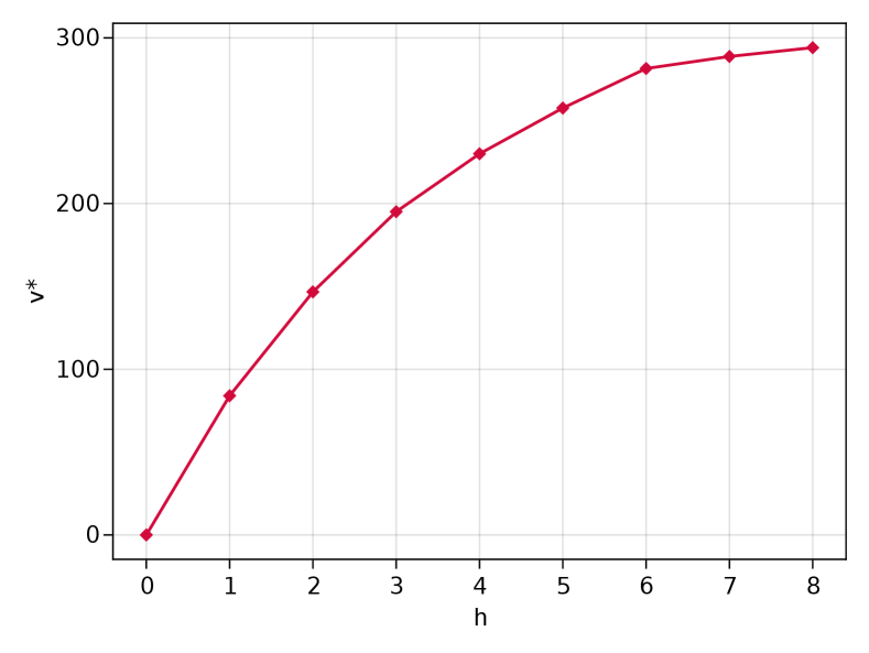
Let us examine a fictional admissions market consisting of schools. The school data, along with the optimal solutions for each , appear in Table 1.
Below are shown the first several iterations of Algorithm 1. The values of , , and their product are recorded only for the schools remaining in . , where , denotes the entrywise product of and . The school added at each iteration, underlined, is the one whose -value is greatest.
| Iteration 1: | |||||
| Iteration 2: | |||||
| Iteration 3: | |||||
| Iteration 8: | |||||
The output of the algorithm is , and the optimal -portfolio consists of its first entries. The “priority” column of Table 1 shows the inverse permutation of , which is the minimum value of for which the school is included in the optimal portfolio. Figure 1 shows the value of the optimal portfolio as a function of . The concave shape of the plot suggests the result of Theorem 5.
| Index | School | Admit prob. | Utility | Priority | |
|---|---|---|---|---|---|
| 1 | Mercury University | 0.39 | 200 | 4 | 230.0 |
| 2 | Venus University | 0.33 | 250 | 2 | 146.7 |
| 3 | Mars University | 0.24 | 300 | 6 | 281.5 |
| 4 | Jupiter University | 0.24 | 350 | 1 | 84.0 |
| 5 | Saturn University | 0.05 | 400 | 7 | 288.8 |
| 6 | Uranus University | 0.03 | 450 | 8 | 294.1 |
| 7 | Neptune University | 0.10 | 500 | 5 | 257.7 |
| 8 | Pluto College | 0.12 | 550 | 3 | 195.1 |
4 Heterogeneous application costs
Now we turn to the more general problem in which the constant represents the cost of applying to and the student, whom we now call Ellis, has a budget of to spend on college applications. Applying Lemma 1, we assume throughout.
Problem 2엘리스의 문제. (Ellis’s problem).
Ellis’s optimal college application portfolio is given by the solution to the following combinatorial optimization problem.
| (20) | ||||
In this section, we show that this problem is NP-complete, then provide four algorithmic solutions: an exact branch-and-bound routine, an exact dynamic program, a fully polynomial-time approximation scheme (FPTAS), and a simulated-annealing heuristic.
4.1 NP-completeness
The optima for Ellis’s problem are not necessarily nested, nor is the number of schools in the optimal portfolio necessarily increasing in . For example, if , , and , then it is evident that the optimal portfolio for is while that for is . In fact, Ellis’s problem is NP-complete, as we will show by a transformation from the binary knapsack problem, which is known to be NP-complete (Garey and Johnson 1979, § 3.2.1).
Problem 3배낭 문제의 결정 형태. (Decision form of knapsack problem).
An instance consists of a set of objects, utility values and weight for each , and target utility and knapsack capacity . The instance is called a yes-instance if and only if there exists a set having and .
Problem 4엘리스 문제의 결정 형태. (Decision form of Ellis’s problem).
An instance consists of an instance of Ellis’s problem and a target valuation . The instance is called a yes-instance if and only if there exists a portfolio having and .
Theorem 6.
The decision form of Ellis’s problem is NP-complete.
Proof.
It is obvious that the problem is in NP.
Consider an instance of the knapsack problem, and we will construct an instance of Problem 4 that is a yes-instance if and only if the corresponding knapsack instance is a yes-instance. Without loss of generality, we may assume that the objects in are indexed in increasing order of , that each , and that each .
Let and , and construct an instance of Ellis’s problem with , , all , and each . Clearly, is feasible for Ellis’s problem if and only if it is feasible for the knapsack instance. Now, we observe that for any nonempty ,
| (21) | ||||
This means that the utility of an application portfolio in the corresponding knapsack instance is the smallest integer greater than . That is, if and only if . Taking completes the transformation and concludes the proof. ∎
An intuitive extension of the greedy algorithm for Alma’s problem is to iteratively add to the school for which is largest. But the construction above shows that the objective function of Ellis’s problem can approximate that of a knapsack problem with arbitrary precision. Therefore, in pathological examples such as the following, the greedy algorithm can achieve an arbitrarily small approximation ratio.
Example 3.
Let , , , and . Then the greedy approximation algorithm produces the clearly suboptimal solution .
We might expect to obtain a better approximate solution to Ellis’s problem by solving the following knapsack problem (nevermind that it is NP-complete) as a surrogate.
| (22) |
However, upon inspection, this solution merely generalizes the naïve algorithm for Alma’s problem (Definition 3). In Ellis’s problem, because the number of schools in the optimal portfolio can be as large as , the knapsack solution’s approximation coefficient is by analogy with (13). A tight example is as follows.
Example 4.
Consider the following instance of Ellis’s problem, where .
The feasible solutions and each have , and thus the knapsack algorithm can choose with . But the optimal solution is with .
In summary, neither a greedy algorithm nor a knapsack-based algorithm solves Ellis’s problem to optimality.
4.2 Branch-and-bound algorithm
A traditional approach to integer optimization problems is the branch-and-bound framework, which generates subproblems in which the values of one or more decision variables are fixed and uses an upper bound on the objective function to exclude, or fathom, branches of the decision tree that cannot yield a solution better than the best solution on hand (Martello and Toth 1990; Kellerer et al. 2004). In this subsection, we present an integer formulation of Ellis’s problem and a linear program (LP) that bounds the objective value from above. We tighten the LP bound for specific subproblems by reusing the conditional transformation of the -values from Algorithm 1. A branch-and-bound routine emerges naturally from these ingredients.
To begin, let us characterize the portfolio as the binary vector , where if and only if . Then it is not difficult to see that Ellis’s problem is equivalent to the following integer nonlinear program.
Problem 5엘리스의 문제를 위한 비선형 정수 계획. (Integer NLP for Ellis’s problem).
| (23) | ||||
Since the product in does not exceed one, the following LP relaxation is an upper bound on the valuation of the optimal portfolio.
Problem 6엘리스의 문제를 위한 선형 완화 문제. (LP relaxation for Ellis’s problem).
| (24) | ||||
Problem 6 is a continuous knapsack problem, which is easily solved in -time by a greedy algorithm (Dantzig 1957). Balas and Zemel (1980, § 2) provide an algorithm.
In our branch-and-bound framework, a node is characterized by a three-way partition of schools satisfying . consists of schools that are “in” the application portfolio (), consists of those that are “out” (), and consists of those that are “negotiable.” The choice of partition induces a pair of subproblems. The first subproblem is an instance of Problem 5, namely
| (25) | ||||
The second is the corresponding instance of Problem 6:
| (26) | ||||
In both subproblems, denotes the residual budget. The parameters and are obtained by iteratively applying the transformation (7) to the schools in . For each , we increment by the current value of , eliminate from the market, and update the remaining -values using (7). (An example is given below.)
Given a node , its children are generated as follows. Every node has two, one, or zero children. In the typical case, we select a school for which and generate one child by moving to , and another child by moving it to . Equivalently, we set in one child and in the other. In principle, any school can be chosen for , but as a greedy heuristic, we choose the school for which the ratio is highest. Notice that this method of generating children ensures that each node’s -set differs from its parent’s by at most a single school, so the constant and transformed -values for the new node can be obtained by a single application of (7).
There are two atypical cases. First, if every school in has , then there is no school that can be added to in a feasible portfolio, and the optimal portfolio on this branch is itself. In this case, we generate only one child by moving all the schools from to . Second, if , then the node has zero children, and as no further branching is possible, the node is called a leaf.
Example 5.
Consider a market in which , , , and , and the node . Let us compute the two subproblems associated with and identify its children. To compute the subproblems, we first simply disregard . Next, to eliminate , we apply (7) to to obtain and . We eliminate by again applying (7) to to obtain and . Finally, . Now problems (25) and (26) are easily obtained by substitution.
Since at least one of the schools in has , has two children. Applying the node-generation rule, has the highest -ratio, so the children are and .
To implement the branch-and-bound algorithm, we represent the set of candidate nodes—namely, nonleaf nodes whose children have not yet been generated—by . Each time a node is generated, we record the values and , the optimal objective value of the LP relaxation (26). Because is a feasible portfolio, is a lower bound on the optimal objective value. Moreover, by the argument given in the proof of Theorem 3, the objective function of (25) is identical to the function . This means that is an upper bound on the valuation of any portfolio that contains as a subset and does not include any school in , and hence on the valuation of any portfolio on this branch. Therefore, if upon generating a new node , we discover that its objective value is greater than for some other node , then we can disregard and all its descendants.
The algorithm is initialized by populating with the root node . At each iteration, it selects the node having the highest -value, generates its children, and removes from the candidate set. Next, the children of are inspected and added to the tree. If one of the children yields a new optimal solution, then we mark it as the best candidate and fathom any nodes for which . When no nodes remain in the candidate set, the algorithm has explored every branch, so it returns the best candidate and terminates.
Theorem 7알고리즘 2의 타당성. (Validity of Algorithm 2).
Algorithm 2 produces an optimal application portfolio for Ellis’s problem.
Proof.
Because an optimal solution exists among the leaves of the tree, the discussion above implies that as long as the algorithm terminates, it returns an optimal solution.
To show that the algorithm does not cycle, it suffices to show that no node is generated twice. Suppose not: that two distinct nodes and share the same partition . Trace each node’s lineage up the tree and let denote the first node at which the lineages meet. must have two children, or else its sole child is a common ancestor of and , and one of these children, say , must be an ancestor of while the other, say , is an ancestor of . Write and . By the node-generation rule, there is a school in , and the -set (respectively, -set) for any descendant of (respectively, ) is a superset of (respectively, ). Therefore, , meaning that is not a partition of , a contradiction. ∎
The branch-and-bound algorithm is an interesting benchmark, but as a kind of enumeration algorithm, its computation time grows rapidly in the problem size, and unlike the approximation scheme we propose later on, there is no guaranteed bound on the approximation error after a fixed number of iterations. Moreover, when there are many schools in , the LP upper bound may be much higher than . This means that significant fathoming operations do not occur until the algorithm has explored deep into the tree, at which point the bulk of the computational effort has already been exhausted. In our numerical experiments, Algorithm 2 was ineffective on instances larger than about schools, and therefore it does not represent a significant improvement over naïve enumeration. We speculate that the algorithm can be improved by incorporating cover inequalities (Wolsey 1998, § 9.3).
4.3 Pseudopolynomial-time dynamic program
In this subsection, we assume, with a small loss of generality, that for and , and provide an algorithmic solution to Ellis’s problem that runs in -time. The algorithm resembles a familiar dynamic programming algorithm for the binary knapsack problem (Dantzig 1957; Wikipedia, s.v. “Knapsack problem”). Because we cannot assume that (as was the case in Alma’s problem), this represents a pseudopolynomial-time solution (Garey and Johnson 1979, § 4.2). However, it is quite effective for typical college-application instances in which the application costs are small integers.
For and , let denote the optimal portfolio using only the schools and costing no more than , and let . It is clear that if or , then and . For convenience, we also define for all .
For the remaining indices, either contains or not. If it does not contain , then . On the other hand, if contains , then its valuation is . This requires that make optimal use of the remaining budget over the remaining schools; that is, . From these observations, we obtain the following Bellman equation for and :
| (27) |
with the convention that . The corresponding optimal portfolios are computed by observing that contains if and only if . The optimal solution is given by . The algorithm below performs these computations and outputs the optimal portfolio .
Theorem 8알고리즘 3의 타당성. (Validity of Algorithm 3).
Algorithm 3 produces an optimal application portfolio for Ellis’s problem in -time.
Proof.
Optimality follows from the foregoing discussion. Sorting is . The bottleneck step is the creation of the lookup table for in line 3. Each entry is generated in unit time, and the size of the table is . ∎
4.4 Fully polynomial-time approximation scheme
As with the knapsack problem, Ellis’s problem admits a complementary dynamic program that iterates on the value of the cheapest portfolio instead of on the cost of the most valuable portfolio. We will use this algorithm as the basis for an FPTAS for Ellis’s problem that uses -time and -space.
We will represent approximate portfolio valuations using a fixed-point decimal with a precision of , where is the number of digits to retain after the decimal point. Let denote the value of rounded down to its nearest fixed-point representation. Since is an upper bound on the valuation of any portfolio, and since we will ensure that each fixed-point approximation is an underestimate of the portfolio’s true valuation, the set of possible valuations possible in the fixed-point framework is finite:
| (28) |
Then .
For the remainder of this subsection, unless otherwise specified, the word valuation refers to a portfolio’s valuation within the fixed-point framework, with the understanding that this is an approximation. We will account for the approximation error below when we prove the dynamic program’s validity.
For integers and , let denote the least expensive portfolio that uses only schools and has valuation at least , if such a portfolio exists. Denote its cost by , where if does not exist. It is clear that if , then and , and that if and , then . For the remaining indices (where ), we claim that
| (29) | ||||
| (30) |
In the case, any feasible portfolio must be composed of schools with utility less than , and therefore its valuation can not equal , meaning that is undefined. In the case, the first argument to says simply that omitting and choosing is a permissible choice for . If, on the other hand, , then
| (31) |
Therefore, the subportfolio must have a valuation of at least , where satisfies . When , the solution to this equation is . By rounding this value down, we ensure that the true valuation of is at least . When and , the singleton has , so
| (32) |
Defining in this case ensures that as required.
Once has been calculated at each index, the associated portfolio can be found by applying the observation that contains if and only if . Then an approximate solution to Ellis’s problem is obtained by computing the largest achievable objective value and corresponding portfolio.
Theorem 9알고리즘 4의 타당성. (Validity of Algorithm 4).
Algorithm 4 produces a -optimal application portfolio for Ellis’s problem in -time.
Proof.
(Optimality.) Let denote the output of Algorithm 4 and the true optimum. We know that , and because each singleton portfolio is feasible, must be more valuable than the average singleton portfolio; that is, .
Because is rounded down in the recursion relation defined by (29) and (30), if , then the true value of may exceed the fixed-point valuation of , but not by more than . This error accumulates additively with each school added to , but the number of additions is at most . Therefore, where denotes the fixed-point valuation of recorded in line 4 of the algorithm, .
We can define analogously as the fixed-point valuation of when its elements are added in index order and its valuation is updated and rounded down to the nearest multiple of at each addition in accordance with (31). By the same logic, . The optimality of in the fixed-point environment implies that .
Applying these observations, we have
| (33) |
which establishes the approximation bound.
(Computation time.) The bottleneck step is the creation of the lookup table in line 4, whose size is . Since
| (34) |
is , the time complexity is as promised. ∎
Since its time complexity is polynomial in and , Algorithm 4 is an FPTAS for Ellis’s problem (Vazirani 2001).
4.5 Simulated annealing heuristic
Simulated annealing is a popular local-search heuristic for nonconvex optimization problems. Because of their inherent randomness, simulated-annealing algorithms offer no accuracy guarantee; however, they are easy to implement, computationally inexpensive, and often produce solutions with a small optimality gap. In this section, we present a simulated-annealing algorithm for Ellis’s problem. It is patterned on the procedure for integer programs outlined by Wolsey (1998, § 12.3.2).
To generate an initial solution, our algorithm adopts the greedy heuristic of adding schools in descending order by until the budget is exhausted. While Example 3 shows that the approximation coefficient of this solution can be arbitrarily small, in typical instances, it is much higher. Next, given a candidate solution , we generate a neighbor by copying , adding schools to until it becomes infeasible, then removing elements of from until feasibility is restored. If , then the candidate solution is updated to equal the neighbor; if not, then the candidate solution is updated with probability , where is a temperature parameter. This is repeated times, and the algorithm returns the best observed.
Proposition 2.
The computation time of Algorithm 5 is .
In our numerical experiments, the output of Algorithm 5 was typically quite close to the optimum.
5 Numerical experiments
In this section, we present the results of numerical experiments designed to test the practical efficacy of the algorithms derived above.
5.1 Implementation notes
We chose to implement our algorithms in the Julia language (v1.8.0b1) because its system of parametric data types allows the compiler to optimize for differential cases such as when the -values are integers or floating-point numbers. Julia also offers convenient macros for parallel computing, which enabled us to solve more and larger problems in the benchmark (Bezanson et al. 2017). We made extensive use of the DataStructures.jl package (v0.18.11, github.com/JuliaCollections). The code is available at github.com/maxkapur/OptimalApplication.
The dynamic programs, namely Algorithms 3 and 4, were implemented using recursive functions and dictionary memoization, as described in Cormen et al. (1990, § 16.6). Our implementation of Algorithm 4 also differed from that described in Subsection 4.4 in that we represented portfolio valuations in binary rather than decimal, with the definitions of and modified accordingly, and instead of fixed-point numbers, we worked in integers by multiplying each element of by . These modifications yield a substantial performance improvement without changing the fundamental algorithm design or complexity analysis.
5.2 Experimental procedure
We conducted three numerical experiments. Experiments 1 and 2 evaluate the computation times of our algorithms for Alma’s problem and Ellis’s problem, respectively. Experiment 3 investigates the empirical accuracy of the simulated-annealing heuristic as compared to an exact algorithm.
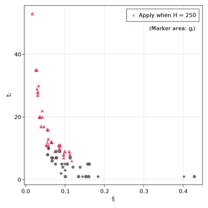
To generate synthetic markets, we drew the -values independently from an exponential distribution with a scale parameter of ten and rounded up to the nearest integer. To achieve partial negative correlation between and , we then set , where is drawn uniformly from the interval . In Experiment 1, which concerns Alma’s problem, we set . In Experiments 2 and 3, which concern Ellis’s problem, each is drawn uniformly from the set and we set . This cost distribution resembles real-world college application fees, which are often multiples of $10 between $50 and $100. A typical instance is shown in Figure 2.
The experimental variables in Experiments 1 and 2 were the market size , the choice of algorithm, and (for Algorithm 4) the tolerance . For each combination of the experimental variables, we generated 50 markets, and the optimal portfolio was computed three times, with the fastest of the three repetitions recorded as the computation time. We then report the mean and standard deviation across the 50 markets. Therefore, each cell of each table below represents a statistic over 150 computations. Where applicable, we do not count the time required to sort the entries of . As the simulated-annealing heuristic’s computation time is negligible, it was excluded from Experiment 2.
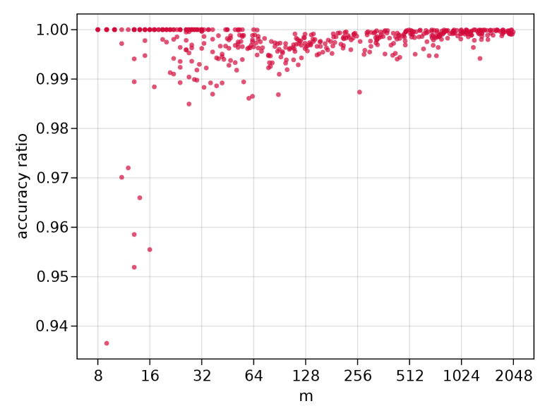
In Experiment 3, we generated 500 markets with sizes varying uniformly in the logarithm between and . For each market, we computed a heuristic solution using Algorithm 5 and an exact solution using Algorithm 3 and calculated the optimality ratio. We chose to use iterations in the simulated-annealing algorithm, and the temperature parameters and were selected by a preliminary grid search.
5.3 Summary of results
Experiment 1 compared the performance of Algorithm 1 for homogeneous-cost markets of various sizes when the set of candidate schools is stored as a list and as a binary max heap ordered by the -values. The results appear in Table 2. Our results indicate that the list implementation is faster.
In Experiment 2, we turned to the general problem, and compared the performance of the exact algorithms (Algorithms 2 and 3) and the approximation scheme (Algorithm 4) at tolerances 0.5 and 0.05. The results, which appear in Table 3, broadly agree with the time complexity analyses presented above. The branch-and-bound algorithm proved impractical for even medium-sized instances. Overall, we found the exact dynamic program to be the fastest algorithm, while the FPTAS was rather slow, a result that echoes the results of computational studies on knapsack problems (Martello and Toth 1990, § 2.10). The strong performance of Algorithm 3 is partly attributable to the structure of our synthetic instances, in which application costs are small integers and is proportional in expectation to , meaning the expected computation time is . However, the relative advantage of Algorithm 3 may be even more pronounced in real college-application instances because the typical student’s application budget accommodates at most a dozen or so schools and is constant in .
The results of Experiment 3, which evaluated the performance of the simulated-annealing heuristic in our synthetic instances, are plotted in Figure 3. In the every instance, the heuristic found a solution within 10 percent of optimality, and in the vast majority of instances, it was within 2 percent of optimality. The heuristic performs most poorly in small markets of size , but as exact algorithms are tractable at this scale, this result presents no cause for concern.
|
|
|
||||||||
|---|---|---|---|---|---|---|---|---|---|---|
| 16 | 0.00 | (0.00) | 0.01 | (0.00) | ||||||
| 64 | 0.01 | (0.00) | 0.08 | (0.02) | ||||||
| 256 | 0.06 | (0.00) | 0.96 | (0.26) | ||||||
| 1024 | 0.82 | (0.03) | 14.27 | (2.28) | ||||||
| 4096 | 12.87 | (0.71) | 230.77 | (18.75) | ||||||
| 16384 | 199.48 | (1.77) | 3999.19 | (283.48) | ||||||
|
|
|
|
|
||||||||||||||
|---|---|---|---|---|---|---|---|---|---|---|---|---|---|---|---|---|---|---|
| 8 | 0.02 | (0.01) | 0.01 | (0.00) | 0.05 | (0.01) | 0.16 | (0.04) | ||||||||||
| 16 | 0.10 | (0.04) | 0.07 | (0.02) | 0.39 | (0.10) | 2.59 | (0.62) | ||||||||||
| 32 | 12.43 | (9.88) | 0.29 | (0.05) | 2.15 | (0.29) | 33.07 | (10.72) | ||||||||||
| 64 | — | (—) | 1.24 | (0.16) | 13.24 | (2.22) | 339.64 | (100.38) | ||||||||||
| 128 | — | (—) | 6.20 | (0.64) | 79.92 | (20.18) | 2042.63 | (749.71) | ||||||||||
| 256 | — | (—) | 30.63 | (2.28) | 818.50 | (632.98) | 18949.50 | (3533.88) | ||||||||||
6 Conclusion and ideas for future research
This study has introduced a novel combinatorial optimization problem that we call the college application problem. It can be viewed as a kind of asset allocation or knapsack problem with a submodular objective. We showed that the special case in which colleges have identical application costs can be solved in polynomial time by a greedy algorithm because the optimal solutions are nested in the budget constraint. The general problem is NP-complete. We provided four solution algorithms. The strongest from a theoretical standpoint is an FPTAS that produces a -approximate solution in -time. On the other hand, for typical college-application instances, the dynamic program based on application expenditures is both easier to implement and substantially more time efficient. A heuristic simulated-annealing algorithm also exhibited strong empirical performance in our computational study. The algorithms discussed in this paper are summarized in Table 4.
| Algorithm | Reference | Problem | Restrictions | Exactness | Computation time | |||
|---|---|---|---|---|---|---|---|---|
\addstackgap[.5]
|
Definition 3 |
|
None | -opt. | ||||
| \addstackgap[.5] Greedy | Algorithm 1 |
|
None | Exact | ||||
\addstackgap[.5]
|
Algorithm 2 | General | None | Exact | ||||
| \addstackgap[.5] Costs DP | Algorithm 3 | General | integer | Exact | ||||
| \addstackgap[.5] FPTAS | Algorithm 4 | General | None | -opt. | ||||
\addstackgap[.5]
|
Algorithm 5 | General | None | -opt. |
Three extensions of this problem appear amenable to future study.
6.1 Explicit treatment of risk aversion
The familiar Markowitz portfolio optimization model includes an explicit risk-aversion term, whereas our model has settled for an implicit treatment of risk, namely the tradeoff between selective schools and safety schools inherent in the maximax objective function. However, it is possible to augment the objective function to incorporate a variance penalty as follows:
| (35) | ||||
where . Since the first term is itself a portfolio valuation function, and the second is a monotonic transformation of one, we speculate that one of the algorithms given above could be used as a subroutine to trace out the efficient frontier by maximizing subject to the budget constraint and for various values of .
A parametric treatment of risk aversion may align our model more closely to real-world applicant behavior. Conventional wisdom asserts that the best college application strategy combines reach, target, and safety schools in roughly equal proportion (Jeon 2015). When the application budget is small relative to the size of the admissions market, our algorithms recommend a similar approach (see the example of Subsection 3.5). However, inspecting equation (7), which discounts school utility parameters to reflect their marginal value relative to the schools already in the portfolio, reveals that low-utility schools are penalized more harshly than high utility schools in the marginal analysis. Consequentially, as the application budget grows, the optimal portfolio in our model tends to favor reach schools over safety schools. (See Figure 2 for a clear illustration of this phenomenon.)
A potential application of our model is an econometric study that estimates students’ perceptions of college quality () from their observed application behavior () under the assumption of utility maximization. Empirical research indicates that heterogeneous risk aversion is a significant source of variation in human decision-making, especially in the domains of educational choice and employment search (Kahneman 2011; Hartlaub and Schneider 2012; van Huizen and Alessie 2019). Therefore, an endogenous risk-aversion parameter would greatly enhance our model’s explanatory power in the econometric setting.
6.2 Signaling strategies
Another direction of further research with immediate application in college admissions is to incorporate additional signaling strategies into the problem. In the Korean admissions process, the online application form contains three multiple-choice fields, labeled ga, na, and da for the first three letters of the Korean alphabet, which students use to indicate the colleges to which they wish to apply. Most schools appear only in one or two of the three fields. Therefore, students are restricted not only in the number of applications they can submit, but in the combinations of schools that may coincide in a feasible application portfolio. From a portfolio optimization perspective, this is a diversification constraint, because its primary purpose is to prevent students from applying only to top-tier schools. However, in addition to overall selectivity, the three fields also indicate different evaluation schemes: The ga and na customarily indicate the applicant’s first and second choice, and applications filed under these fields are evaluated with greater emphasis on standardized-test scores than those filed under the da field. Some colleges appear in multiple fields and run two parallel admissions processes, each with different evaluation criteria. Therefore, if a student recognizes that she has a comparative advantage in (for example) her interview skills, she may increase her chances of admission to a competitive school by applying under the da field. The optimal application strategy in this context can be quite subtle, and it is a subject of perennial debate on Korean social networks.
An analogous feature of the American college admissions process is known as early decision, in which at the moment of application, a student commits to enrolling in a college if admitted. In principle, students who apply with early decision may obtain a better chance of admission by signaling their eagerness to attend, but doing so weakens the college’s incentive to entice the student with discretionary financial aid, altering the utility calculus.
In the integer formulation of the college application problem (Problem 5), a natural way to model these signaling strategies without introducing too much complexity is to split each into and . The binary decision variables are if the student applies to with high priority (that is, in the ga or na field or with early decision) and if applying with low priority (that is, in the da field or without early decision). Now, assuming that the differential admission probabilities and and utilities and are known, adding the logical constraints
| (36) |
completes the formulation. These are knapsack constraints; therefore, the submodular maximization algorithm of Kulik et al. (2013) can be used to obtain a -approximate solution for this problem. When the budget constraint is a cardinality constraint (as in Alma’s problem), we note that adding these constraints yields a matroidal solution set, and Calinescu et al. (2011)’s algorithm yields an alternative solution, which has the same approximation coefficient of .
6.3 Memory-efficient dynamic programs
Our numerical experiments suggest that the performance of the dynamic programming algorithms is bottlenecked by not computation time, but memory usage. Reducing these algorithms’ storage requirements would enable us to solve considerably larger problems.
Abstractly speaking, Algorithms 3 and 4 are two-dimensional dynamic programs that represent the optimal solution by . Here is the number of decision variables, is a constraint parameter, and is the optimal objective value achievable using the first decision variables when the constraint parameter is . The algorithm iterates on a recursion relation that expresses as a function of and for some . (In Algorithm 3, is the maximal portfolio valuation, , and ; in Algorithm 4, is the minimal application expenditures, , and .)
When such a dynamic program is implemented using a lookup table or dictionary memoization, producing the optimal solution requires -time and -space. Kellerer et al. (2004, § 3.3) provide a technique for transforming the dynamic program into a divide-and-conquer algorithm that produces the optimal solution in -time and -space, a significant improvement. However, their technique requires the objective function to be additively separable in a certain sense that appears difficult to conform to the college application problem.
Appendix A Appendix
A.1 Elementary proof of Theorem 5
Proof.
We will prove the equivalent expression . Applying Theorem 3, we write and . If , then
| (37) | ||||
The first inequality follows from the optimality of , while the second follows from the fact that adding to can only increase its valuation.
If , then the steps are analogous:
| (38) | ||||
| (39) | ||||
References
Acharya, Mohan S., Asfia Armaan, and Aneeta S. Antony. 2019. “A Comparison of Regression Models for Prediction of Graduate Admissions.” In Second International Conference on Computational Intelligence in Data Science. https://doi.org/10.1109/ICCIDS.2019.8862140.
Badanidiyuru, Ashwinkumar and Jan Vondrák. 2014. “Fast Algorithms for Maximizing Submodular Functions.” In Proceedings of the 2014 Annual ACM–SIAM Symposium on Discrete Algorithms, 1497–1514. https://doi.org/10.1137/1.9781611973402.110.
Balas, Egon and Eitan Zemel. 1980. “An Algorithm for Large Zero-One Knapsack Problems.” Operations Research 28 (5): 1130–54. https://doi.org/10.1287/opre.28.5.1130.
Bezanson, Jeff, Alan Edelman, Stefan Karpinski, and Viral B. Shah. 2017. “Julia: A Fresh Approach to Numerical Computing.” SIAM Review 59: 65–98. https://doi.org/10.1137/141000671.
Blum, Manuel, Robert W. Floyd, Vaughan Pratt, Ronald L. Rivest, and Robert E. Tarjan. 1973. “Time Bounds for Selection.” Journal of Computer and System Sciences 7 (4): 448–61. https://doi.org/10.1016/S0022-0000(73)80033-9.
Calinescu, Gruia, Chandra Chekuri, Martin Pál, and Jan Vondrák. 2011. “Maximizing a Monotone Submodular Function Subject to a Matroid Constraint.” SIAM Journal on Computing 40 (6): 1740–66. https://doi.org/10.1137/080733991.
Carraway, Robert, Robert Schmidt, and Lawrence Weatherford. 1993. “An Algorithm for Maximizing Target Achievement in the Stochastic Knapsack Problem with Normal Returns.” Naval Research Logistics 40 (2): 161–73. https://doi.org/10.1002/nav.3220400203.
Cormen, Thomas, Charles Leiserson, and Ronald Rivest. 1990. Introduction to Algorithms. Cambridge, MA: The MIT Press.
Dantzig, George B. 1957. “Discrete-Variable Extremum Problems.” Operations Research 5 (2): 266–88.
Dean, Brian, Michel Goemans, and Jan Vondrák. 2008. “Approximating the Stochastic Knapsack Problem: The Benefit of Adaptivity.” Mathematics of Operations Research 33 (4): 945–64. https://doi.org/10.1287/moor.1080.0330.
Kellerer, Hans, Ulrich Pferschy, and David Pisinger. 2004. Knapsack Problems. Berlin: Springer.
Kulik, Ariel, Hadas Shachnai, and Tami Tamir. 2013. “Approximations for Monotone and Nonmonotone Submodular Maximization with Knapsack Constraints.” Mathematics of Operations Research 38 (4): 729–39. https://doi.org/10.1287/moor.2013.0592.
Jeon, Minhee. 2015. “[College application strategy] Six chances total…divide applications across reach, target, and safety schools” (in Korean). Jungang Ilbo, Aug. 26. https://www.joongang.co.kr/article/18524069.
Fisher, Marshall, George Nemhauser, and Laurence Wolsey. 1978. “An Analysis of Approximations for Maximizing Submodular Set Functions—I.” Mathematical Programming 14: 265–94.
Fu, Chao. 2014. “Equilibrium Tuition, Applications, Admissions, and Enrollment in the College Market.” Journal of Political Economy 122 (2): 225–81. https://doi.org/10.1086/675503.
Garey, Michael and David Johnson. 1979. Computers and Intractability: A Guide to the Theory of NP-Completeness. New York: W. H. Freeman and Company.
Hartlaub, Vanessa and Thorsten Schneider. 2012. “Educational Choice and Risk Aversion: How Important Is Structural vs. Individual Risk Aversion?” SOEPpapers on Multidisciplinary Panel Data Research, no. 433. https://www.diw.de/documents/publikationen/73/diw_01.c.394455.de/diw_sp0433.pdf.
Kahneman, Daniel. 2011. Thinking, Fast and Slow. New York: Macmillan.
Markowitz, Harry. 1952. “Portfolio Selection.” The Journal of Finance 7 (1): 77–91. https://www.jstor.org/stable/2975974.
Martello, Silvano and Paolo Toth. 1990. Knapsack Problems: Algorithms and Computer Implementations. New York: John Wiley & Sons.
Meucci, Attilio. 2005. Risk and Asset Allocation. Berlin: Springer-Verlag, 2005.
Rozanov, Mark and Arie Tamir. 2020. “The Nestedness Property of the Convex Ordered Median Location Problem on a Tree.” Discrete Optimization 36: 100581. https://doi.org/10.1016/j.disopt.2020.100581.
Sklarow, Mark. 2018. State of the Profession 2018: The 10 Trends Reshaping Independent Educational Consulting. Technical report, Independent Educational Consultants Association. https://www.iecaonline.com/wp-content/uploads/2020/02/IECA-Current-Trends-2018.pdf.
Sniedovich, Moshe. 1980. “Preference Order Stochastic Knapsack Problems: Methodological Issues.” The Journal of the Operational Research Society 31 (11): 1025–32. https://www.jstor.org/stable/2581283.
Steinberg, E. and M. S. Parks. 1979. “A Preference Order Dynamic Program for a Knapsack Problem with Stochastic Rewards.” The Journal of the Operational Research Society 30 (2): 141–47. https://www.jstor.org/stable/3009295.
Van Huizen, Thomas and Rob Alessie. 2019. “Risk Aversion and Job Mobility.” Journal of Economic Behavior & Organization 164: 91–106. https://doi.org/10.1016/j.jebo.2019.01.021.
Vazirani, Vijay. 2001. Approximation Algorithms. Berlin: Springer.
Wolsey, Laurence. 1998. Integer Programming. New York: John Wiley & Sons.