This is the author accepted manuscript (AAM) of the following published article:
| DOI | https://doi.org/10.1088/1748-9326/ad27b9 |
|---|---|
| arXiv DOI | https://doi.org/10.48550/arXiv.2307.08909 |
| author(s) | Laurens P. Stoop, Karin van der Wiel, William Zappa, Arno Haverkamp, Ad J. Feelders, Machteld van den Broek |
| title | The Climatological Renewable Energy Deviation Index (credi) |
| publication date | February 2024 |
| journal | Enviromental Research Lettes |
| volume | 19 |
| page numbers | 034021 |
This AAM version corresponds to the author’s final version of the article, as accepted by the journal. However, it has not been copy-edited or formatted by the journal.
This AAM is deposited under a Creative Commons Attribution–ShareAlike (CC-BY-SA) license.
The Climatological Renewable Energy Deviation Index (credi)
Abstract
We propose an index to quantify and analyse the impact of climatological variability on the energy system at different timescales.
We define the Climatological Renewable Energy Deviation Index (credi) as the cumulative anomaly of a renewable resource with respect to its climate over a specific time period of interest.
For this we introduce the smooth, yet physical, hourly rolling window climatology that captures the expected hourly to yearly behaviour of renewable resources.
We analyse the presented index at decadal, annual and (sub-)seasonal timescales for a sample region and discuss scientific and practical implications.
credi is meant as an analytical tool for researchers and stakeholders to help them quantify, understand, and explain, the impact of energy-meteorological variability on future energy system.
Improved understanding translates to better assessments of how renewable resources, and the associated risks for energy security, may fare in current and future climatological settings.
The practical use of the index is in resource planning.
For example transmission system operators may be able to adjust short-term planning to reduce adequacy issues before they occur or combine the index with storyline event selection for improved assessments of climate change related risks.
Keywords: Resource droughts, Resource Adequacy, Renewable Energy Drought, Dunkelflaute, Wind Drought
1 Introduction
The energy system is changing. This is due to the increased deployment of renewable energy generators, like wind turbines and solar panels; changes in electricity demand, from increased use of heat pumps and electric vehicles; and climatic changes influencing the weather dependent parts of the system. It is crucial to understand the full dynamics of the (future) energy system, both for policy making and energy security reasons [1].
Knowing the impact of and link between the energy system and weather-related variability on daily to inter-annual and decadal timescales is vital for robust design and planning of future energy systems [2, 1, 3]. Meteorological variability leads to temporal variability. Not only in renewable energy production, but also in energy demand, changing the way energy systems have to be operated and controlled [1].
Energy system models are vital to capture the impact of this variability [4]. However, their complexity results in high computational burdens that grows exponentially with the simulation period [5, 6, 1, 7, 8]. Incorporating large climate datasets that capture energy-meteorological variability in operational hourly energy system models is thus, as of yet, unfeasible [9, 1, 7]. Even so, understanding the scale of this variability, can aid system operators in their task to ensure both short- and long-term energy security [1, 7, 10]. Therefore, alternative approaches are needed to assess energy-meteorological variability [1, 11]. While a number of methods exists to model and/or select challenging high impact events using basic statistical principles [[, e.g.]]vanderwiel2019extreme,Ohlendorf2020,OteroFelipe2021,stoop2021detection,vanderMost2022,Boston2022,Hu2023,Allen2023, we aim to define a physics based and intuitive to understand metric to quantify energy-meteorological variability across timescales.
In developing this metric, we were inspired by the hydrological sciences. For drought monitoring, a number of indices have proven useful for both scientific assessment and operational use. These drought indices, such as the Climatological Water Balance [[, CWB;]]gleick1985regional,Gleick1986, the Standardised Precipitation Index [[, SPI;]]mckee1993, and the Standardised Precipitation-Evapotranspiration Index [[, SPEI;]]VicenteSerrano2010), are based on precipitation deficits (anomaly of precipitation, or anomaly of the difference between potential evapotranspiration and precipitation) and are used to assess the temporal development of dry or wet periods. Furthermore, they have been used to assess the influence of inter-annual to multi-decadal variability, and of climate change on the temporal variability of hydrological drought [[, e.g.]]Quiring2009,Stagge2015,Cammalleri2021,vanderWiel2022. As [18] showed, some aspects of these indices and their use in assessing hydrological variability can be transferred to the energy-meteorological domain. However, where [18] developed direct analogues of the SPI and SPEI metrics using probabilistic descriptions, we took inspiration from aspects of these metrics, their use in operational applications, and combined this with the need for physically grounded storylines in energy system operation.
We define the Climatological Renewable Energy Deviation Index (credi) as the cumulative anomaly of a renewable resource with respect to its climate over a specific time period of interest (Figure 1). Given this definition, this study addresses the following considerations: (a) how do you define the climatic behaviour of a highly variable renewable resource, like wind or solar? and (b) how do you analyse the credi score at different timescales; like (sub-)seasonal, annual, or multi-decadal?

The paper is structured as follows. In Section 2, we define the hourly rolling window climate and the index. In Section 3, we indicate the data used. In Section 4, we analyse the index at different timescales and discuss the best starting point. In the Section 5 we discuss our definition of the index. Finally, in Section 6, a synthesis of our findings is presented and potential use cases in research and/or operational application are outlined. Supporting Information (SI) with additional figures and observational analysis is available online.
2 Definition of the climatic characterisation and index
Within the atmospheric sciences the climate of a region is defined as the statistical-mean weather conditions prevailing in that region [27]. The [[, WMO;]]wmo2017normals has a standardised method for calculation of the climatological normals, which comes down to calculating monthly or daily mean values over a 30-year period. The climate, or mean expected behaviour, of renewable resources could be defined similarly. However, monthly or daily climatological values are not suitable due to the highly variable nature of renewable resources like wind and solar energy, and the need to balance the power grid at shorter timescales.
We can distinguish four relevant timescales that cover the main modes of energy-meteorological variability. Namely:
-
1.
annual to decadal timescales: variability caused by interactions in the coupled ocean-atmosphere-system, e.g. modes of variability like the El-Niño-Southern Oscillation [[, ENSO;]]ipcc6_wg1_variability or the North Atlantic Oscillation [[, NAO;]]Wanner2001,
-
2.
seasonal timescale: variability caused by the revolution of the Earth around the Sun and the directly related variation of the solar declination angle,
-
3.
sub-seasonal timescale: variability caused by the cumulative interplay at various timescales, associated with the passing of weather systems and the changes in their persistence and occurrence,
-
4.
daily timescale: variability caused by the revolution of the Earth around its axis, and the directly related times of sunrise, sunset, and the solar elevation angle.
When studying the generation potential of wind or solar, all these timescales of variability should be considered.
2.1 A climatology of renewable resources and the use of hourly rolling windows
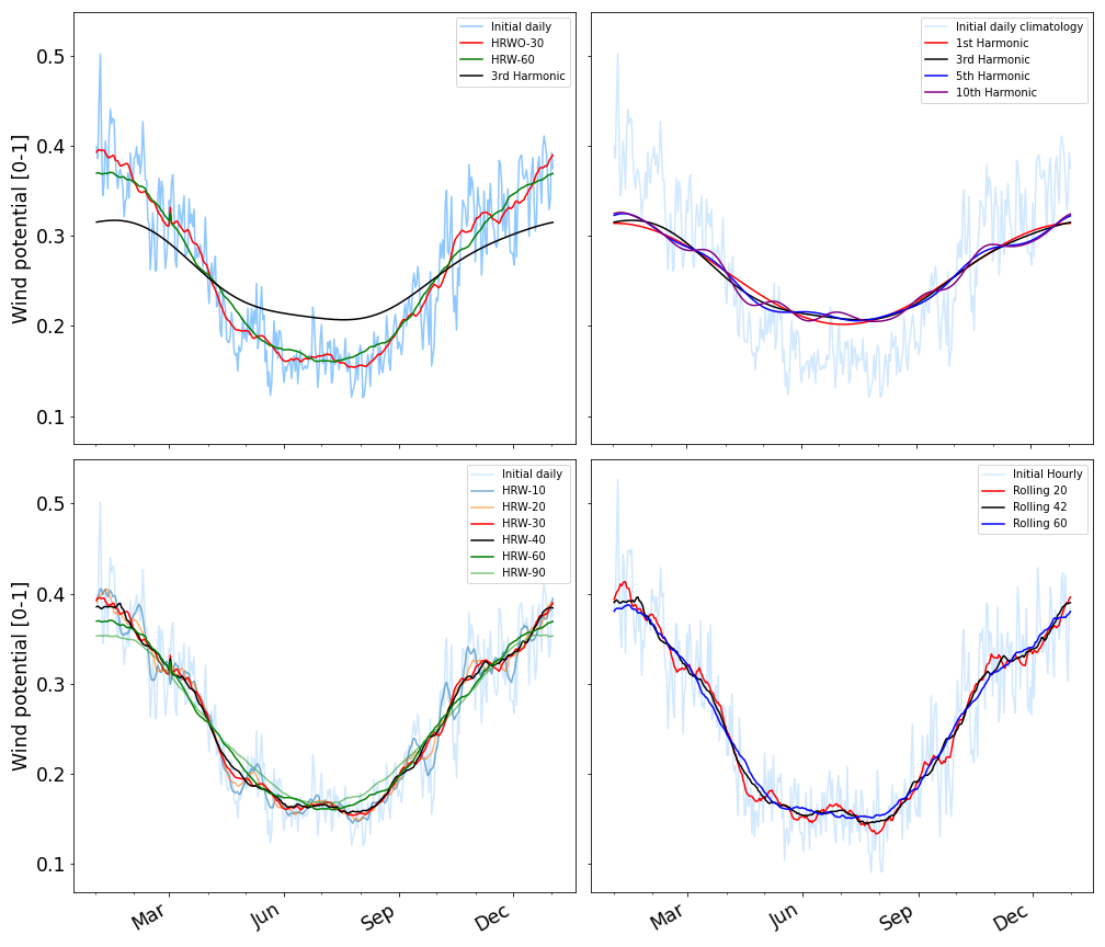
The highly variable nature of the wind and solar resources makes that a straightforward 30-year daily mean does not result in a useful definition of their climate (see SI Section A). The same holds for an initial estimate by averaging each ordinal hour over 30 years (Figure 2a,c). Though this simple average-based climatology does capture the mean expected behaviour on annual timescales, the random fluctuations from day-to-day and hour-to-hour cannot be explained by physical processes in this climatological definition. To remove these random fluctuations more data would be needed to obtain the desired, physical, smooth , but physical, climatology. However, considering a period longer than 30-years is ineffective, as climate change would start to influence the result[28]. Applying a simple running mean to this simple average-based climate timeseries is undesirable, as that would remove the diurnal cycle, which has a physical origin and is of large importance for our application in the energy sector.
We therefore define an hourly rolling window climate, meaning that we first group the same time of day, and then, for each ’hour-of-the-day’-group, we apply a 30-year running mean (see SI Section A.2). The hourly rolling window climate () of a renewable resource potential for hour-of-the-year is computed by:
| (1) |
where is the number of years, is the hour of the year from 1 to 8760, is half the window size (days) and is the generation potential for hour of year . In line with [27] an unweighted average and 30 years are used. See Figure 2 for a comparison between the different methods.

It should be noted that two details where omitted in formula 1. First, the hour-of-the-year is cyclic in nature, meaning that the first hour of year follows the last hour of year . While this is implemented, for reasons of clarity this is not included. Second, to deal with leap years, we discard February 29th when computing the climatology. The climatology of each hour of the day for February 29th is then defined by the mean value of that hour of the day of February 28th and March 1st. This addresses the lack of data for 29 February and keeps a simple formalism.
The choice for the size of the rolling window is somewhat arbitrary. Sensitivity tests indicate that the window size should be bigger then 20 days to smooth any remaining nonphysical day-to-day variability, but smaller then 60 days to avoid over-smoothing the annual cycle (SI Section A.3). Within this range the exact size of the window does not affect the use of the index. Here, we choose a window size of 40 days.
By using the hourly rolling window climate, both the importance of the various timescales and the need for more data points to get a smooth climatological function are addressed. It is essential that the climatological definition used in the calculation of the deviation index for wind or solar energy is physical (i.e. does not contain random fluctuations), such that anomalies represent variability due to the weather, decoupled from the climate.
2.2 The Climatological Renewable Energy Deviation Index (credi)
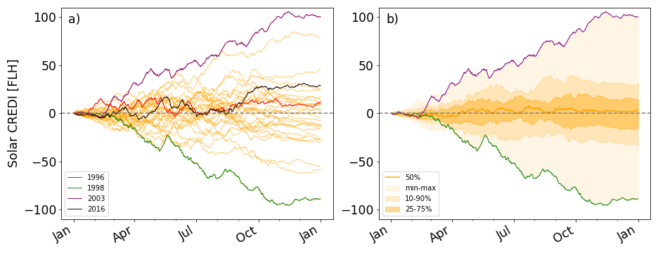
We define the credi to be the cumulative anomaly of a renewable resource with respect to its climate over a specific time period of interest from a chosen starting point in two steps (Figure 1). First, we determine the anomaly of a renewable resource, as the difference between the hourly generation potential of that resource and its climate (i.e. its expected value), taken from the computed hourly rolling window climate. Second, from an initial chosen starting point we sum these anomalies over a time period of interest.
More formally: let denote the generation potential for ordinal hour of year , and let denote the climate for ordinal hour for that potential . The anomaly of a renewable resource for ordinal hour of year is then defined as:
| (2) |
The credi over a given period of time is defined as the cumulative sum (or running total) of over that period. For example, if we align the starting point with the start of the year, the credi on the -th hour of that year () is:
| (3) |
When interpreting the index, the following should be considered. A change in credi over time is an indication of either an excess or deficit of the renewable resource potential with respect to its climatic normal (Figure 1b). A stable credi over a period indicates nominal renewable resource potential with respect to its climate.
Specifically, the credi score has the unit Full Load Hours (FLH) and at a given time informs the user of the cumulative surplus or deficit generation potential over the period considered with respect to its nominal behaviour. So given a fixed time window, the distribution of the credi score calculated then provides insight into the properties of a connected storage unit, like the (dis-)charge potential. FLHs depend on the installed capacity, therefore if the installed capacity of a resource is known or assumed, the index allows for direct assessment of the storage volume and power needed to always generate nominally within the fixed time window used.
For clarity, when the index is applied to a specific resource, we first refer to the resource before the index acronym is given. For example, the wind credi refers to an assessment of the credi of wind energy potential, and similarly for solar.
2.3 The use of storylines in analysing credi
The index can be used to assess the temporal development of anomalous renewable energy generation. In line with the application of hydrological drought indices, a physical storylines approach [31, 32] could be used. This approach can use regional climate change information while avoiding the strict limitations of a normal confidence-based approach applied in climate science. Storylines can be used to gain more insight into the driving processes, identify event analogues, and investigate similar events in alternative energy systems or under future climate conditions. Utilising these insights in, for example, resource adequacy assessments or system design studies, will likely lead to a more robust energy system.
Selection of relevant events can be based on historical adequacy assessments (like the [33] Adequacy Outlook). As shown by [12, 32], event analogues can then be found in large energy-climate datasets that incorporate climate change [1, 11]. By studying these analogues the physical processes and likelihood of these events can be assessed.
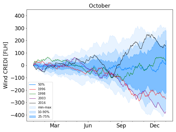
To demonstrate the index at different timescales and to highlight relevant considerations in the application of the credi, we selected the years 1996, 1998, 2003 and 2016 as storylines. The year 1996 was chosen specifically, as one of the most challenging years for resource adequacy in the Netherlands and Germany in a future net-zero emission energy system [[]p.56]tennet2023. In the analysis of the potential for hydrogen generation from wind, 2003 and 2010 where found to be anomalously low [[]p.58-61]tennet2023. Both 1998 and 2016 where chosen as they represent the most anomalous years of the index for solar and wind, respectively.
3 Data
We used the preliminary 4th version of the Pan-European Climate Database to demonstrate the credi in this paper [[, PECDv4.0;]]Dubus2022PECD. This database, developed by Copernicus Climate Change Services (C3S) in cooperation with the European Network of Transmission System Operators for Electricity (ENTSO-E) will be the new standard database used for all common Transmission System Operator (TSO) studies. The full database will be openly available as part of the new C3S-Energy dataset, expected in late 2023 (https://climate.copernicus.eu/energy/).
To showcase the developed index all figures show data from the preliminary PECDv4.0 of the northern region of the Netherlands. This region is the NUTS statistical region ‘NL1’ and covers the provinces of Groningen, Friesland and Drenthe, see: https://en.wikipedia.org/wiki/NUTS_statistical_regions_of_the_Netherlands. While the region is named ‘NL01’ in the PECD dataset, the NUTS-code is used here. While we focus in the main paper on the NL1 region, in the supplement we show additional regions reflecting some of the diversity within Europe. Further details in SI Section F.
4 Application of the credi at different timescales
In this section we show the application of the index at decadal, seasonal and sub-seasonal timescales in the context of modelling future energy systems. The considerations associated with choosing a starting point for the credi calculation is especially relevant at (sub-)seasonal timescales, and will be discussed.
On daily timescales the weather is extremely variable, but it depends on local conditions and short-term battery storage comes into play [34]. For most regions the maximum cost-effective storage based on the surplus charging capacity from wind and/or solar is in the order of 8 hours to 4 days [35, 36, 34]. For these reasons, we make no assessment on daily timescales here. However, due to the relevance of short-term events for the energy system, an example of a 8-day study window in credi is provided.
4.1 Annual to decadal variability in credi
At annual to decadal timescales the index can be used to assess the impact of large scale oscillations in the ocean and atmosphere on the availability of a renewable energy resource. These long-term deviations from the climate are relevant, e.g., because they offer sources of meteorological predictability [37, 38], or because stakeholders look at 10 year time periods to estimate return of investments [33].
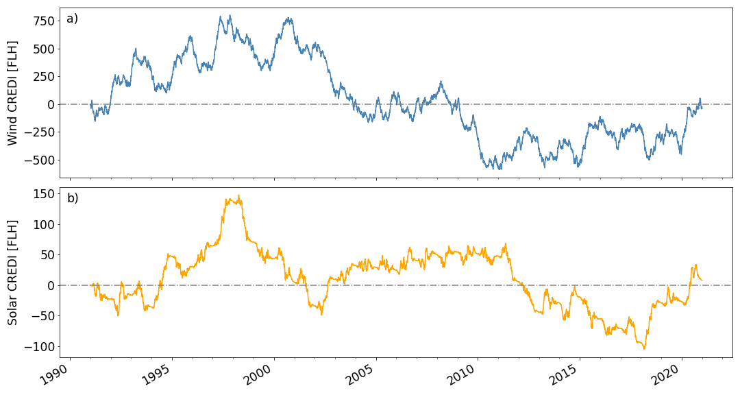
Over the past 30 years, large inter-annual variation is observed in the wind credi (Figure 3a). The cumulative effect of variations at seasonal scales resulted in higher than expected wind generation potential from 1991 to 2002, while from 2010 onwards wind credi declined indicating lower than expected wind generation potential. These general variations are in line with those found by [39, 15].
Similarly, the solar credi shows inter-annual variability. From 1991 to 2003 solar credi shows a general decrease, indicating less than average potential generation from solar. Within this period, a strong reduction in the periods 1993-1995 and 1998-2002 is observed (Figure 3b). In the period 2005-2018, solar credi is flat, showing that the solar potential was as expected from climate. After this period a steady increase in the solar credi is observed, indicating higher than expected potential generation.

The values of solar credi are generally lower than those of the wind credi. This is directly related to the diurnal cycle, which by definition gives zero solar potential at night and low values in the morning and evening. Consequently, the sum of the anomalies over a given period is smaller than for wind potential, which has values for all 24 hours in a day.
Finally, while the impact of the relative observed variability depends on the ratio of installed capacities, we observe that the inter-annual energy-meteorological variability is mainly driven by the wind resource in the analysed region (i.e., the northern of the Netherlands). And though the wind and solar credis show strong anti-correlated behaviour during some years (e.g. from 1991 to 2002), in others this is not the case (e.g. from 2004 to 2005). At decadal timescales, wind and solar balance the system somewhat, but they are not suited to fully negate the variability of their counterpart.
4.2 Seasonal variability in credi
When assessing the seasonal energy-meteorological variability using the credi, the starting point determines the way the temporal development of the index is perceived. In line with definitions of hydrological drought, the starting point determines the separation between energy surplus (wet) and deficit (dry) years. As the index is intended to capture the energy-meteorological variability, the start date is picked such that the biggest range if credi at the end of, and throughout, the year is observed.
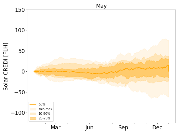
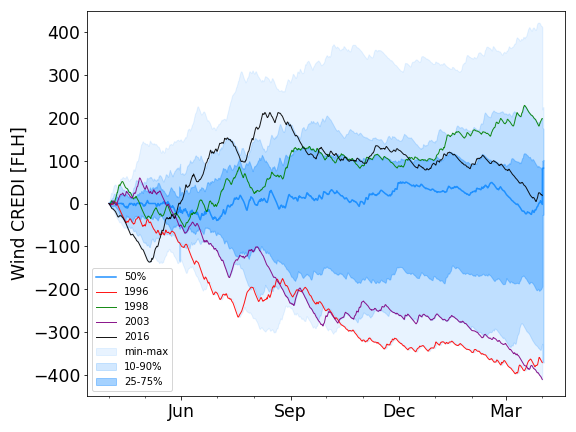
Comparing credi starting points for each month of the year, we found that these should not be the same for wind and solar (SI Section B). We use May 1st as the starting point for wind, as it gives the widest distribution of the index at the end of the analysis window in this particular region. For solar no clear distinction is found between a December or January starting point, we chose to use January 1st here.
For the yearly wind credi, it is obvious that an individual year can either be anomalously positive or negative, and that variations throughout a year are large (Figure 4a). This results in a wide range of yearly storylines. The 25-75% spread of the index grows to FLH over a year (Figure 4b). The most extreme negative year in the period considered for wind credi was 2016. In that year, from about September onwards, the wind potential was almost consistently below expected with less FLHs at the end of the analysed period.

As an example of the use of wind credi for storyline analysis we look at 1996. From May to October the index is relatively flat, indicating that the wind potential was as expected from its climate (red line in Figure 4b). Then, a strong reduction is observed in the wind credi from December to the end of January, indicating much lower then average potential generation from wind. Part of this deviation is compensated by higher than normal generation potential in February of 1997.
As noted earlier, values of yearly solar credi are smaller than of wind credi (Figure 5a), with an average spread (25-75%) of FLHs, and uncommon spread (10-90%) of FLHs spread over a year (Figure 5b). This indicates that ~18 FLHs of total energy is needed to cover the deficit of the installed solar capacity in 50 % of years and ~35 FLHs to cover 80% of years (Figure 5).
The most extreme year of high solar potential was 2003; the most extreme year of low solar potential was 1998. Especially 2003 is remembered for its extremely warm and sunny summer [40].
4.3 Sub-seasonal variability in credi
At sub-seasonal timescales, similar to seasonal, the start point determines the way the temporal development of the index is perceived. We use ’energy’-seasons to capture the large scale changes on sub-seasonal timescales. For wind we define two seasons of interest: September to March, and April to August. For brevity, only the results found for wind in the winter ‘energy’-season are shown here, see SI Section C for the other and solar. Alternative definitions of ’energy’-seasons can be relevant, especially for regions that have different sub-seasonal behaviour then the ‘NL1’-region shown here.
It is obvious that different years show quite different characteristics (Figure 6a) and individual winter seasons can differ greatly. As expected, the sub-seasonal timescale is emphasised more. For instance, the anomalous index-development in 1996 described in Section 4.2 is more clearly visible. Especially the strong reduction in wind credi from December to the end of January stands out as a period of much lower than normal wind generation potential.

4.4 A short-term study window for event-based credi
Finally, short-term events, e.g. Dunkelflautes, can pose significant risk to highly renewable energy systems [41, 42, 12, 43, 44]. A 8-day window for credi aligns with previous work [33], and is investigated here, see SI Section D for additional figures and the top 50 8-day events.
For short-term event analysis we do not pre-define the start point, all 8-day windows are considered. Overlapping events that share a five or more days, are removed from the analysis. While we only consider the lowest final credi value for our event selection, other impact selection methods as described by [32] can be used.
Again we noted the large weather-caused variability between different 8-day periods (Figure 7a). The computed spread in Figure 7b considers events throughout the year. This can also be investigated on a seasonal basis for winter or summer-specific event information, or for shorter or longer events.
The most extreme event is from 16-24 jan. 2017 and the analysis year 2016 is present 3 times in the top 50 events. While the specific 8-day event found in [33] is not the most extreme event, the analysis year 1996 does show up four times in the top 50 events. Indicating that the analysis year 1996 indeed stands out as quite exceptional.

5 Discussion
The presented index is defined as the cumulative anomaly of a renewable resource with respect to its climate. The method of determining the climate is thus vital and, as shown, should take into account the strong diurnal and annual cycle present in renewable energy resources. The calculation of the climate used here has a dependence on the size of the rolling window, which was primarily based on expert judgement. A longer timeseries, covering many decades, could be used for a cross-validation check to obtain the optimum rolling window size, but the data source should be selected with great care, due to potential inconsistencies [39, 45, 46]. In previous work a climatic definition on harmonics has been effective [47, 48, 49], but we found it unsuitable here (see SI Section A.3).
credi should not be confused with the standardised energy indices recently introduced by [18]. While we have been inspired by indices for monitoring hydrological droughts, their standardised energy indices are direct analogues. Meaning that those indices are a pure statistical assessment of the observed variance that rely heavily on the empirical distribution functions used [[, See Section 2]p.2-3]Allen2023. However, in energy system operation and control, the specific sequence of observations and the deviation with respect to the expected patterns matter. The credi presented incorporates these aspects.
When combined with weather forecasts, indices for hydrological drought can help policy makers make early decisions regarding societal risks [23, 24, 25, 26]. However, the operation of the electricity grid requires balance on very short timescales [1, 33]. While we presented our index with an hourly resolution, further research is needed to investigate if the credi can also be applied on these very short timescales. The examples provided, however, do already show credi’s usefulness in resilience planning, resource adequacy assessments, and as a metric for selecting events for robustness analysis.
In this introduction of the index, we applied it to the northern region of the Netherlands. However, as shown by [50], energy-meteorological variability is strongly region dependent. Therefore, the credi should be calculated and analysed for each region separately. Due to the ease of application, and the intuitive analysis and interpretation of the index, this application to other regions is relatively straightforward (see SI Section E for a few additional regions).
6 Conclusion
Drawing inspiration from the work on drought monitoring indices, we have presented the hourly rolling window climatology and Climatological Renewable Energy Deviation Index (credi). Given the relevance of both the diurnal and annual cycle in meteorology for energy applications, we recommend a simple but suitable definition of the background climate using an hourly rolling window approach. This new index is meant as an analytical method for researchers and stakeholders to help them understand and explain the impact of the variable nature of the weather on the energy system. The index computes the cumulative deviation or anomaly from the climatology for a chosen period.
The index can be used when understanding of energy-meteorological variability is key. For example, the credi can be used as part of a resource adequacy analysis from TSOs to identify events which are likely to be a challenge in maintaining security of supply in a (future) power system driven by renewable energy sources. At the same time, the credi could be used to assess the volume and power output of back-up resources needed for a given timescale, region, and energy system design. Then, by using the event selection and analysis, as e.g. in [32] for hydrological extremes, detailed event descriptions can be developed, systems can be stress tested, and further insight could be gained into energy-meteorological variability.
CRediT Author Statement
Conceptualisation, Formal Analysis and Visualisation: LPS, Investigation, Methodology and Writing - Original Draft: LPS, KvdW, Writing - Review & Editing: All listed authors, Supervision and Funding acquisition: AJF, MvdB.
Acknowledgments
Laurens P. Stoop received funding from the Dutch Research Council (NWO) under grant number 647.003.005. The content of this paper and the views expressed in it are solely the author’s responsibility, and do not necessarily reflect the views of TenneT TSO B.V..
Open research
The implementation of the credi, its use at different timescales, all code used to generate the figures, the data from the ‘NL1’ region discussed and the full list of the most extreme short-term events found as presented in this study are available at Github via https://github.com/laurensstoop/ccmetrics with the MIT license.
The full preliminary dataset of the PECDv4 containing the regional renewable resource potential for other technological definitions of wind and solar, or regions, then used in this study are not available due to ongoing validation. In due time the full PECDv4, including raw gridded and aggregated regional/national renewable resource potentials for a wide range of technological definitions, will be made available as part of the C3S Energy dataset and can be found through https://climate.copernicus.eu/operational-service-energy-sector. The framework describing the new C3S-Energy dataset, part of which is the PECDv4, can be found on: https://climate.copernicus.eu/c3s2412-enhanced-operational-services-energy-sector.
References
- [1] Michael T. Craig et al. “Overcoming the disconnect between energy system and climate modeling” In Joule, 2022 DOI: 10.1016/j.joule.2022.05.010
- [2] H.. Bloomfield et al. “The Importance of Weather and Climate to Energy Systems: A Workshop on Next Generation Challenges in Energy–Climate Modeling” In Bulletin of the American Meteorological Society, 2021 DOI: 10.1175/bams-d-20-0256.1
- [3] Russell McKenna et al. “High-resolution large-scale onshore wind energy assessments: A review of potential definitions, methodologies and future research needs” In Renewable Energy, 2022 DOI: 10.1016/j.renene.2021.10.027
- [4] David EHJ Gernaat et al. “Climate change impacts on renewable energy supply” In Nature Climate Change, 2021 DOI: 10.1038/s41558-020-00949-9
- [5] Rogier H. Wuijts, J.M. van den Akker and Machteld Broek “Effect of modelling choices in the unit commitment problem” In Energy Systems, 2023 DOI: 10.1007/s12667-023-00564-5
- [6] James Price and Marianne Zeyringer “highRES-Europe: The high spatial and temporal Resolution Electricity System model for Europe” In SoftwareX, 2022 DOI: 10.1016/j.softx.2022.101003
- [7] Rogier H. Wuijts et al. “Linking Unserved Energy to Weather Regimes” In Submitted to: Earth’s Future, 2023 DOI: 10.48550/arXiv.2303.15492
- [8] Aleksander Grochowicz, Koen van Greevenbroek, Fred Espen Benth and Marianne Zeyringer “Intersecting near-optimal spaces: European power systems with more resilience to weather variability” In Energy Economics, 2023 DOI: 10.1016/j.eneco.2022.106496
- [9] Inès Harang, Fabian Heymann and Laurens P. Stoop “Incorporating climate change effects into the European power system adequacy assessment using a post-processing method” In Sustainable Energy, Grids and Networks, 2020 DOI: 10.1016/j.segan.2020.100403
- [10] Jing Hu et al. “Implications of a Paris-proof scenario for future supply of weather-dependent variable renewable energy in Europe” In Advances in Applied Energy, 2023 DOI: 10.1016/j.adapen.2023.100134
- [11] Laurent Dubus et al. “Towards a future-proof climate database for European energy system studies” In Environmental Research Letters, 2022 DOI: 10.1088/1748-9326/aca1d3
- [12] K. Van der Wiel et al. “Meteorological conditions leading to extreme low variable renewable energy production and extreme high energy shortfall” In Renewable and Sustainable Energy Reviews, 2019 DOI: 10.1016/j.rser.2019.04.065
- [13] Nils Ohlendorf and Wolf-Peter Schill “Frequency and duration of low-wind-power events in Germany” In Environmental Research Letters, 2020 DOI: 10.1088/1748-9326/ab91e9
- [14] Noelia Otero Felipe et al. “A Copula-Based Assessment of Renewable Energy Droughts Across Europe” In SSRN Electronic Journal, 2021 DOI: 10.2139/ssrn.3980444
- [15] Laurens P. Stoop, Erik Duijm, Ad Feelders and Machteld van den Broek “Detection of Critical Events in Renewable Energy Production Time Series” In Advanced Analytics and Learning on Temporal Data, 2021 DOI: 10.1007/978-3-030-91445-5\_7
- [16] L. Van der Most et al. “Extreme events in the European renewable power system: Validation of a modeling framework to estimate renewable electricity production and demand from meteorological data” In Renewable and Sustainable Energy Reviews, 2022 DOI: 10.1016/j.rser.2022.112987
- [17] Andy Boston, Geoffrey D Bongers and Nathan Bongers “Characterisation and mitigation of renewable droughts in the Australian National Electricity Market” In Environmental Research Communications, 2022 DOI: 10.1088/2515-7620/ac5677
- [18] Sam Allen and Noelia Otero “Standardised indices to monitor energy droughts” In Renewable Energy, 2023 DOI: 10.1016/j.renene.2023.119206
- [19] Peter H Gleick et al. “Regional hydrologic impacts of global climatic changes” In Arid Lands: Today and Tomorrow, 1985
- [20] Peter H. Gleick “Methods for evaluating the regional hydrologic impacts of global climatic changes” In Journal of Hydrology, 1986 DOI: 10.1016/0022-1694(86)90199-x
- [21] Thomas B McKee, Nolan J Doesken and John Kleist “The relationship of drought frequency and duration to time scales” In Proceedings of the 8th Conference on Applied Climatology, 1993 Boston URL: https://climate.colostate.edu/pdfs/relationshipofdroughtfrequency.pdf
- [22] Sergio M. Vicente-Serrano, Santiago Begueria and Juan I. Lopez-Moreno “A Multiscalar Drought Index Sensitive to Global Warming: The Standardized Precipitation Evapotranspiration Index” In Journal of Climate, 2010 DOI: 10.1175/2009jcli2909.1
- [23] Steven M. Quiring “Monitoring Drought: An Evaluation of Meteorological Drought Indices” In Geography Compass, 2009 DOI: 10.1111/j.1749-8198.2008.00207.x
- [24] James H. Stagge, Irene Kohn, Lena M. Tallaksen and Kerstin Stahl “Modeling drought impact occurrence based on meteorological drought indices in Europe” In Journal of Hydrology, 2015 DOI: 10.1016/j.jhydrol.2015.09.039
- [25] Carmelo Cammalleri et al. “The effects of non-stationarity on SPI for operational drought monitoring in Europe” In International Journal of Climatology, 2021 DOI: 10.1002/joc.7424
- [26] K. Van der Wiel, T.J. Batelaan and N. Wanders “Large increases of multi-year droughts in north-western Europe in a warmer climate” In Climate Dynamics, 2022 DOI: 10.1007/s00382-022-06373-3
- [27] Anthony Arguez and Russell S. Vose “The Definition of the Standard WMO Climate Normal: The Key to Deriving Alternative Climate Normals” In Bulletin of the American Meteorological Society, 2011 DOI: 10.1175/2010bams2955.1
- [28] World Meteorological Organization “WMO guidelines on the calculation of climate normals”, 2017 URL: https://library.wmo.int/doc%5C_num.php?explnum%5C_id=4166
- [29] IPCC “Annex IV: Modes of Variability [Cassou, C., A. Cherchi, Y. Kosaka (eds.)]” In Climate Change 2021: The Physical Science Basis. Contribution of Working Group I to the Sixth Assessment Report of the Intergovernmental Panel on Climate Change, 2021 DOI: 10.1017/9781009157896.018
- [30] Heinz Wanner et al. “North Atlantic Oscillation – Concepts And Studies” In Surveys in Geophysics, 2001 DOI: 10.1023/a:1014217317898
- [31] Theodore G. Shepherd “Storyline approach to the construction of regional climate change information” In Proceedings of the Royal Society A: Mathematical, Physical and Engineering Sciences, 2019 DOI: 10.1098/rspa.2019.0013
- [32] K. Van der Wiel, G. Lenderink and H. De Vries “Physical storylines of future European drought events like 2018 based on ensemble climate modelling” In Weather and Climate Extremes, 2021 DOI: 10.1016/j.wace.2021.100350
- [33] TenneT “Adequacy Outlook”, 2023 URL: https://www.tennet.eu/nl/nieuws/leveringszekerheid-van-elektriciteit-een-volledig-duurzaam-elektriciteitssyteem
- [34] Maximilian Parzen, Davide Fioriti and Aristides Kiprakis “The Value of Competing Energy Storage in Decarbonized Power Systems”, 2023 arXiv:2305.09795 [physics.soc-ph]
- [35] Hannah G. Livingston and Julie K. Lundquist “How many offshore wind turbines does New England need?” In Meteorological Applications, 2020 DOI: 10.1002/met.1969
- [36] Nestor A. Sepulveda et al. “The design space for long-duration energy storage in decarbonized power systems” In Nature Energy, 2021 DOI: 10.1038/s41560-021-00796-8
- [37] Ed Hawkins and Rowan Sutton “The Potential to Narrow Uncertainty in Regional Climate Predictions” In Bulletin of the American Meteorological Society, 2009 DOI: 10.1175/2009bams2607.1
- [38] A.. Scaife et al. “Skillful long-range prediction of European and North American winters” In Geophysical Research Letters, 2014 DOI: 10.1002/2014gl059637
- [39] Jan Wohland, Nour Eddine Omrani, Noel Keenlyside and Dirk Witthaut “Significant multidecadal variability in German wind energy generation” In Wind Energy Science, 2019 DOI: 10.5194/wes-4-515-2019
- [40] R. Garcia-Herrera et al. “A Review of the European Summer Heat Wave of 2003” In Critical Reviews in Environmental Science and Technology, 2010 DOI: 10.1080/10643380802238137
- [41] Paulina Tedesco, Alex Lenkoski, Hannah C Bloomfield and Jana Sillmann “Gaussian copula modeling of extreme cold and weak-wind events over Europe conditioned on winter weather regimes” In Environmental Research Letters, 2023 DOI: 10.1088/1748-9326/acb6aa
- [42] Fabian Mockert, Christian M. Grams, Tom Brown and Fabian Neumann “Meteorological conditions during Dunkelflauten in Germany: Characteristics, the role of weather regimes and impacts on demand”, 2022 DOI: 10.48550/ARXIV.2212.04870
- [43] Bowen Li, Sukanta Basu and Simon J. Watson “Automated Identification of “Dunkelflaute” Events: A Convolutional Neural Network–Based Autoencoder Approach” In Artificial Intelligence for the Earth Systems, 2022 DOI: 10.1175/aies-d-22-0015.1
- [44] Srihari Sundar et al. “Meteorological Drivers of Resource Adequacy Failures in Current and High Renewable Western U.S. Power Systems”, 2022 DOI: 10.31223/x57d2g
- [45] Jan Wohland “Process-based climate change assessment for European winds using EURO-CORDEX and global models” In Environmental Research Letters, 2022 DOI: 10.1088/1748-9326/aca77f
- [46] Clara Deser and Adam S. Phillips “A range of outcomes: the combined effects of internal variability and anthropogenic forcing on regional climate trends over Europe” In Nonlinear Processes in Geophysics, 2023 DOI: 10.5194/npg-30-63-2023
- [47] A.. Sabziparvar et al. “Geographical factors affecting variability of precipitation regime in Iran” In Theoretical and Applied Climatology, 2014 DOI: 10.1007/s00704-014-1174-3
- [48] M. Fischer, H.W. Rust and U. Ulbrich “A spatial and seasonal climatology of extreme precipitation return-levels: A case study” In Spatial Statistics, 2019 DOI: 10.1016/j.spasta.2017.11.007
- [49] Matthew D. Rayson, Nicole L. Jones, Gregory N. Ivey and Yankun Gong “A Seasonal Harmonic Model for Internal Tide Amplitude Prediction” In Journal of Geophysical Research: Oceans, 2021 DOI: 10.1029/2021jc017570
- [50] Bryn Pickering, Christian M Grams and Stefan Pfenninger “Sub-national variability of wind power generation in complex terrain and its correlation with large-scale meteorology” In Environmental Research Letters, 2020 DOI: 10.1088/1748-9326/ab70bd
- [51] P.. Bett, H.. Thornton and R.. Clark “European wind variability over 140 yr” In Advances in Science and Research, 2013 DOI: 10.5194/asr-10-51-2013
- [52] Yves-Marie Saint-Drenan et al. “An approach for the estimation of the aggregated photovoltaic power generated in several European countries from meteorological data” In Advances in Science and Research, 2018 DOI: 10.5194/asr-15-51-2018
- [53] Hans Hersbach et al. “The ERA5 global reanalysis” In Quarterly Journal of the Royal Meteorological Society, 2020 DOI: 10.1002/qj.3803
- [54] Juan Pablo Murcia et al. “Validation of European-scale simulated wind speed and wind generation time series” In Applied Energy, 2022 DOI: 10.1016/j.apenergy.2021.117794
- [55] Mads M. Pedersen et al. “PyWake 2.5.0: An open-source wind farm simulation tool”, 2023 URL: https://gitlab.windenergy.dtu.dk/TOPFARM/PyWake
- [56] Juan Pablo Murcia Leon, Matti Juhani Koivisto, Poul Sørensen and Philippe Magnant “Power fluctuations in high-installation- density offshore wind fleets” In Wind Energy Science, 2021 DOI: 10.5194/wes-6-461-2021
- [57] Graziela Luzia, Koivisto Matti and Andrea N. Hahmann “Validating Euro-Cordex Climate Simulations For Modelling European Wind Power Generation”, 2023 DOI: 10.2139/ssrn.4401025
Appendix A Comparison of Climatic Definitions of the Renewable Resources
Section 2 in the main text describes the four relevant timescales of energy-meteorological variability and shows the use of the hourly rolling window climate for renewable resources. Here we provide some additional detail on the observed variability of wind and solar potential (Section A.1) and an analysis on the specific behaviour during each hour of the day (Section A.2). We also highlight the use of different climate definitions (Section A.3) and discuss the sensitivity of the hourly rolling window climate on its window size (Section A.4).
A.1 Observed variability of wind and solar energy potential
Examples of typical behaviour of wind and solar energy are shown in Figure S1. For wind, at seasonal timescales, we observe lower mean generation potential in the summer period (Figure S1a, 2a. when weather conditions are more stable. The higher and more variable generation potential in the autumn and winter period is associated with the quicker succession of storms in Europe (Figure S1a,b).
For solar the difference between summer and winter is more pronounced, which is predominantly due to seasonal changes in the angle of declination of the sun (Figure S1d and 2c For both wind and solar the succession of large-scale high and low pressure systems can be observed (Figures S1b,e). Additionally, as the efficiency of solar panels declines with increasing air temperature, a reduced solar generation potential is observed around noon after the summer solstice (Figure S2).
On daily timescales the inherent diurnal cycle of the solar energy generation potential is very prominent and changes due to cloudiness are noticeable (Figure S1f). For the wind generation potential no diurnal cycle is evident (Figure S3), but large intra- to multi-day changes associated with the passing of weather systems can clearly be observed (Figure S1b,c).

The observed variability of wind and solar energy potential is in line with the large ensemble used by [12] and the decadal observations align with [51] and [39].
It is clear that both wind and solar show strong variability at daily to yearly timescales (Figure S1). To define a practically useful climate of the prevalent behaviour for the wind or solar energy resources, all these timescales of variability should be taken into account.
A.2 Climatic characterisation for each hour of the day
Section 2.1 in the main text describes the observed variability of wind and solar energy potential. Here we provide some additional figures (Figure S2 and S3) show the climatic behaviour throughout the year, for each hour of the day separately.
For solar, the strong annual and diurnal cycle are very clearly visible. In addition, a few peculiarities can be observed related to how solar panels function. The efficiency of solar panels declines with increasing air temperature [52], leading to a reduced solar generation potential around noon after the summer solstice from the higher temperatures at this time of the year.

For wind energy generation potential only the annual cycle of the seasonal variability of wind is clear and no clear distinction for the hour of the day can be made. The climatology for each hour of the day does not match perfectly and there are some minor differences observed.

A.3 Comparison of climate definitions
Section 2.2 in the main text discusses the climate of a renewable resource. Here we provide some additional figures showing that both a daily [28] and harmonic description of the climate are unsuitable for use in energy-meteorological applications (Figures S4 & S5). For the latter see the work of [47, 48, 49] for their use of the harmonic climate definition.
While the climate definitions are unsuitable, their impact on the crediis limited (Figure S6).


A.4 Sensitivity of window size for Hourly Rolling Window climate definitions
A comparison of windows for the hourly rolling window climate is shown in Figure S7 & S8 for solar and Figure S9 & S10 for wind.

For solar potential the hourly rolling window climate for a 10 day window is not suited as variations are observed on daily to weekly timescales that have no physical reason to be a recurrent over the years (see Figure S7). Similar to the climate for wind, these fluctuations observed at the 10 day window would not constitute as a good definition of a climate. On the other hand, very large windows like those using the 60, 90 or 120 window, are very smooth throughout the year, underestimating for instance the peak of maximum solar potential near the end of April/start of May (see Figure S8) and severely over estimating the winter dip in solar potential (Figure S7). Again, inline with what was found with wind this indicates an over-smoothing of the yearly cycle and thus using these windows within the hourly rolling window climate would thus not be a good indicator of likely weather. A window size in the range of 20-60 days is adequate in capturing the persistent weather fluctuations and the annual peak solar potential, without underestimating the annual cycle.

For wind potential the hourly rolling window climate for a 10 day window is not suited as variations are observed on daily to monthly timescales that have no physical reason to be a recurrent over the years (see Figure S10). As a climate is defined as the statistically-mean weather conditions prevailing in a region, the short-term nature of the fluctuations observed at the 10 day window would not constitute as a good definition of a climate as the climate fluctuates on short timescales. The same holds for the 20 day window, albeit to a lesser extent. On the other hand, very large windows like those using the 90 or 120 window, are very smooth throughout the year. For most of the mid-winter period their climate is well below the initial, simple average-based, climate and during the summer above (see Figure S9). This indicates an over-smoothing of the yearly cycle and thus using these windows within the hourly rolling window climate would thus not be a good indicator of likely weather. A window size in the range of 20-90 days is adequate in capturing the persistent weather fluctuations throughout the year, without underestimating the annual cycle.


Appendix B Annual start date analysis for credi
Section 4 in the main text describes the application of the credi at different timescales. Here we show how the hourly distribution of credi changes over a year if a different starting point is used (Figures S11 & S12). In line with the main text four exemplary storylines are shown, namely 1996 (red), 1998 (green), 2003 (purple) and 2016 (black).
From Figure S12, the impact of choosing a different starting point becomes very clear. For the storylines shown you can see that they change from one of the highest, to on of the lowest depending on the start point. To a lesser degree, the same holds for the solar resource shown in Figure S11.


Appendix C Additional seasonal analysis figures of credi
Section 4.3 in the main text shows the seasonal variability in credi. Here we provide some additional figures representing a different season for either wind or solar credi (Figures S13-S16).


Appendix D Additional short-term analysis figures of credi
Section 4.4 in the main text shows an example of the short-term credi event selection. Here we provide some additional figures related to the event selection and the observed behaviour. Figure S17 shows the wind distribution of the generation potential during the analysis period and for the selected events.

The distribution of all non-overlapping events in the analysed period for both solar credi and wind crediis shown in Figure S18. This is then further detailed by looking at the wind credi and solar credi values at the end of the selected events for both wind and solar in Figures S19 and S20, where the latter only shows the top 50 events for both wind and solar. A Table with all top 50 events for both wind and solar credi 8-day events is provided in Table LABEL:tab:Top50longtable, see the Open Research section for the details of the code repository that contains the full list of all events.


| Event Rank | solar credi | Event date | wind credi | Event date |
|---|---|---|---|---|
| 1 | -15,49 | 23/05/2013 | -67,36 | 24/01/2017 |
| 2 | -13,98 | 18/05/1996 | -65,88 | 27/12/2006 |
| 3 | -13,80 | 07/06/2012 | -65,75 | 30/12/1992 |
| 4 | -12,97 | 06/05/2002 | -62,68 | 18/01/2013 |
| 5 | -12,55 | 08/07/2002 | -62,30 | 30/01/1991 |
| 6 | -11,82 | 26/05/2016 | -60,45 | 15/02/1993 |
| 7 | -11,75 | 11/07/2020 | -59,27 | 01/02/1992 |
| 8 | -11,30 | 18/06/1995 | -58,73 | 06/02/2006 |
| 9 | -11,16 | 23/05/1994 | -57,74 | 13/12/1996 |
| 10 | -10,93 | 28/05/2006 | -55,27 | 21/01/2001 |
| 11 | -10,89 | 14/05/2010 | -54,99 | 15/12/2001 |
| 12 | -10,88 | 28/07/2005 | -53,80 | 31/01/1997 |
| 13 | -10,82 | 31/07/1993 | -53,39 | 18/02/2008 |
| 14 | -10,44 | 21/03/1997 | -52,57 | 22/12/2007 |
| 15 | -10,44 | 31/07/2011 | -52,30 | 28/01/2004 |
| 16 | -10,43 | 13/06/1998 | -52,03 | 26/02/1994 |
| 17 | -10,30 | 17/03/2019 | -50,96 | 26/01/1997 |
| 18 | -10,12 | 12/05/2012 | -50,88 | 04/01/1993 |
| 19 | -10,07 | 09/04/1993 | -50,61 | 02/03/2019 |
| 20 | -10,00 | 12/05/2014 | -50,54 | 26/01/2019 |
| 21 | -9,92 | 13/08/1993 | -50,41 | 03/02/2001 |
| 22 | -9,88 | 14/06/2010 | -50,34 | 13/01/1997 |
| 23 | -9,84 | 22/07/1993 | -50,13 | 13/01/2002 |
| 24 | -9,74 | 26/03/2016 | -50,08 | 07/03/2021 |
| 25 | -9,67 | 09/05/2010 | -49,91 | 17/02/1991 |
| 26 | -9,65 | 05/04/2000 | -49,82 | 24/11/2011 |
| 27 | -9,63 | 20/07/2011 | -49,03 | 21/12/2016 |
| 28 | -9,39 | 13/07/2000 | -48,58 | 11/01/2003 |
| 29 | -9,34 | 01/07/1996 | -48,47 | 14/12/2004 |
| 30 | -9,17 | 03/07/1991 | -48,29 | 24/12/2021 |
| 31 | -9,14 | 21/04/1992 | -48,21 | 22/11/1998 |
| 32 | -9,01 | 06/05/2005 | -48,19 | 23/12/2017 |
| 33 | -9,00 | 20/06/1993 | -48,14 | 16/10/1994 |
| 34 | -8,99 | 10/09/1995 | -47,60 | 03/11/1997 |
| 35 | -8,97 | 03/05/2019 | -47,44 | 05/12/2004 |
| 36 | -8,97 | 31/05/1998 | -47,20 | 04/12/1991 |
| 37 | -8,97 | 17/07/1998 | -46,51 | 07/02/2015 |
| 38 | -8,95 | 31/03/2015 | -46,47 | 26/01/2015 |
| 39 | -8,95 | 31/05/2014 | -46,44 | 04/02/1991 |
| 40 | -8,93 | 02/06/2007 | -46,38 | 09/12/1991 |
| 41 | -8,92 | 17/06/1991 | -46,31 | 09/01/2010 |
| 42 | -8,89 | 08/03/2012 | -46,30 | 23/02/2013 |
| 43 | -8,88 | 25/05/2003 | -46,24 | 29/01/2017 |
| 44 | -8,86 | 14/08/2001 | -45,76 | 13/01/2013 |
| 45 | -8,85 | 20/04/2005 | -45,51 | 18/02/2003 |
| 46 | -8,84 | 01/07/2017 | -45,25 | 16/01/2001 |
| 47 | -8,82 | 30/09/1991 | -45,16 | 17/03/1991 |
| 48 | -8,82 | 09/10/1998 | -44,90 | 24/02/2018 |
| 49 | -8,81 | 26/07/2011 | -44,87 | 27/01/2010 |
| 50 | -8,80 | 08/05/1991 | -44,46 | 17/10/1995 |
Appendix E Application of credi to other regions
Section 5 in the main text discusses the use of the credi for other regions. Here selected additional figures on the application of the index and very limited analysis for some other regions is provided. Due to the preliminary version of the PECDv4.0 used, caution is advised on the exact interpretation of the results and no data is provided for these regions. In addition, for the analysis only the seasonal and annual to decadal variability is discussed as the analysis of the short-term and sub-seasonal variability depends on the choice of the storylines which depend on the region considered and are kept consistent with the main text for reference.
The additional regions used are Slovakia (‘SK00’), the southern tip of Sweden (‘SE02’) and one of the south-east regions of France (‘FR10’). The choice for these regions was made to reflect some of the diversity within Europe. Not all regions are shown for all figures provided in the main text, the figures not shown can be found as listed in the Open Research section on github.
E.1 Observed variability of wind and solar energy potential — Other regions
Similar observations can be made on the timescales of variability for the other regions then the ‘NL1’ region discussed in the main text (Figure S21). While the distribution of the values differs between regions, similar characteristics are observed. For wind at seasonal timescales a lower mean generation potential is observed in all three regions (‘SK00’ not shown). Some shifts in the characteristic behaviour can be observed. For instance, there is lower solar generation in winter for more northern regions, and a more strongly pronounced skewness of the solar generation potential throughout the year is seen for ‘SE02’.


E.2 A hourly rolling windows climate — Other regions
The hourly rolling window climate defined in Section 2.2 of the main text was applied without any changes to the other regions considered. As can be seen in Figure S22, this climate provides a smoother description of the expected behaviour on annual timescales and reduces the random fluctuations.
In line with the observations for the northern region of the Netherlands, the initial, simple average-based climate does capture the annual timescales, but shows random fluctuations from day-to-day and hour-to-hour. For both Slovakia and the part of Sweden shown some consistent daily variation is observed for their wind generation potential, whether this is from a physical driver is unknown and should be further studied before using the climatic description for these regions.


E.3 Annual to decadal variability — Other regions
Section 4.1 in the main text discusses annual to decadal variability observed in the credi, here we shortly discuss the same for other regions.
Over the past 30 years, large and consistent inter-annual variation is observed in the wind credi for the ‘FR10’ region (Figure S23), while the ‘SE02’ region shows more variable behaviour on annual and seasonal timescales (Figure S24). For the French region, some cumulative effect over the whole period can be observed, while the Swedish region shows a more oscillating pattern.
Similar to the ‘NL1’ region, more inter-annual periods with a flat solar credi can be observed then for wind. For the French region a general decrease of the solar credi, thus anomalous low generation potential, is observed in the period 1992-2004 and a very consistent increase from 2018 to 2021. For the Swedish region a yearly flat solar credi is observed, likely related to the very limited solar generation potential in the winter.

E.4 Seasonal variability — Other regions
Section 4.2 in the main text discusses seasonal variability in the credi, here we shortly discuss the same for the ‘SE02’ region as it shows the most interesting properties (see Figure S25).
The wind credi in this Swedish region shows similar behaviour as the Dutch region discussed in the main text, but while the 2016 storyline is considered to be the most extreme for the northern region of the Netherlands, this is not the case for the ‘SE02’ region. In addition, the shape of the distribution of the wind credi is different throughout the year and the 1996 storyline shows the highest wind credi value. This stark opposition to the behaviour observed in that storyline for the Netherlands indicates some possible balancing for this specific storyline.
The solar credi in the southern Swedish region ‘SE02’ shows a very flat value in the period from October to March. This is likely due to the very clearly limited solar generation potential in this region during the wintertime period and the reasons for the limited annual to decadal variability observed for this region (see Figure S24). At the same time large seasonal differences between the different March to September periods are observed. As for the ‘NL1’ region, the year 1998 is the most extreme storyline for solar credi.


Appendix F Extended Data section
We used the preliminary 4th version of the Pan-European Climate Database to demonstrate the credi in this paper [[, PECDv4.0;]]Dubus2022PECD. This database, developed by Copernicus Climate Change Services (C3S) in cooperation with the European Network of Transmission System Operators for Electricity (ENTSO-E) will be the new standard database used for all common Transmission System Operator (TSO) studies. The full database will be openly available as part of the new C3S-Energy dataset, expected in late 2023 (https://climate.copernicus.eu/energy/). To showcase the developed index all figures show data from the preliminary PECDv4.0 of the northern region of the Netherlands (‘NL1’).
Within PECDv4.0 a range of technological properties have been modelled for both wind turbines and photovoltaic solar panels [11]. Only the historic hourly generation potential (or capacity factor) timeseries are used for solar and wind with the properties of ‘existing technologies’. Our subset uses the ERA5 reanalysis for its meteorological forcing [53]. The wind power plant conversion model is the generic power curve model presented in [54] that is implemented in PyWake [55]. For the property parameterisation it uses the 2020 data from the WindPowerNet (https://www.thewindpower.net/). Storm shut down behaviour is modelled after [56], while wakes are modelled as part of the generic power curve and for other losses a 10% reduction factor is applied [57]. The regional solar photo-voltaic (PV) potential is derived following [52]. A distribution of near optimal tilt and azimuth angles was used that reflects current installed capacities. For aggregation to the modelled zones in the PECDv4.0 database, the gridded ERA5 data was weighted by the cover of protected areas, regions with high slopes and/or high elevation.