The Cheeger constants of random Belyi surfaces
Abstract.
Brooks and Makover developed a combinatorial model of random hyperbolic surfaces by gluing certain hyperbolic ideal triangles. In this paper we show that for any , as the number of ideal triangles goes to infinity, a generic hyperbolic surface in Brooks-Makover’s model has Cheeger constant less than .
1. Introduction
Given a closed hyperbolic surface of genus , the Cheeger constant of is defined as
where runs over all one-dimensional subsets of dividing into two disjoint components and , and is the length of . The Cheeger constant can bound the first eigenvalue of from both sides. Actually the well-known Cheeger-Buser [9, 8] inequality says that
In particular, if and only if . For large genus, by Cheng [10] it is known that
| (1) |
for any sequence of hyperbolic surfaces of genus .
Brooks and Makover [4] developed a combinatorial model of a random closed surface with large genus by first gluing together copies of an ideal hyperbolic triangle and then taking its conformal compactification, where the gluing scheme is given by a random trivalent graph. It is known (e.g., see [11, Lemma 2.1]) that such constructions give all the so-called Belyi surfaces which are dense in the space of all Riemann surfaces in some sense (e.g., see [1]). In this model, certain classical geometric quantities were studied for large . For example: as the parameter , they showed [4, Theorem 2.3] that the expected value of the genus of a random hyperbolic surface roughly behaves like ; they also showed [4, Theorem 2.2] that as , a generic hyperbolic surface in their model has Cheeger constant greater than where is an implicit uniform constant. For the other direction, in light of (1) it is natural to ask
Question.
Is there an so that as , a generic hyperbolic surface in Brooks-Makover’s model has Cheeger constant less than ? If yes, similar as in [5], can be chosen to be greater than ?
Now we briefly recall the terminologies in Brooks-Makover’s model of random hyperbolic surfaces [4]. Set
As in [4], each pair gives two Riemann surfaces and where is an open Riemann surface constructed by gluing ideal hyperbolic triangles in a certain way, and is the conformal compactification of . Let be the uniform measure on introduced by Bollobás [2], which one may also see [4, Section 5] for more details. In this paper we prove the following result which in particular gives a positive answer to the question above. More precisely,
Theorem 1.
Let be a random element of . Then for any ,
Remark.
- (1)
-
(2)
For the non-compact case, recently we showed in [24] that as the genus goes to infinity, a Weil-Petersson cusped hyperbolic surface has arbitrarily small Cheeger constant provided that the number of cusps grows significantly faster than .
-
(3)
By Buser’s inequality [8], a uniform spectral gap also yields a uniform positive lower bound for Cheeger constant. For this line, one may see e.g. [23, 12, 15, 18, 16] for congruence covers of the moduli surface ; see e.g. [19, 20, 14] for random covering surfaces; and see e.g. [21, 26, 17, 13] for Weil-Petersson random surfaces.
We remark here that after this paper was submitted, very recently Budzinski, Curien and Petri showed in [7] that
for any sequence of hyperbolic surfaces of genus . This solved [25, Problem ] due to Wright. It would be interesting to know that whether this upper bound can be replaced by .
Strategy on the proof of Theorem 1.
We briefly introduce the idea on the proof of Theorem 1 here. By definition of the Cheeger constant, it suffices to show that for a generic surface , there exists a colletion of curves whose union separates into two parts such that the ratio quantity in can be bounded from above by the desired upper bound in Theorem 1. By the construction of hyperbolic surfaces in [4], we know that
where each is a horoball in together with its infinity point, and each small triangle has three boundary curves of lengths (for example see Figure 8). For large and a generic surface , we first split as where each with contains a hyperbolic disk of large radius (see Section 3). Next we construct certain simple curves of lengths at most separating each into certain subdomains , each of which has area at most (see Lemma 6). Rewrite the decomposition as
Then one can make divisions of as follows: fix two symbols and define the so-called compatible mapping such that
-
(1)
on the interior of each piece of the decomposition of above, is constant either or ;
-
(2)
for three horocycle segments in any small triangle, there exists at most one of them such that it (if exists) is contained in the boundary where
Each map induces a division of (for example see Figure 8). Define to be the set of all compatible mappings from to , which is a finite set endowed with a uniform probability measure. Now we view and as two random variables on . Here the randomness only comes from the mapping and the surface is fixed. With the help of Lemma 6 we show that for almost a generic defined in (8), the expected values satisfy
Plan of the paper.
Section 2 provides some necessary background from [4] and basic properties on two-dimensional hyperbolic geometry. In Section 3, based on [3, 4] we provide several bounds on hyperbolic lengths and areas, and also give a special division for certain disks from a decomposition of which is important in the proof of Theorem 1 (see Lemma 6). We prove our main result Theorem 1 in Section 4.
Acknowledgements.
The authors would like to thank the anonymous referees for their careful reading and valuable comments, and especially would like to thank one referee for sharing his/her idea on how to obtain the current upper bound in Theorem 1, improving our former one . They significantly improve the quality of this paper. We also would like to thank Yuhao Xue for helpful discussions, and thank Bram Petri and Zeev Rudnick for their interests and comments on this project. The second named author is partially supported by the NSFC grant No. .
2. Preliminary
The Belyi surfaces are compact Riemann surfaces which can be defined over the algebra number field . From [1, Theorem 1] we know that a compact Riemann surface is a Belyi surface if and only if there exists a covering unramified outside . In this section, we will mainly review the construction of Belyi surfaces as in [4] by Brooks and Makover. For related notations and properties, the readers may also refer to [4, section 4] for more details.
2.1. Two dimensional hyperbolic geometry
Let be the upper half-plane endowed with the standard hyperbolic metric
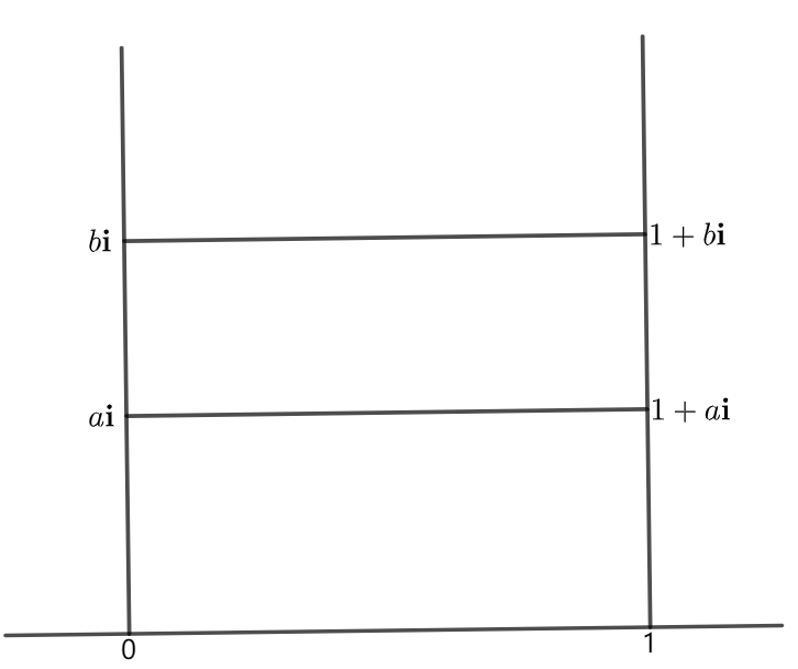
For any , set
Then their hyperbolic lengths satisfy
| (2) |
We also set
Then its hyperbolic area satisfies
| (3) |
2.2. Construction of Belyi surfaces
Now we recall the construction of Belyi surfaces in [4], i.e., the surface associated with an oriented graph . Let be a finite regular graph and be the set of all its vertices. An orientation on is an assignment, for each vertex , of a cyclic ordering for the three edges emanating from . Set
| (4) |
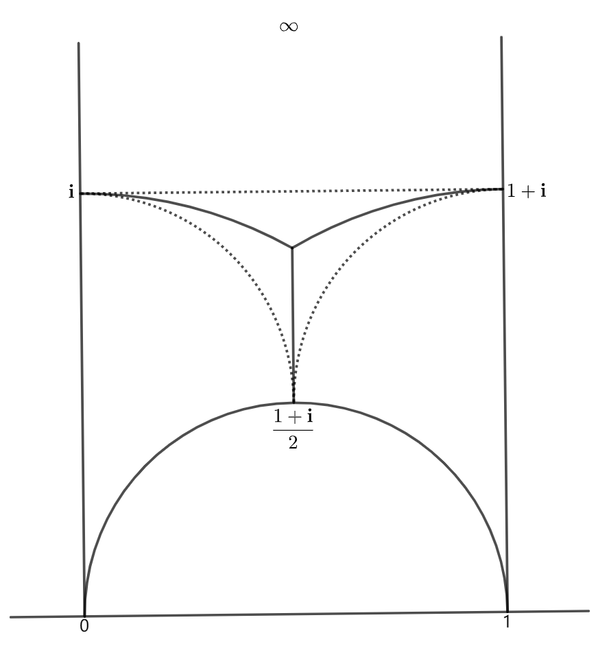
Up to a Möbius transformation, one may assume that an ideal triangle always has vertices and (see Figure 2). The solid segments are geodesics joining the point and the points in . The dotted segments are horocycles joining pairs of points in . The ideal triangle has a natural clockwise orientation
In this article, similar as in [4], the points are called the mid-points of the three sides of , even each side has infinite length. And a dotted segment (see Figure 2) joining two mid-points of an ideal triangle is always called a short horocycle segment. It is clear that each short horocycle segment has hyperbolic length equal to .
Given an element , we replace each vertex by a copy of , such that the natural clockwise orientation of coincides with the orientation of at the vertex . If two vertices of are joined by an edge, we glue the two copies of along the corresponding sides subject to the following conditions:
-
(i)
the mid-points of two sides are glued together;
-
(ii)
the gluing preserves the orientations of two copies of .
As in [4], the surface is uniquely determined by the two conditions above, and it is a complete hyperbolic surface with area equal to .
Definition.
The compact Riemann surface is defined as the conformal compactification of by filling in all the punctures.
It is known that a Riemann surface is a Belyi surface if and only if can be represented as
for some (e.g., see [11, Lemma 2.1]).
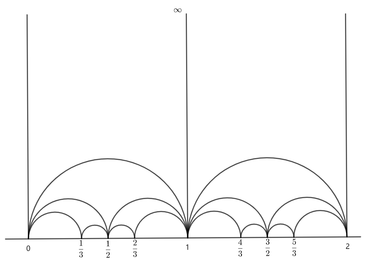
For any points , denote by the hyperbolic geodesic line joining and , and denote by the ideal triangle with vertices and . Let and be the matrices as follows:
They represent the following two automorphisms of :
Then and generate a subgroup of . Set
Then the set consists of ideal triangles forming a partition of the upper half-plane as in Figure 3.
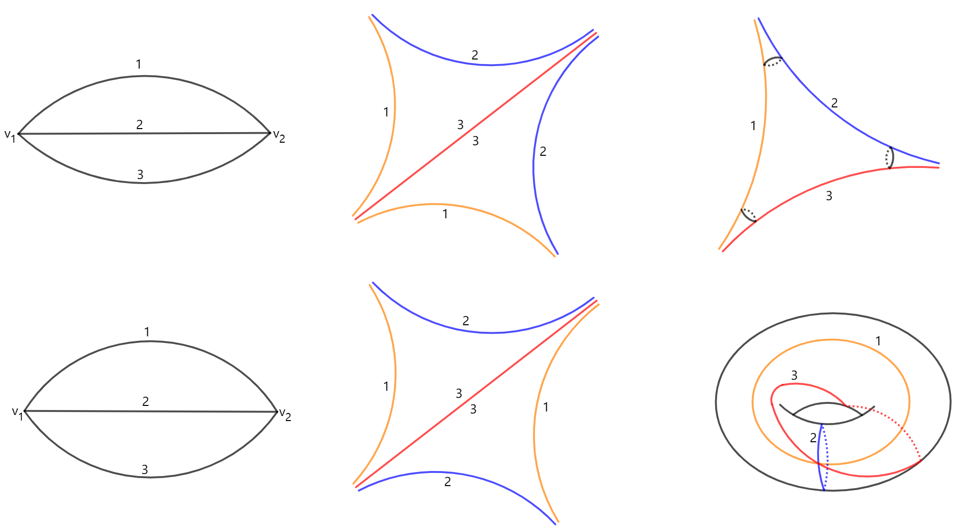
There exists a fundamental domain of in such that it is a finite union of ideal triangles in . For example, let and be two vertices of a regular graph as shown in Figure 4, and the orientations at and are and respectively. From the construction of , it is not hard to see that the union
is a fundamental domain of where the boundary sides and are identified, and the boundary sides and are identified. Then is a three punctured sphere (see Figure 4). Using the same regular graph , consider the orientation such that the orientations at the two vertices are both as shown in Figure 4, then is a torus with one puncture.
2.3. Horocycles around punctures
Recall that [4, Definition 4.1] says that a left-hand-turn path on is a closed path on such that at each vertex, the path turns left in the orientation . Every left-hand-turn path of corresponds to a horocycle loop in which encloses a puncture point and consists of certain short horocycle segments as described in subsection 2.2. One may denote such loops by canonical horocycle loops. For any two canonical horocycle loops, they are either disjoint or tangent to each other. We remark here that a canonical horocycle loop may also be tangent to itself. In the remaining, a tangency point always means either a tangency point between two canonical horocycle loops or a self-tangency point of one canonical horocycle loop.
Remark.
Since each ideal triangle contains three short horocycle segments and consists of ideal triangles, it follows that there are short horocycle segments for each hyperbolic surface .
For a random element , denote by the number of left-hand-turn paths in and by the expected value of over . Then is also the number of punctures of , and the genus of is equal to . We enclose this section by the following estimate which is a direct consequence of [4, Theorem 2.3].
Proposition 2.
There exist two universal constants independent of such that
Gamburd showed in [11, Corollary 5.1] that as . In this paper Proposition 2 of Brooks-Makover is enough for us where we only need the growth rate . For other geometric quantities of random surfaces in this model, one may also see Petri [22] for the behavior of the systole function; and see Budzinski-Curien-Petri [6] for the behavior of the diameter.
3. Bounds on lengths and areas
We start this section with the following assumption.
Assumption.
Throughout this paper, we always assume . So one may let and be the unique hyperbolic metrics on and associated to their complex structures respectively.
For any curve , we set
For any subdomain , we also set
Under such notations, by Gauss-Bonnet we have
| (5) |
3.1. Schwarz’s Lemma
The following estimate is well-known to experts. We prove it for completeness here.
Lemma 3.
Assume is a smooth curve and is a subdomain, then we have
In particular, for any short horocycle segment , we have
Proof.
Let be the natural holomorphic embedding
It suffices to prove that for any point and any tangent vector ,
Consider the following commutative diagram
where and are covering maps. Since is simply connected, there exists a holomorphic lift of , i.e.,
| (6) |
Since is holomorphic, it follows by the standard Schwarz’s Lemma that is -Lipschitz. Then the conclusion follows because both the covering maps and are local isometries. ∎
3.2. Large cusps condition
Given that is defined in (4), we let denote the set of all canonical horocycle loops of . Write the index set as for simplicity. For each , the canonical horocycle loop bounds a punctured disk with a puncture . Moreover is an open topological disk in .
Now we recall the so-called large cusps condition defined in [3, 4]. First for simplicity, we write and as and respectively. For any , up to a conjugation one may lift the puncture to in the boundary of the upper half plane . Let be the covering map with and assume that the Mobius transformation through doing one turn around corresponds to the parabolic isometry . For any , denote
and
Then for suitable , the set is a cusp around whose boundary curve is the projection of a horocycle. We also denote by the standard cusp
endowed with the hyperbolic metric. Now we recall [3, Definition 2.1] or [4, Definition 3.1] saying that.
Definition.
Given any , a hyperbolic surface has cusps of length if
-
(1)
is isometric to for any ;
-
(2)
for any .
Brooks and Makover in [4] proved that for any , as a generic hyperbolic surface has cusps of length . More precisely
Theorem 4.
[4, Theorem 2.1] Let be a random element of . Then for any ,
Let be the conformal compactification of endowed with the hyperbolic metric , i.e., . For any point and , denote
According to the proof of [3, Theorem 2.1], the following theorem holds.
Theorem 5.
[3, Theorem 2.1] For every , there exist two positive constants and which only depend on such that if has cusps of length , then we have
-
(1)
Outside of and we have
-
(2)
For any ,
Remark.
Now we take in Theorem 5 and fix the constant . From the remark above, we take such that
| (7) |
which will be applied in the subsequent subsection. Consider the following subset of which has large proportion to the whole set. More precisely, for any , we define
| (8) |
By Proposition 2 and Markov’s inequality we have
which together with Theorem 4 implies that for large enough,
| (9) |
Since the genus of is equal to , we have that for any ,
| (10) |
3.3. Divisions of disks
Let that is defined in (8). For each , we assume that the canonical horocycle loop around consists of short horocycle segments. So we have
| (11) |
where is the punctured disk enclosed by the canonical horocycle loop around in . Recall that each consists of ideal triangles each of which contains three short horocycle segments. So we have
| (12) |
Divide into the following two subsets
| (13) |
If , then for large enough we have
| (14) |
Recall that for every , is a topological disk in . For any , as in Figure 5, there are four closed loops around the puncture point as follows:
-
(a)
is the canonical horocycle loop under the hyperbolic metric ;
-
(b)
is the horocycle loop with length under the hyperbolic metric ;
-
(c)
is the horocycle loop with length under the hyperbolic metric ;
-
(d)
the loop is the boundary of the geodesic ball under the hyperbolic metric .
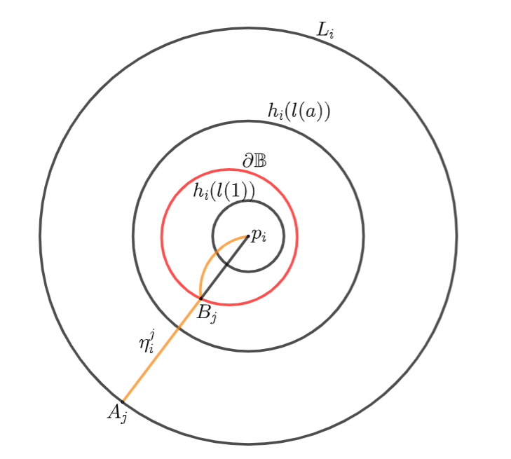
Then combining with (7), (14) and Part of Theorem 5 we have
| (15) |
which in particular tells that the four loops and are pairwisely disjoint.
Assume that the set of all tangency points on is
arranged in the anti-clockwise direction. For each , we let be the geodesic ray joining and under the hyperbolic metric . We remark here that there may exist several intersection points between and the loop . Now define to be the last intersection point between them on the direction from to , i.e., is the unique point on the ray such that
where is the subsegment of joining and . By (15) we know that where is topologically a disk. Then for any point , there exists a unique shortest geodesic joining and under the hyperbolic metric . In particular, we let be the unique shortest geodesic joining and . Now consider the concatenation (see Figure 5 for an illustration)
| (16) |
By construction, it is not hard to see that
-
(1)
for , ;
-
(2)
the curve joins and with .
Moreover, the length can be effectively bounded from above. More precisely, it follows by (2), (12) and Lemma 3 that for each and large enough,
| (17) | ||||
Assume that are two simple curves joining and certain points on such that and both and only intersect with at their endpoints. Denote by the domain enclosed by and in the anti-clockwise direction from to (see Figure 6 for an illustration).
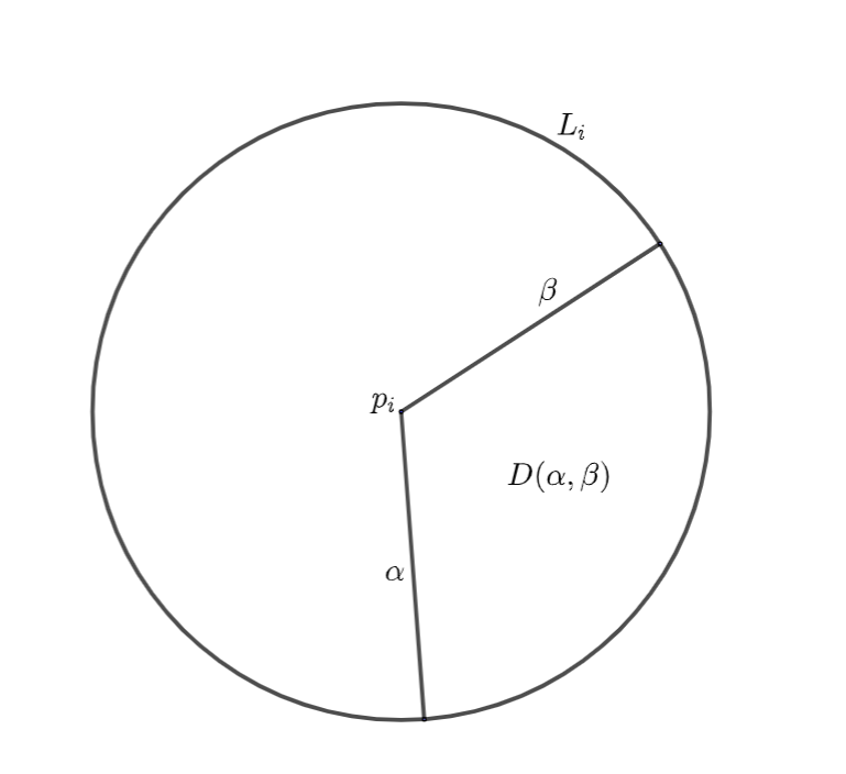
For any , for simplicity we denote
Now we give a division for each and prove the following result which is important in the proof of Theorem 1.
Lemma 6 (A division of ).
Assume that is defined in (8) and , then for large enough, there exist a positive integer with and a sequence of integers with
such that for each
| (18) |
and
| (19) |
Proof.
Recall that . First it follows from (11) and Lemma 3 that
| (20) |
Notice that . Similarly, it follows by Lemma 3 that implying
where we apply our assumption in the last inequality. Since , we have that for large enough,
| (21) |
Recall that for any , is the geodesic ray joining and under the hyperbolic metric . Then it follows from (3), (21) and Lemma 3 that for any and large enough,
| (22) | ||||
Similarly, for we also have
| (23) |
Choose an integer and a sequence of increasing integers with such that they satisfy the following three conditions:
-
(a)
;
-
(b)
for each ,
-
(c)
.
Now we prove that the and are the desired integer and sequence. First from (20) and Condition we have
| (24) |
Next it follows from (20), (22) and Condition that for each ,
| (25) |
where the second inequality holds since from (22) and Condition we have
For each , we have
| (26) | ||||
Similar as the first inequality in (22) we also have
| (27) |
Recall that . So . Then it follows by (25), (26) and (27) that for each and large enough,
| (28) |
By a similar argument, if , we also have
| (29) |
Now it remains to bound . From (25) we have
which implies that for large enough,
| (30) |
The proof is complete. ∎
4. Proof of Theorem 1
In this section, we finish the proof of Theorem 1. First we always assume that is defined in (8). For simplicity of notation, we denote
and
From Lemma 6, we have the following decomposition of :
where each small triangle is enclosed by three short horocycle segments (see Figure 7 for an illustration).
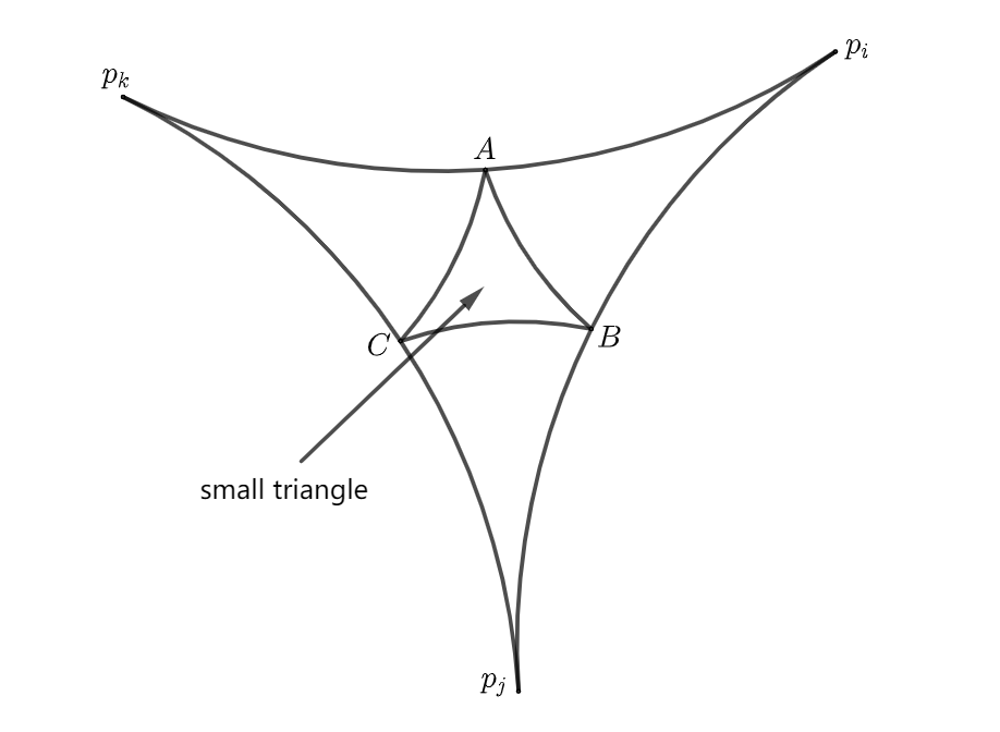
Denote
For each short horocycle segment , it uniquely determines a domain amongst
such that is contained in the boundary of . Let be a small triangle enclosed by three short horocycle segments . We say that are sector domains of . We remark here that may be the same as for .
Take two symbols and , and let be a mapping. Since
it follows that amongst , at least two of them have the same image under the mapping . We say the mapping is compatible on if
for every small triangle .
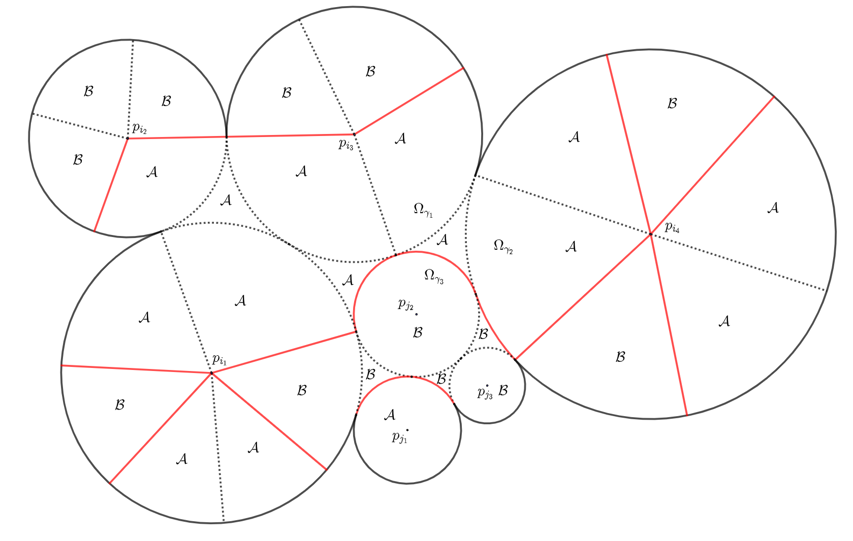
Remark.
See Figure 8, for examples:
-
(a)
if , then we have In this case both the short horocycle segments and are not contained in the boundary of and because they are interior points of .
-
(b)
If , then we have . In this case all the short horocycle segments are not contained in the boundary of and for same reason above.
Define
It is clear that is a finite set and there exists a uniform probability measure on it. For any , it will induce a division of , where
| (31) |
It is clear that the two boundaries coincide, i.e., .
Remark 7.
For a compatible mapping , it is clear that for any small triangle , at most one of its horocycle segment boundaries is contained in .
For any property , denote by the probability that a random element satisfies property , i.e.,
Here we emphasis again that the randomness is only on and the surface is fixed. For any random variable on , denote by and the expected value and variance of respectively. Now we consider the following three random variables:
-
(1)
;
-
(2)
;
-
(3)
.
We will bound the expected values of and . The first one is
Lemma 8.
For large enough, we have
Proof.
For each element , the boundary consists of two parts: the simple curves defined in (16) and certain short horocycle segments. From Lemma 6, we have that for any and ,
| (32) |
Since , by (32) we may conclude that the first part has total length . Now we estimate the total length of the second part: for any small triangle enclosed by three short horocycle segments , we denote
If , then . If exactly two of are the same, then . If are pairwise distinct, then . To summarize, we have that for any small triangle ,
It follows that
| (33) |
Recall that for any short horocycle segment ,
Combined with Remark 7, we have that for any small triangle ,
| (34) |
Since there are small triangles, together with (33), (34) and the property that the first part has total length , we obtain
as desired. ∎
Set
where , defined in (16), are the simple curves in Lemma 6. It is clear that where is the measure induced from the hyperbolic metric on . For any subset , the characteristic function is defined by
Then the expected value satisfies
where the last equality holds since for any ,
Now we calculate . By definition we have
Thus, the variance satisfies
| (35) | ||||
Recall that the Chebyshev inequality says that for any and random variable with expected value and variance , then
Now we apply the Chebyshev inequality to the case that and where is arbitrary. Since , we have
| (36) |
The following lemma is motivated by [7, Lemma 1].
Lemma 9.
For any and large enough, we have
Proof.
By (36) it suffices to show that for large enough,
| (37) |
Recall that
where
Now we split the product as the following four parts:
and
It is clear that
For any , there are four cases:
-
(1)
for some ;
-
(2)
for some and small triangle such that is not a sector domain of ;
-
(3)
for some and small triangle such that is not a sector domain of ;
-
(4)
for two small triangles and which do not share any common sector domain.
For all the four cases of above, the two events for and are independent. So we have that for any ,
| (38) |
Thus, to prove (37), from (35) it suffices to show that for large enough,
| (39) |
where is the product measure on . The proof is split into the following three sublemmas.
SubLemma 10.
For large enough, we have
Proof.
For each small triangle , it follows by Lemma 3 that
| (40) |
From (12) and Lemma 6 we know that for any and ,
By definition of we also have that for any ,
In summary, for any ,
| (41) |
Since there are small triangle and each small triangle has at most three sector domains, together with (40) and (41), we have
where runs over all pairs of small triangle and such that is a sector domain of . ∎
SubLemma 11.
For large enough, we have
Proof.
For any and , from Lemma 6 we know that the boundary contains at most short horocycle segments. For any , the boundary contains at most short horocycle segments. In summary, we deduce that for each , it has at most small triangles such that is contained in the set of sector domains of each small triangle. This implies that for each small triangle , there are at most small triangles which share at least one common sector domain with . Thus we have
where runs over all pairs of small triangles sharing at least one common sector domain. ∎
SubLemma 12.
For large enough, we have
As a direct consequence of Lemma 9,
Lemma 13.
For any and large enough,
Proof.
Then the conclusion follows by (42). ∎
Now we are ready to prove Theorem 1.
Proof of Theorem 1.
For any and let be arbitrary. Then from Lemma 8 and Lemma 13 we have that for any ,
Recall that (9) says that for large enough,
Then the conclusion follows by letting and . ∎
Remark.
In the proof of Theorem 1, a small triangle in is enclosed by three short horocycle segments each of which has length equal to . If we replace each small triangle by a geodesic triangle enclosed by three geodesic segments of lengths equal to , then the proof of Theorem 1 actually can improve to in Theorem 1. We are grateful to one referee for pointing out it to us.
We enclose this work by the following direct consequence. First recall that
Theorem.
[3, Theorem 4.1] For sufficiently large, there is a constant only depending on such that if is a punctured Riemann surface with cusps of length , then
where is the conformal compactification of .
Furthermore, as .
Corollary 14.
Let be a random element of . Then for any ,
References
- [1] G. V. Belyĭ. Galois extensions of a maximal cyclotomic field. Izv. Akad. Nauk SSSR Ser. Mat., 43(2):267–276, 479, 1979.
- [2] Béla Bollobás. The isoperimetric number of random regular graphs. European J. Combin., 9(3):241–244, 1988.
- [3] Robert Brooks. Platonic surfaces. Comment. Math. Helv., 74(1):156–170, 1999.
- [4] Robert Brooks and Eran Makover. Random construction of Riemann surfaces. J. Differential Geom., 68(1):121–157, 2004.
- [5] Robert Brooks and Andrzej Zuk. On the asymptotic isoperimetric constants for Riemann surfaces and graphs. J. Differential Geom., 62(1):49–78, 2002.
- [6] Thomas Budzinski, Nicolas Curien, and Bram Petri. The diameter of random Belyĭ surfaces. Algebr. Geom. Topol., 21(6):2929–2957, 2021.
- [7] Thomas Budzinski, Nicolas Curien, and Bram Petri. On Cheeger constants of hyperbolic surfaces. arXiv e-prints, page arXiv:2207.00469, July 2022.
- [8] Peter Buser. A note on the isoperimetric constant. Ann. Sci. École Norm. Sup. (4), 15(2):213–230, 1982.
- [9] Jeff Cheeger. A lower bound for the smallest eigenvalue of the laplacian. Problems in analysis, 625(195-199):110, 1970.
- [10] Shiu Yuen Cheng. Eigenvalue comparison theorems and its geometric applications. Math. Z., 143(3):289–297, 1975.
- [11] Alex Gamburd. Poisson-Dirichlet distribution for random Belyi surfaces. Ann. Probab., 34(5):1827–1848, 2006.
- [12] Stephen Gelbart and Hervé Jacquet. A relation between automorphic representations of and . Ann. Sci. École Norm. Sup. (4), 11(4):471–542, 1978.
- [13] Will Hide. Spectral gap for Weil-Petersson random surfaces with cusps. arXiv e-prints, page arXiv:2107.14555, July 2021.
- [14] Will Hide and Michael Magee. Near optimal spectral gaps for hyperbolic surfaces. arXiv e-prints, page arXiv:2107.05292, July 2021.
- [15] H. Iwaniec. Selberg’s lower bound of the first eigenvalue for congruence groups. In Number theory, trace formulas and discrete groups (Oslo, 1987), pages 371–375. Academic Press, Boston, MA, 1989.
- [16] Henry H. Kim. Functoriality for the exterior square of and the symmetric fourth of . J. Amer. Math. Soc., 16(1):139–183, 2003. With appendix 1 by Dinakar Ramakrishnan and appendix 2 by Kim and Peter Sarnak.
- [17] Michael Lipnowski and Alex Wright. Towards optimal spectral gaps in large genus. arXiv preprint arXiv:2103.07496, 2021.
- [18] W. Luo, Z. Rudnick, and P. Sarnak. On Selberg’s eigenvalue conjecture. Geom. Funct. Anal., 5(2):387–401, 1995.
- [19] Michael Magee and Frédéric Naud. Explicit spectral gaps for random covers of Riemann surfaces. Publ.math IHES, DOI: 10.1007/s10240-020-00118-w, 2020.
- [20] Michael Magee, Frédéric Naud, and Doron Puder. A random cover of a compact hyperbolic surface has relative spectral gap . Geom. Funct. Anal., to appear, arXiv:2003.10911, 2020.
- [21] Maryam Mirzakhani. Growth of Weil-Petersson volumes and random hyperbolic surfaces of large genus. J. Differential Geom., 94(2):267–300, 2013.
- [22] Bram Petri. Random regular graphs and the systole of a random surface. J. Topol., 10(1):211–267, 2017.
- [23] Atle Selberg. On the estimation of Fourier coefficients of modular forms. In Proc. Sympos. Pure Math., Vol. VIII, pages 1–15. Amer. Math. Soc., Providence, R.I., 1965.
- [24] Yang Shen and Yunhui Wu. Arbitrarily small spectral gaps for random hyperbolic surfaces with many cusps. arXiv e-prints, page arXiv:2203.15681, March 2022.
- [25] Alex Wright. A tour through Mirzakhani’s work on moduli spaces of Riemann surfaces. Bull. Amer. Math. Soc. (N.S.), 57(3):359–408, 2020.
- [26] Yunhui Wu and Yuhao Xue. Random hyperbolic surfaces of large genus have first eigenvalues greater than . Geom. Funct. Anal., 32(2):340–410, 2022.