equations
| (0.1) |
The bulk-edge correspondence for curved interfaces
Abstract.
The bulk-edge correspondence is a condensed matter theorem that relates the conductance of a Hall insulator in a half-plane to that of its (straight) boundary. In this work, we extend this result to domains with curved boundaries. Under mild geometric assumptions, we prove that the edge conductance of a topological insulator sample is an integer multiple of its Hall conductance. This integer counts the algebraic number of times that the interface (suitably oriented) enters the measurement set. This result provides a rigorous proof of a well-known experimental observation: arbitrarily truncated topological insulators support edge currents, regardless of the shape of their boundary.
1. Introduction and Main results
1.1. Introduction
The study of topological insulators is a central topic in condensed matter physics. These materials are insulating phases of matter, described by a Hamiltonian with a spectral gap, to which one can associate a quantized topological invariant: the Hall conductance. When two insulators with distinct topological invariants are glued together, protected gapless currents emerge along the interface: the material becomes a conductor. For straight interfaces, the interface conductance is also quantized and equals the difference of the bulk topological invariants. This fundamental result is called the bulk-edge correspondence.
The quantization of the bulk conductance (i.e. the fact that it takes values in a discrete set) was first observed in the quantum Hall effect [L81, TKNN, H82]. The characterization of Hall conductances as a Chern number marked the birth of topological phases of matter. Haldane [H88] demonstrated on a famous model of magnetic graphene that this phenomenon is not restricted to quantum Hall systems. Hatsugai [Hatsugai] then showed that topological materials support gapless states along their boundary; this is known today as the bulk-edge correspondence. Since then, the bulk-edge correspondence has been extended to various situations: see [KM05a, KM05b, FKM07] for -topological insulators, [GT18, ST19] for Floquet topological systems, and [HR08, RH08, YGS15, DMV17, PDV19, F19] for physical fields beyond quantum science, such as photonics, accounstics and fluid mechanics. By now mathematical proofs of the bulk-edge correspondence have spanned a wide variety of situations: see for instance [Hatsugai, KS02, EG02, KS04, L15, Ku17, Br18, LT22, L23] for discrete models, [EGS05, LH11, GS18, ST19] for disordered systems, [GP13, ASV13, FSSWY20] for -topological insulators, and [B19, D21b, D21, SW22a] for continuous Hamiltonians.
Various experimental results have suggested that the bulk-edge correspondence is an extremely stable principle: it does not depend on the fine details of the interface [WMTHXHW17, NHCR18, FSSWY20, TJCIBBP21]. However, with the exception of some -theoretic approaches [Ku17, LT22, L23], most proofs of the bulk-edge correspondence have focused on straight interfaces. In this work, we provide a spectral proof of the bulk-edge correspondence for curved interfaces. We show equality between the edge conductance and an integer multiple of the Hall conductance; this goes beyond the aforementioned -theoretic results where the bulk index takes the form of a geometric Hall conductance. We provide a physical interpretation of the emerging integer as an intersection number between the boundary and the measurement set. To the best of our knowledge, this is the first time that such a quantity emerges in the study of topological insulators.
1.2. Main result
We briefly review standard facts from condensed matter physics. Electronic propagation in a quantum material follows the Schrödinger equation with a selfadjoint operator on . The operator describes the hopping of the electron between atomic sites. Its spectrum characterizes the electronic nature of the material: is a conductor at energy if and only if ; and an insulator otherwise. In this paper, we will work with Hamiltonians that model limited hopping:
Definition 1 (ESR).
We say that a selfadjoint operator on is exponentially-short-range (ESR) if its kernel satisfies, for some ,
| (1.1) |
In (1.1), denotes the -distance between . When is an insulator at a certain energy, we can compute an invariant that characterizes the topological phase described by : the Hall conductance. It is the intrinsic conductance of the material originating from the quantum Hall effect, see [TKNN].
Definition 2 (Hall conductance).
Let be an ESR Hamiltonian with a spectral gap , and be the spectral projection below energy : . The Hall conductance of in the gap is:
| (1.2) |
The gap condition ensures that (1.2) is well-defined; see e.g. [EGS05] (or Proposition 1 below). This work aims to prove the bulk-edge correspondence: for edge systems interpolating between two insulators, the conductance of the edge is equal to the difference between the two Hall conductances. We turn to the definition of edge systems:
Definition 3 (Edge operator).
Let be two ESR Hamiltonians and . An edge Hamiltonian associated to and in and is a selfadjoint operator on that satisfies the kernel estimate:
| (1.3) |
The condition (1.3) means that describes two insulators glued along the edge . To measure the conductance of along , we now discuss sets transverse to .
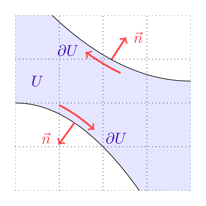
Definition 4 (Transversality).
We say that two sets are transverse if
| (1.4) |
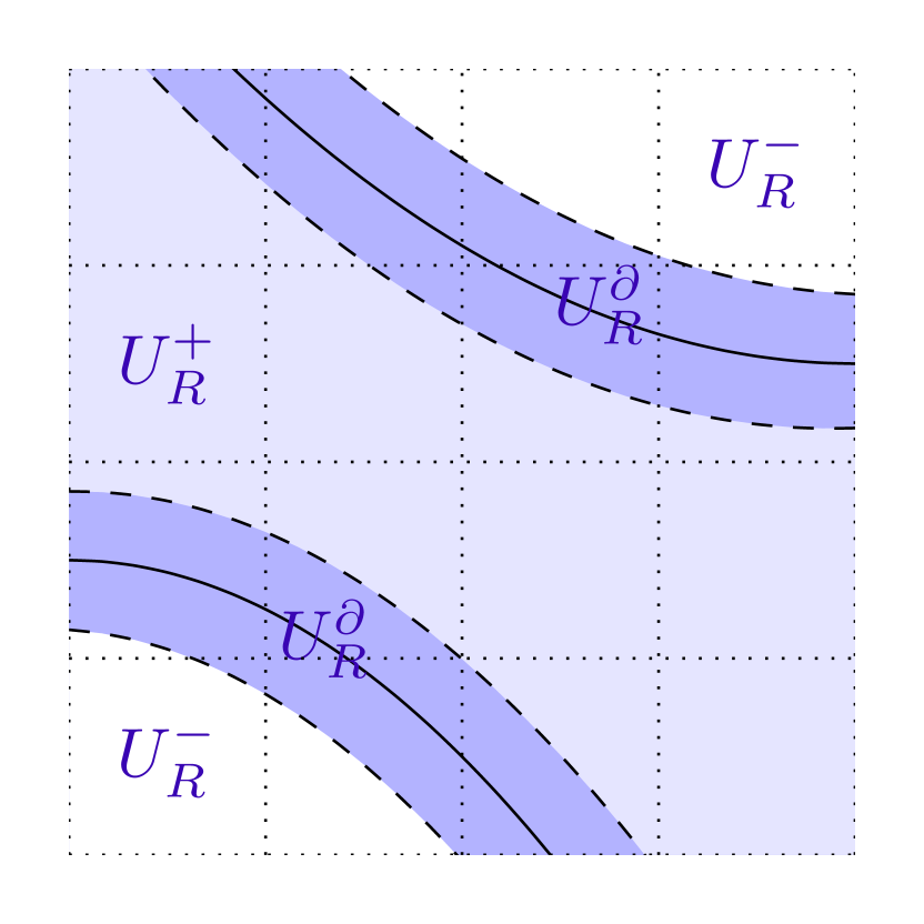
In (1.4), denotes the -distance between and the set . Transversality is a geometric condition on the relative position of the boundaries and . It demands that these two sets get away from each other at a relatively mild rate, typically for some . Under the transversality condition (1.4), we can define the conductance of along into the measurement set :
Definition 5 (Edge conductance).
Let be an edge operator associated to two Hamiltonians with a joint spectral gap , in the sets . Assume that are transverse. The edge conductance of into for energies in the bulk spectral gap is:
| (1.5) |
where is a function such that:
| (1.6) |
In (1.5), measures the number of particles moving into the set per unit time, while is an energy density in . As a result, captures the expected charge moving along into per unit time and per unit energy: it is the conductance of along . Transversality of guarantees that is well defined; see Proposition 3 below. We also mention that does not depend on satisfying (1.6) – this follows, for instance, from Theorem 1 below. Definitions 1 - 5 serve as the basis for our setup:
Assumption 1.
In this work:
-
(1)
are two selfadjoint ESR operators on with a joint spectral gap ; are the spectral projectors below energy .
-
(2)
are transverse subsets of .
-
(3)
is an edge Hamiltonian associated to in .
We are now ready to state our main result:
Theorem 1 (Bulk-edge correspondence).
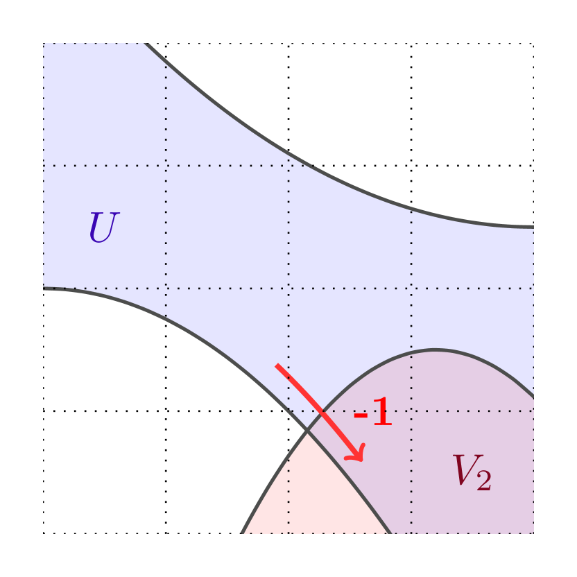
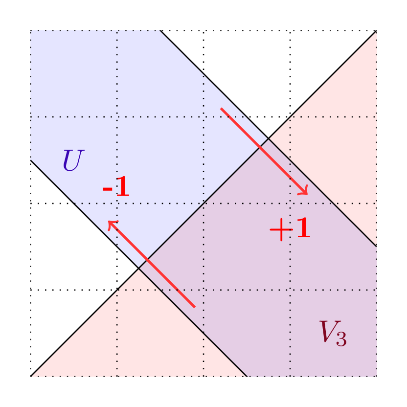
In rough terms, the integer emerging in the formula (1.7), which we call the intersection number, counts algebraically how many times the boundary of (suitably oriented) enters . See Figures 1 and 2 for a brief description on how to compute and §5.1, §LABEL:sec-7.2 for detailed definitions.
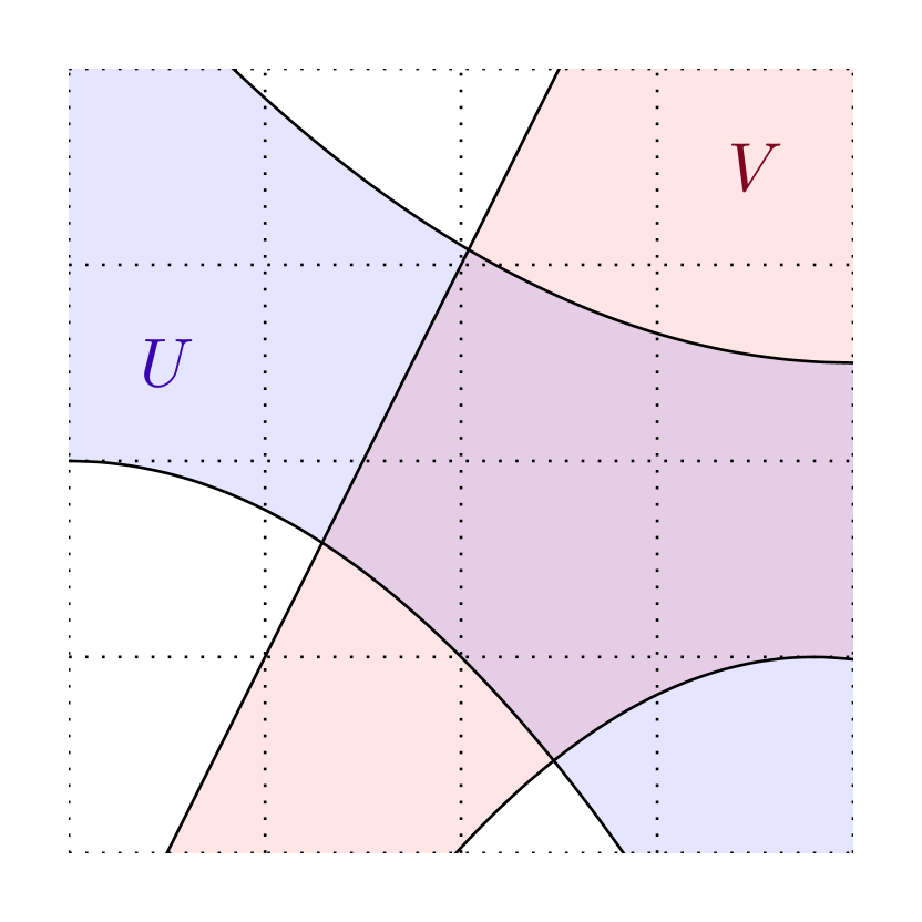
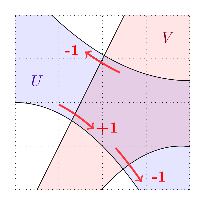
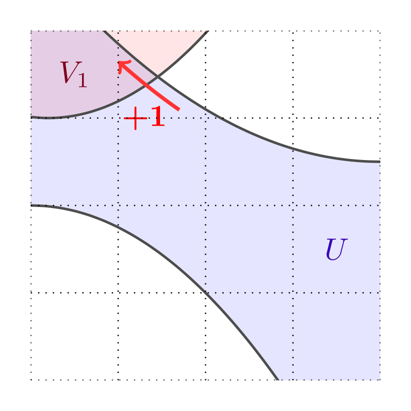
Theorem 1 is a version of the bulk-edge correspondence that goes beyond half-planes: it applies to sets with arbitrary geometry. In particular, leveraging flexibility on improves our knowledge on edge currents. When is disconnected, our result shows that each connected component of supports a current with conductance , propagating according to the orientation of ; see Figures (2(a)) and (2(b)). Another application is when is a strip and is perpendicular to : Theorem 1 implies that the edge conductance vanishes since the intersection number is ; see Figure (2(c)). Both these facts were heuristically known but rigorous proofs were missing.
1.3. Sketch of Proof
Our proof of Theorem 1 consists of two independent components.
Part 1 (§2-§4). This part reduces the edge conductance to a bulk quantity (i.e. that depends only on , ). The key observation is that one can formally think of as a singular trace:
| (1.8) |
We call it “singular” because the operator is not technically trace-class. However, if is a -tubular neighborhood of then is trace-class, and algebraic manipulations show that this trace vanishes. Therefore, as singular traces,
| (1.9) |
which is essentially a bulk term: for , depends essentially on the bulk Hamiltonians and .
At the heuristic level, our proof is based on the above informal observation but its mathematical execution is more sophisticated. We follow a strategy due to Elgart–Graf–Schenker [EGS05], tailored to the more complex geometry under focus here. To avoid trace-class issues, we inject the cutoff in the very first step: in the formula rather than in the ill-defined quantity . Getting to the rigorous analogue of (1.9) produces commutators which we analyze using Helffer–Sjöstrand formulas and cyclicity. Edge terms vanish as predicted, and this eventually yields
| (1.10) |
see Theorem 2 below. We call the emerging qauntities geometric bulk conductances.
Part 2 (§5-§LABEL:sec-7). In this part we reduce the geometric bulk conductances to integer multiples of Hall conductances (see Theorems 3 and LABEL:thm:2 below); we give an interpretation of the emerging integer as an intersection number between and . The key observation is that is the trace of a commutator where and are not separately trace-class:
| (1.11) |
In particular, a compact perturbation of does not affect , because
| (1.12) |
where the last identity comes from cyclicity, see Proposition 2 below.
When and are simple sets (i.e. their boundaries are connected), our strategy consists of using the robustness of the geometric bulk conductance to locally deform and to half-planes and recover the Hall conductance. In details, we construct sets , , that (up to permutation of and ) resemble , in (the disk of radius , centered at the origin) and , outside . Since , resemble , outside , the robustness of geometric bulk conductances (Proposition 2) guarantees that
| (1.13) |
On the other hand, , approach , when for every . So formally,
| (1.14) |
The main challenge is to make (1.14) rigorous. We will rely on an application of the dominated convergence theorem on specifically designed deformations of . Because (1.11) is a trace, the involved kernel is negligible outside large enough balls. Our construction of preserve this negligibility uniformly, and this yield a rigorous proof of (1.14) for simple sets ; see Proposition 5.
In §LABEL:sec-7 we will use additivity properties of the bulk conductances to extend (1.14) to arbitrary transverse sets , driving the emergence of the intersection number between and :
| (1.15) |
See Theorem LABEL:thm:2. Theorem 1 will follow from combining (1.10) and (1.15).
The paper is organized as follows:
1.4. Relation to existing results
The bulk-edge correspondence has been extensively studied in the past thirty years. Various perspectives have been developed around it: -theoretic approaches [KS02, KS04, T14, PS16, BKR, Ku17, Br18]; spectral flow methods [Hatsugai, Br18]; and tracial techniques [EG02, EGS05, GP13, GS18, GT18, ST19, B19, D21].
While many papers have focused on extending the bulk-edge correspondence to increasing degree of generality on the model – from Landau Hamiltonian to -insulators, from discrete to continuous, from periodic to disordered – very few go beyond straight edges. The work [BBDKLW23] gave an explicit formula for edge states of an adiabatically modulated Dirac operator with a weakly curved interface. The result relies on semiclassical methods and gives precise results but is restricted to the adiabatic regime; see also [D22, B22, PPY22]. Our previous work [DZ23] shows the emergence of edge spectrum for topological insulators as long as both the domain and its complement contain arbitrarily large balls, but did not provide a formula for the conductance. Thiang [T20] derived similar results using -theory and coarse geometry.
Later in [LT22, L23], Ludewig and Thiang proved a K-theoretic version of the bulk-edge correspondence on flasque spaces. These are spaces that satisfy coarse-geometric properties; in contrast with our condition (1.4), flasqueness [R96, Definition 9.3] can be challenging to check on concrete examples beyond perturbations of half-spaces. Their K-theoretic bulk-edge correspondence result [L23, Theorem V.4] and edge-traveling interpretation [L23, Theorem VII.7] together connect the edge conductance to the geometric bulk conductance (1.10). Our approach goes beyond [LT22, L23] by connecting the geometric conductances themselves to a topological marker independent of the geometry: the Hall conductance (1.2). This drove the emergence of the intersection number .
1.5. Open problems
One natural question is whether our curved bulk-edge correspondence (1.7) holds for -topological insulators. This would require a space-based trace formula for -bulk indices, such as (1.2) for Hall insulators. At this point it is unclear whether such a formula is available or even possible; see for instance discussions in [LM19, FSSWY20].
Another interesting problem concerns the type of the edge spectrum; it is widely expected to include an absolutely continuous part. For instance, [BW22] proved that the edge spectrum is filled with absolutely continuous spectrum when the edge is straight, combining a form of the bulk-edge correspondence derived in [FSSWY20] with a result on the structure of unitary operators [MM21]. The present work provides the first step in the context of curved edges. In a follow-up project we will show that the emerging edge spectrum is absolutely continuous, extending the result of [BW22].
In [CB23], Chen and Bal showed that for a straight edge, the bulk index is equal to the difference between the number of modes reflected and transmitted. It would be very interesting to extend this result to curved edges. Yet this promises to be challenging, because the scattering techniques developed there rely on translational invariance.
Several authors [HM15, GMP17, BBDF18] have shown that the Hall conductance of interacting systems of particles is quantized (i.e. takes values in a discrete set). In our proof a geometric bulk conductance naturally emerges, see (1.10); it would be interesting to investigate whether the analogue of this quantity in interacting systems is quantized as well, and given by the integer times the Hall conductance.
1.6. Funding and/or competing interests
We gratefully acknowledge support from the National Science Foundation DMS 2054589 (AD) and the Pacific Institute for the Mathematical Sciences (XZ). The contents of this work are solely the responsibility of the authors and do not necessarily represent the official views of PIMS.
1.7. Notations
We use the following notations:
-
•
Regular font , , denotes scalars in , , or .
-
•
Bold font denotes points in .
-
•
denote the Euclidean metric.
-
•
denote the -metric on .
-
•
denote the logarithm metric on .
-
•
and denote the operator norm and the trace-class norm, respectively.
-
•
Throughout the paper, denotes a constant that is allowed to vary from line to line, that may depend on and (though this dependence is not emphasized). We will occasionally use to emphasize dependence on an integer .
-
•
For , denotes the open set .
-
•
denotes the -disk centered at , of radius .
-
•
and .
-
•
If is an operator on , denotes the Schwartz kernel of .
2. Preparation
In this section, we give some basic operator estimates that will be needed but leave the proof to Appendix LABEL:app-ESR.
2.1. Operator estimates
Under short-range assumptions, we give here estimates on resolvents and product of operators. We start by introducing the notion of textitpolynomially-short-range (PSR) Hamiltonians.
Definition 6 (PSR).
An operator on is polynomially-short-range (PSR) if for any , there is such that
Note that any ESR operator is also PSR. The next result shows that (1) resolvents of ESR for insulating energies are ESR; (2) functionals of ESR operators are PSR.
Lemma 2.1.
Assume is self-adjoint and ESR.
-
(a)
For , is ESR. More precisely,
(2.1) -
(b)
For any , is PSR.
We now give estimates on products of ESR / PSR operators. We state them in a unifying way using the two metrics .
Lemma 2.2.
Let . Let be a selfadjoint operator on that satisfies the kernel estimate
Then
| (2.2) | |||
| (2.3) | |||
| (2.4) |
Lemma 2.3.
Let . Assume that are self-adjoint operators on that satisfy the following estimates:
{equations}
∀j ∈[1,n], —S_j(x, y)—≤C_j e^-cd_*(x, y);
∃p ∈[1,n], —S_p(x, y)—≤C_p e^-cd_*(x, y) - cd_*(x, ∂U ) - cd_*(y, ∂U );
∃q ∈[1,n], —S_q(x, y)—≤C_qe^-cd_*(x, y) - cd_*(x, ∂V ) - cd_*(y, ∂V).
Then we have
| (2.5) |
where , .
Note that is independent of and
| (2.6) |
2.2. Transversality and trace-class
Recall that we say if
| (2.7) |
Note that it is equivalent to
| (2.8) |
Meanwhile, because of the inequality
we have:
| (2.9) |
Therefore for any , by (2.8)
| (2.10) |
The next result states that product of PSR operators that decay away from the boundaries of transverse sets are trace-class.
Corollary 2.4 (trace-class).
Assume are transverse sets. Assume , , are PSR and for some and for any , there is such that
Then is trace-class.
3. Bulk and edge conductance
From now on, we always assume that Assumption 1 holds.
In this section, we show that the Hall conductance (1.2), the geometric bulk conductance (1.10), and the edge conductance (1.5), are well-defined.
3.1. Geometric bulk conductances
Proposition 1.
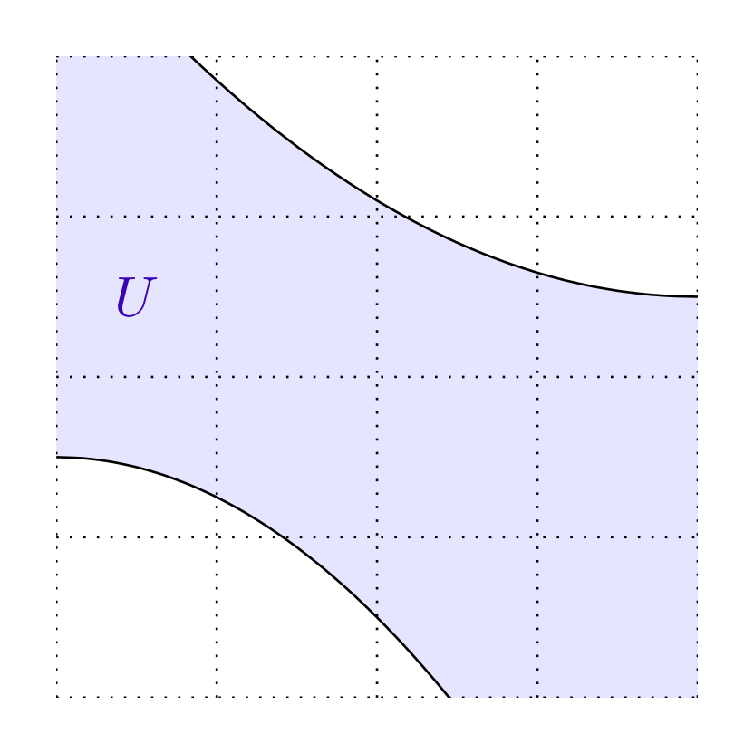
Because the right and upper half-planes are transverse sets, the Hall conductance is well-defined.
Proof.
Since is a spectral gap, for any , the spectral projectors and are equal. This proves independence.
We then show that is well-defined. Without loss of generalities we may assume that is an interval; pick as the midpoint and such that . By Lemma 2.1(a), is PSR (one can actually prove that it is ESR). By (2.4), for any , there exists such that
| (3.2) |
Introduce
| (3.3) |
| (3.4) |
Since are transverse subsets of , by Corollary 2.4, is trace-class; thus is well-defined. This completes the proof. ∎
Given two sets , we introduce the symmetric difference
| (3.6) |
One of the key properties of geometric bulk conductances is:
Proposition 2.
[Robustness of geometric bulk conductances] Under Assumption 1, assume is such that for some ,
| (3.7) |
Then .
Proof of Proposition 2.
First, are transverse and are well-defined. Indeed, by (2.9) and (3.7),
for any and large enough . Hence are transverse sets and is well-defined. It remains to show:
By direct expansion of definition (3.1) and , we get
Recall the cyclicity of trace-class operators – see e.g. [K89, Proposition 7.3]:
| (3.8) |
Let us first assume that every operator below is trace-class so we can freely use cyclicity above. We get
where we used .
Now we prove every operator mentioned above is trace-class. Note that , and recall that is PSR (see the proof of Proposition 1). By (2.4),
Meanwhile, . Hence
Therefore by Corollary 2.4, and are both trace-class. Meanwhile, by (2.3) of Lemma 2.2 and , hence
By (2.10),
Hence , and similarly , are also trace-class. This completes the proof. ∎
3.2. Edge conductance
Now we can introduce the edge conductance.
Proposition 3 (Edge conductance).
For the rest of the paper, we consider an arbitrary but fixed pair of transverse sets in and omit the superscripts from for convenience.
Proof of Proposition 3.
1. By definition, ; hence . Therefore, we have:
| (3.10) | ||||
| (3.11) |
2. We now estimate . By Helffer-Sjöstrand formula (LABEL:eq:_HS_1), we have
| (3.12) |
Note that
And we have the following estimates:
Note that all the decay rate in the above bounds can be relaxed to because and . Denote . Since , we have
| (3.14) | ||||
| (3.15) |
By (2.5) in Lemma 2.3 and (2.6),
As a result, using almost analyticity (LABEL:eq:_HS_1), when , let ,
| (3.16) | ||||
| (3.17) | ||||
| (3.18) |
When , . Therefore, at the cost of potentially increasing , we have for any :
| (3.19) | ||||
| (3.20) |
4. Equality
Theorem 2.
Under Assumption 1,
| (4.1) |
Proof.
We follow an approach due to Elgart–Graf–Schenker [EGS05], tailored here to our geometic setup. Define
and correspondingly,
| (4.2) |
This quantity plays an intermediate role in proving equality (4.1). In fact, we prove (4.1) by proving the following three equalities:
| (4.3) |
As explained in §1.4, to prove Claim 1, we inject a cutoff near and justify that terms away from are negligible. Claim 2 reduces this near- edge quantity, , to the difference of two bulk quantities, . Claim 3 deform the bulk quantities, (in the limit), to the geometric bulk conductances, .
Now we state and prove these three claims.
Claim 1.
Proof of Claim 1.
Since , we split into two parts:
| (4.4) |
We show that is trace-class and that when . By (3.25), we have
| (4.5) | ||||
| (4.6) |
where we used and . Because of (3.26) and (4.6), Corollary 2.4 implies that is trace-class. We now estimate its trace. By (3.26) and (2.5) in Lemma 2.3, we get
| (4.7) |
As a result,
By (2.10), the sum is finite for . It follows that as .
It remains to prove . Without loss of generalities, – see e.g. [D21, (2.3.5)]. Combining the Helffer–Sjöstrand formula (LABEL:eq:_HS_1) with integration by parts, we obtain
| (4.8) | ||||
| (4.9) | ||||
| (4.10) |
If , then . Thus for any ,
| (4.11) |
Combining with (3.26) and using Corollary 2.4, we see that is trace-class. Using , we have:
| (4.12) |
Therefore, we can take the trace on both sides of (4.10) and switch trace and integral (using almost analyticity of ). This yields:
| (4.13) |
By (3.26), (4.11), and Corollary 2.4, the operators below are all trace-class. Thus we can apply cyclicity (3.8) to get
where we used Helffer-Sjöstrand formula (LABEL:eq:_HS_1) for the last equality. Finally,
as , , and are all trace-class by Lemma 2.1(b) and Corollary 2.4. Thus we get ; this completes the proof of Claim 1. ∎
Claim 2.
We have:
| (4.14) |
Proof of Claim 2.
Recall that . Since , from the definition (4.2), we get . To show (4.14), it is enough to show
| (4.15) |
Denote . We have:
| (4.16) | ||||
| (4.17) |
We rewrite
| (4.18) |
Note that:
Note that each , contains , and . By , , above, the control of the resolvent norm provided by Lemma 2.1(a) and (2.5) in Lemma 2.3, we have
where we used and . Therefore,
Since are transverse sets, when , by (2.10), we obtain:
By almost analyticity,
It suffices to go back to (4.17) and take to obtain (4.15). This completes the proof. ∎
Claim 3.
For any ,
| (4.19) |
Proof of Claim 3.
Note that and . By Proposition 2,
Hence we get the second equality in (4.19). WLOG we prove below. Recall that
| (4.20) |
Expand and use , we get
By the Helffer-Sjöstrand formula (LABEL:eq:_HS_1), we have
| (4.21) |
To conlude, we adapt a trick from [EGS05].
Lemma 4.1.
We have .
Proof.
By functional calculus,
Since while , is the almost analytic extension of , . Hence , and thus the whole integrand, denoted as , is analytic on . Choose large enough such that . By Stokes theorem,
A similar computation gives
However, when ,
Hence
This completes the proof. ∎
∎
5. Intersection number between simple transverse sets
In this section, we define an intersection number between simple transverse sets (see Definition 8). This integer will emerge when expressing geometric bulk conductances in terms of Hall conductances: see Theorem 3 below.
Definition 7 (Simple path).
A continuous map is called a simple path if:
-
(i)
is injective and proper (the preimage of a compact set is compact);
-
(ii)
There exists a discrete closed set such that is smooth on ;
-
(iii)
For all , the left and right derivatives of at exist and have norm .
If (ii) and (iii) hold but is periodic and injective over its period, we call a simple loop.
Proposition 4.
Let be two simple paths with ranges , such that is compactly supported. Let be a connected component of . Then there exists a unique connected component of such that is bounded.
[\capbeside\thisfloatsetupcapbesideposition=right,center,capbesidewidth=0.6]figure[\FBwidth]

Proposition 4 has a flavor reminiscent of the Jordan curve Theorem. While visually obvious (see Figure 4), its proof requires some work. We give a sketch here and defer the proof to Appendix LABEL:app:A:
-
•
We show that if is a proper injective curve, then has two connected components (Lemma LABEL:lem:4);
-
•
We then justify that a perturbation of on a compact set perturbs the two connected components by a bounded set only (Lemma LABEL:lem:5);
-
•
We unambiguously define the left side of a simple path (Proposition LABEL:prop:1) and justify that the left components of , have bounded symmetric difference (see Figure 5 for a pictorial representation and Proposition LABEL:prop:1 for a proper definition of the left of a simple curve).
[\capbeside\thisfloatsetupcapbesideposition=right,center,capbesidewidth=0.6]figure[\FBwidth]

Definition 8 (Simple set).
An open subset of is simple if it is connected and its boundary is the range of a simple path or of a simple loop.
Associated with the distinction between simple paths and simple loops, there are two types of simple sets: those with bounded boundaries (given by simple loops) and those with unbounded boundaries (given by simple paths). By Jordan’s theorem, those with bounded boundaries are bounded or have bounded complements.
5.1. Intersection number
Definition 9 (Intersection number for simple sets).
Let be transverse sets such that is simple. If is unbounded, let be a simple path with range , such that lies to the left of (see Figure 5 for a pictorial representation and Proposition LABEL:prop:1 for a proper definition). We define the intersection number between as:
| (5.1) |
If is bounded, we set .
We show in Appendix LABEL:app:B that is correctly defined and independent of the choice of curve describing its boundary. In §LABEL:sec-7.2 we extend Definition 9 to more general transverse sets , such that (loosely speaking) is made of well-separated curves.
6. Bulk index computation
6.1. Theorem 3 for transverse simple sets
The main theorem here is:
Theorem 3.
Under Assumption 1, we have
| (6.1) |
6.2. Steps 1 and 2
Lemma 6.1.
Let be transverse simple sets such that , and be an ESR projector. Then .
Proof.
We recall the notation .
1. Assume first that is bounded. Since is a simple set, by definition, is a simple loop. Hence either or is bounded by Jordan’s theorem. In the former case, Proposition 2 implies . In the latter case, Proposition 2 implies . Therefore we assume is unbounded in the rest of the proof.
2. Since , ; potentially replacing by we may assume that . Hence when is large enough, . Given , define
When , we have .
3. By continuity of distance function, and . As a result,
By (2.9),
| (6.2) | ||||
| (6.3) |
On the other hand, if , then there is such that , by definition this implies . But is an open set so . We get a contradiction; thus . In particular, for any ,
As a result, by (2.9),
| (6.4) |
Interpolating between (6.3) and (6.4) gives:
| (6.5) |
Lemma 6.2.
Let be an ESR projector. Assume that for all transverse simple sets such that , we have . Then for all transverse simple sets such that , we have .
Proof.
Assume that . Then, , and so by assumption we have . But since , we deduce that .∎
Therefore, it remains to prove that Theorem 3 holds for pairs such that .
6.3. Uniformly transverse families
Recall that transversality condition (1.4) is equivalent to (2.8):
| (6.8) |
When (6.8) holds, we refer to as -transverse.
Definition 10 (Uniformly transversality).
Let be a family of transverse simple sets. We say that is uniformly transverse if there exists such that for all , is -transverse. We say that is equivalent to if for all , and are bounded.
Uniform transversality boils down to (6.8) holding uniformly in :
| (6.9) |
Recall that , denote the right/upper half-plane.
Our strategy to prove Theorem 3 goes as follows. We will construct a family of uniformly transverse sets (see Proposition 5 and §6.5) such that are compact perturbations of and they look like inside the disk . Because are compact perturbations of , we will have by the robustness of geometric bulk conductance (Proposition 3). Meanwhile, since look like and in , we will show converges to as by showing
-
•
as for each (Lemma 6.3);
-
•
the convergence is uniform because of uniform transversality.
This will prove that converges as to , and in particular .
Lemma 6.3.
Assume that is a family of transverse sets in such that for all , and . Then for any :
| (6.10) |
Lemma 6.3 means that the geometric bulk conductance can be computed locally. This observation was key to the work [DZ23] on emergence of edge spectrum for truncated topological insulators.
Proof.
1. Recall that (3.3) satisfies the kernel estimate (3.4):
| (6.11) |
Since is linear in and , we have
Note that
Hence we have
| (6.12) |
The same estimate holds for . Hence we obtain
| (6.13) |
2. We now apply (6.13) to the pair , then to the pair : {equations} — K_U_n,V_n(x,x) - K_U_n ∩D_n(0),V_n ∩D_n(0)(x,x)—≤C_N(1 + n)^-N e^Nd_l(x, 0), {equations} — K_H_2, H_1(x,x) - K_H_2 ∩D_n(0),H_1 ∩D_n(0)(x,x) — ≤C_N(1 + n)^-N e^Nd_l(x, 0) . Because and , summing these two bounds gives {equations} — K_U_n ,V_n(x,x) - K_H_2, H_1(x,x) — ≤2C_N(1 + n)^-N e^Nd_l(x, 0) . It suffices to take the limit as goes to to conclude. ∎
Proposition 5.
Let be transverse simple sets in such that . There exists a family with the following properties:
-
(a)
is uniformly transverse;
-
(b)
is equivalent to ;
-
(c)
In the disk , is the upper half-plane and is the right half-plane .
Proposition 5 is the key construction in the proof of Theorem 3 and we defer its proof to §6.4 - §6.5.
Proof of Theorem 3 assuming Proposition 5.
By Proposition 5, there is a family satisfying (a), (b), (c) above. Since is equivalent to and , are bounded, by Proposition 2, we deduce that for all . In particular,
| (6.14) |
Our plan is now to apply the dominated convergence theorem to the above series.
6.4. Ordering entrance / exit points
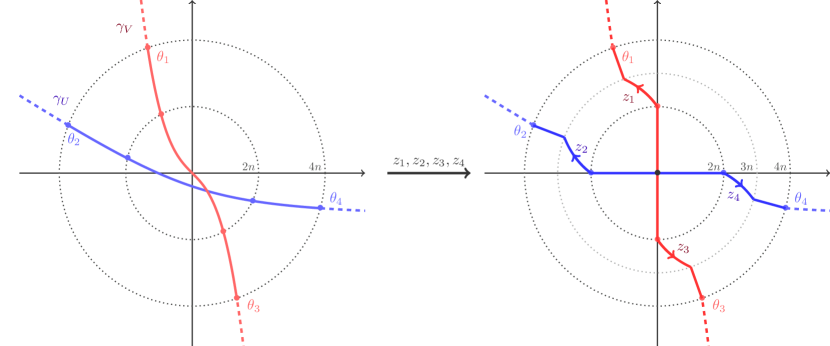
In the following two subsections, we aim to prove Proposition 5. Let be transverse simple sets. For , , define: {equations} t_J^+(r) =def sup{ t : γ_J(t) ∈¯D_r(0) }, t_J^-(r) =def inf{ t : γ_J(t) ∈¯D_r(0) }, z_J^±(r) =def γ_J ∘t_J^±(r).
Lemma 6.4.
Let be transverse simple sets such that . Let such that . For all , there exists (see Figure 6), such that
| (6.18) |
[\capbeside\thisfloatsetupcapbesideposition=right,center,capbesidewidth=0.6]figure[\FBwidth]

Proof.
1. Fix . Define
| (6.19) |
These are connected sets which do not intersect . In particular they lies in or in . But since , for sufficiently large . It follows that . Likewise .
2. Let such that ; let such that . Let be the curve defined by:
| (6.20) |
where we use the symbol to denote the concatenation of two curves. See Figure 7. Let the connected component of to the left of . The function runs clockwise. Therefore (e.g. by considering a sufficiently small disk centered at , , simply split by ) we see that lies in the component of to the right of , in particular it does not intersect .
3. Note that is an unbounded connected subset of . Because is bounded (see Proposition 4) intersects . Moreover, it does not intersect , so we have . In particular,
| (6.21) |
Because , we obtain
| (6.22) |
Therefore, for some .
[\capbeside\thisfloatsetupcapbesideposition=right,center,capbesidewidth=0.6]figure[\FBwidth]

4. By a similar argument, lies in the component of to the right of . Because does not intersect and , we deduce that as in (6.22) that
| (6.23) |
which implies for some . This completes the proof. ∎
6.5. Construction of uniformly transverse family of sets
Let be a -transverse pair with . Now we can construct a family of uniformly transverse sets that is equivalent to such that , .
By Lemma 6.4, when is large enough, for some , we have
| (6.24) |
For such an , we define four functions , by
| (6.25) |
and four curves (see Figure 8) by
| (6.26) |
We will make use of the following result:
Lemma 6.5.
Let . Assume that are such that . Then
| (6.27) |
Proof.
We first estimate . Without loss of generality, we can assume by choosing . Recall that by definition. By transversality, we see
Since , for any , . Recall that by definition, is monotone over . Hence we obtain
| (6.28) |
Meanwhile, by the definition of and the assumption , we have
| (6.29) |
Combining (6.28) and (6.29), we obtain
Since and when , , we see that
for any . This proves Lemma 6.5. ∎
We now deform by using as boundary functions. Specifically, we define two sets as the set lying to the left of the following boundaries (see Figure LABEL:fig:P12) – recall that and depends on , see (6.26):
{equations}
∂U_n = γ_U((-∞,t_U^-(4n))) ∪z_2([0,4]) ∪z_4([0,4]) ∪γ_U((t_U^+(4n), +∞)),
∂V_n = γ_V((-∞,t_V^-(4n))) ∪z_1([0,4]) ∪z