The bistability of curved compression ramp flows
Abstract
This paper investigates the bistability of curved compression ramp (CCR) flows. It reports that both separated and attached states can be stably established even for the same boundary conditions, revealing that the ultimate stable states of CCR flows also depend on the initial conditions and evolutionary history. Firstly, we design a thought experiment involving two establishment routes of CCR flows, constructing two distinct-different stable states, respectively. Subsequently, three-dimensional direct numerical simulations are meticulously performed to instantiate the thought experiment, verifying the existence of the bistable states. Finally, we compare the pressure, wall friction, and heat flux distributions under two stable states. As a canonical type of Shock wave-Boundary layer interactions, local CCR flows often appear on aircraft, hence the bistability will certainly bring noteworthy changes to the global aerothermodynamic characteristics, which supersonic/hypersonic flight has to deal with.
keywords:
1 Introduction
In shock wave-boundary layer interaction (SBLI) flows, separation and attachment of boundary layers are the two most typical states (Babinsky & Harvey, 2011). The ultimate stable states of a specific SBLI flow are widely considered to be unique for given inflow parameters and wall geometry, i.e., the boundary conditions. Although empirical, this understanding is still correct in most cases. However, in principle, effects of initial condition and evolutionary history of SBLIs can not be ignored, especially considering the reciprocal causation of shock wave (SW) patterns and boundary layer behaviors. An extreme question stemming from these process-dependent effects is that “can both stable separated and attached states exist for the same boundary conditions in pure SBLI flows?” The statement “pure” means that the flow is dominated by self-organized SBLIs rather than other multistable interactions, such as SW reflections (Ben-Dor et al., 2001; Tao et al., 2014). If the answer is “yes”, the corresponding bistability will certainly bring significant differences to the aerothermodynamic characteristics, which is inevitable for super/hypersonic flight. Herein, a class of pure SBLI flows, the canonical compression ramp (CR) flows, are chosen to investigate the process-dependent effects, and their bistability is reported.
Large separated CR flows, classified as type VI of SW interactions by Edney (1968), are composed of large separation bubbles and -shock patterns. As a typical wall geometry, direct CRs (DCRs, the inclined ramp directly connecting the flat plate with one apex) are investigated widely, including the interaction processes with boundary layers’ distortions near separation (Chapman et al., 1958; Stewartson & Williams, 1969; Neiland, 1969), the aerodynamic characteristics (Gumand, 1959; Hung, 1973; Simeonides & Haase, 1995; Tang et al., 2021), the vortex structures inside both the separation bubbles (Gai & Khraibut, 2019; Cao et al., 2021) and the evolving boundary layers (Fu et al., 2021; Hu et al., 2017), and the unsteadiness of the SBLIs (Ganapathisubramani et al., 2009; Helm et al., 2021; Cao et al., 2021). On the other hand, due to the potential to weaken separation, curved CR (CCR, inclined ramp connecting the flat plate with curved walls) flows have gradually attracted the attentions of researchers (Tong et al., 2017; Wang et al., 2019; Hu et al., 2020). However, as far as we know, there are few reports about the multistability of pure SBLIs in the CR flows.
The rest of this paper is organized as follows. Sec. 2 describes a thought experiment to construct two distinct-different stable CCR flows for the same boundary conditions. Sec. 3 presents the three-dimensional (3D) direct numerical simulations (DNSs) to instantiate the thought experiment and verify the CCR flows’ bistability. Conclusions follow in Sec. 5.
2 Thought experiment
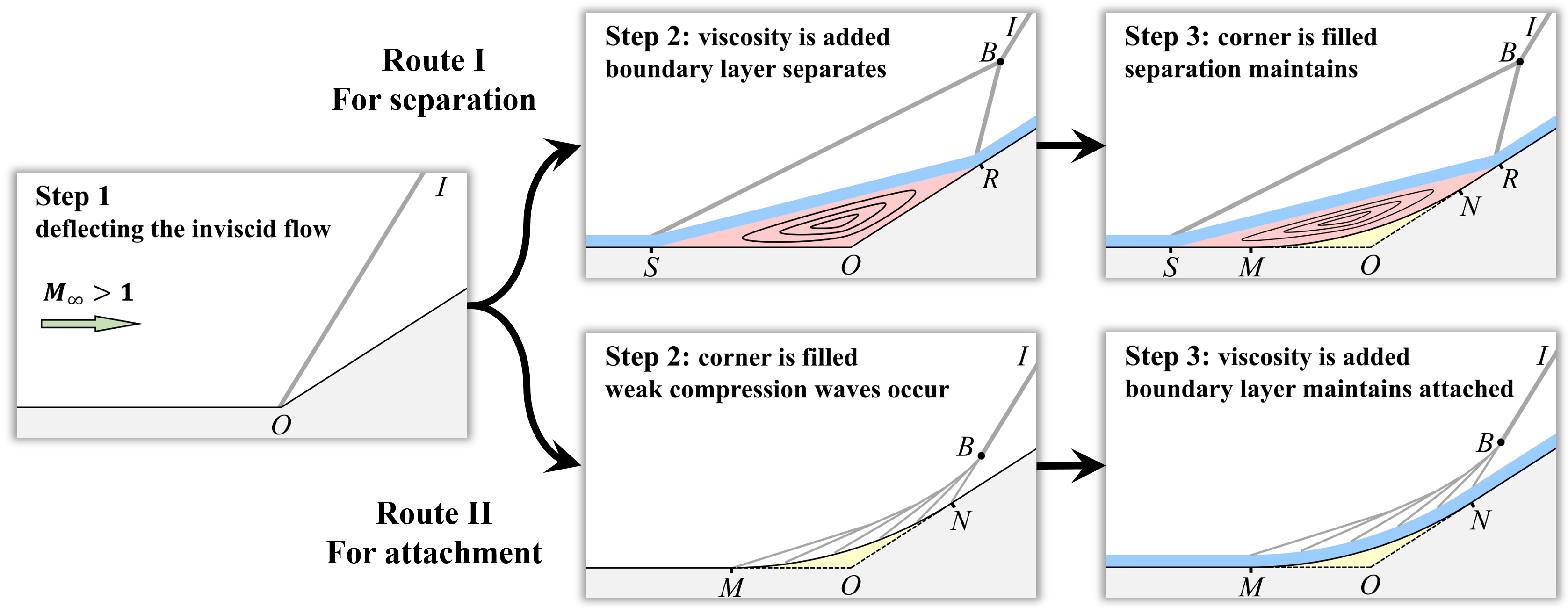
In this section, we design a thought experiment to construct two distinct-different stable CCR flows, separation and attachment, via Route I and II, respectively, as shown in Fig. 1.
First, a possible separated CCR flow is constructed via Route I with three steps.
-
•
Step 1: deflect the inviscid flow. Set the initial flow field as an inviscid supersonic flow being deflected by a DCR geometry with ramp angle . An oblique SW is formed and emits from the ramp apex ;
-
•
Step 2: add the viscosity. At some instant, the viscosity is suddenly added to the fluid. An attached boundary layer is subsequently formed and interacts with SW . For a large enough , the attached boundary layer can not resist the strong adverse pressure gradient induced by SW and then separates from the wall. The inverse flow gradually shapes a closed separation bubble , deflecting both the attached boundary layer and the outer inviscid flow, and inducing two new SWs, and . As time goes on, the separation bubble stops growing and stabilizes, i.e., both the separation point and the reattachment point become almost fixed or only oscillate slightly;
-
•
Step 3: fill the corner into an arc. The key to filling is to be slow, gentle and macroscopically continuous, ensuring that the flow is always in stable states during the filling process. Thus, we fill the corner with an ‘imaginary machine’ that can produce solid wall material atom by atom. In order to minimize the disturbance, the time span between two fillings is longer than the relaxation time of the flow stabilization. In the end, the corner is filled into an arc (the yellow region) inside space , and a stably separated CCR flow could be obtained, as shown in the end of Route I in Fig. 1.
Second, a possible attached CCR flow is constructed via Route II using three steps.
-
•
Step 1: deflect the inviscid flow. This step is the same as Step 1 in Route I;
-
•
Step 2: fill the corner into an arc. This step is similar to Step 3 in Route I, i.e., filling the corner into an arc (the yellow region). The only difference is that the corner’s filling comes before the fluid viscosity’s adding in Route II. Due to the curved wall , SW emitting from point is weakened to a series of compression waves spreading on ;
-
•
Step 3: add the viscosity. Similar to Step 2 in Route I, the viscosity is suddenly added to the fluid after the inviscid flow stably passing over the CCR in this step. Undergoing the weaker adverse pressure gradients of compression waves on , the gradually formed boundary layer is very likely to stabilize at attached state, as shown in the end of Route II.
Compare Route I and II. Operationally, both stable separated and attached CCR flows could be obtained with three steps by only exchanging the order of their last two steps. However, in essence, the different presentations of the ultimate stable states originate from the emergence history of flow elements, including the boundary layer, SWs, and compression waves. In Sec. 3, 3D DNSs are performed to check the authenticity of the thought experiment.
3 Numerical expriment
In this section, the thought experiment shown in Fig.1 is numerically instantiated using 3D DNSs. The flow field in step 1 of can be obtained with the classical Rankine-Hugoniot relations. Therefore, only four steps need to be simulated: step 2 and 3 of both Route I and II. Details of DNS are in Sec. 3.1. Route I and II are instantiated in 3.2.2 and 3.2.3, respectively. Contrast of the bistable states is in Sec. 3.3.
3.1 Details of DNSs for DCR flows
3.1.1 Governing equations and numerical methods
The governing equations solved are dimensionless 3D Navier–Stokes equations for unsteady, compressible flow in curvilinear coordinates,
| (1) |
where is the conservative vector flux, , and are the invicid convection fluxes, , and are the viscous fluxes. Here, , and are defined as
| (2) |
where are the metric coefficients and is the determinant of the Jacobian matrix transforming the Cartesian coordinates into the computational coordinates . The velocity vector , the heat flux vector and the stress tensor are defined as
| (3) |
The total energy is defined as
| (4) |
The other four flux terms have the similar forms: and are similar in form to ; and are similar in form to . The viscosity is determined with the Sutherland’s law, and perfect gas equation, relating the pressure the density and the temperature , is used to close the equations set. The Prandtl number and the specific heat ratio are chosen in the simulations. The non-dimensional variable are normalized using the inflow parameters: , , , , , and . The reference length is chosen as mm.
In terms of the numerical methods, the time integration is performed by the third-order TVD-type Runge–Kutta method; the inviscid fluxes are discreted by the fifth-order WENO method (Jiang & Shu, 1996); the viscid fluxes are discreted with the sixth-order central difference scheme. The DNSs are conducted with the in-house code OPENCFD-SC, whose capability has been well examined (Hu et al., 2017; Xu et al., 2021), especially in studying compression ramp flows.
3.1.2 Wall geometry, flow parameters, mesh spacing and initial & boundary conditions
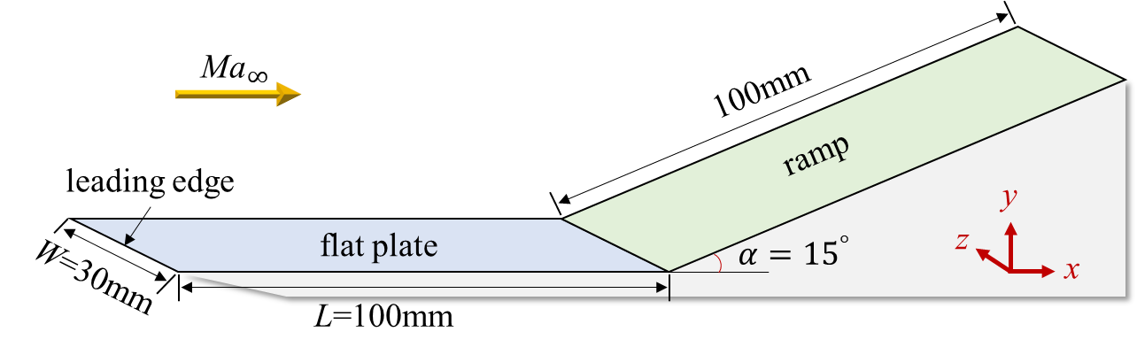
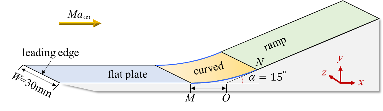
The choices of the compression ramp geometry (DCR) and the flow parameters are based on the recent shock-tunnel experiments (Roghelia et al., 2017a, b; Chuvakhov et al., 2017). As the DCR configuration shown in Fig. 2, the DCR configuration is mainly composed of two parts, the flat plate and the ramp, both of which have the same length mm and width mm. The ramp angle is . The flow parameters are shown in Tab. 1, including the Mach number , the Reynolds number , the velocity , the density , the temperature and the pressure . The isothermal wall condition is used with , since the run time of the shock tunnel is very short.
| (mm-1) | (MJ kg-1) | (m s-1) | kg m-3 | (K) | (Pa) | (K) | ||
| 0.021 |
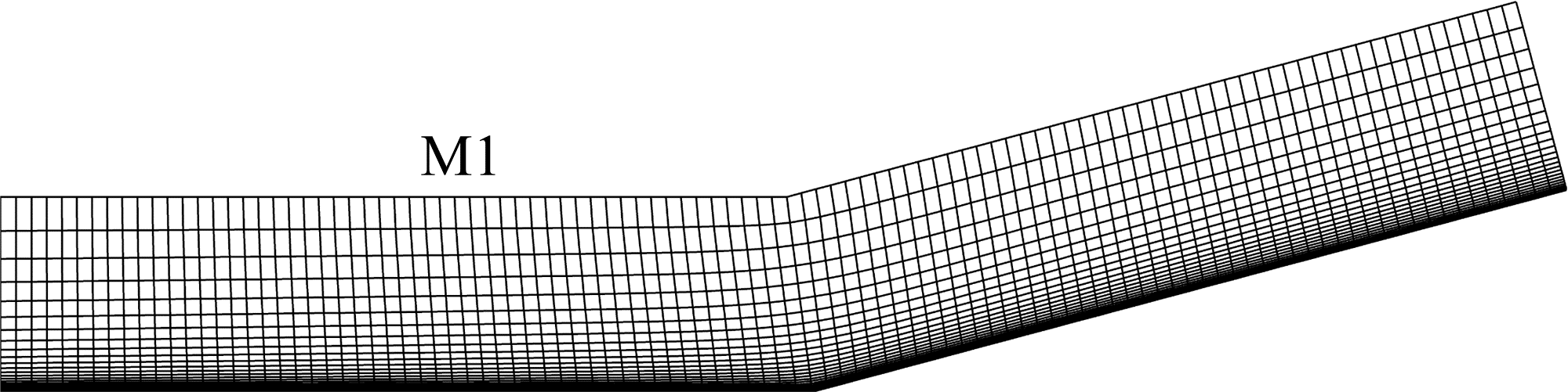
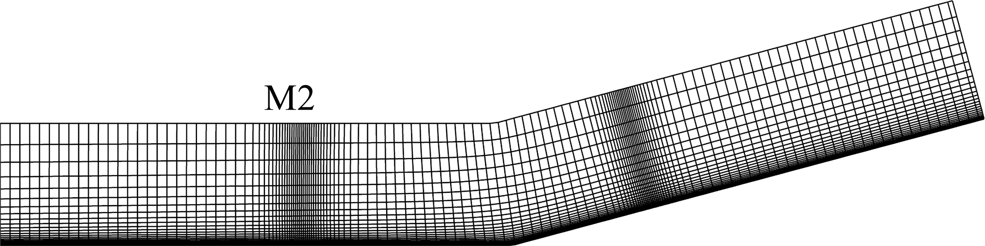
The computational domain, i.e., the mesh region, is shown in Fig. 3. The streamwise region is (the leading edge is at mm); the wall-normal height is mm; the spanwise width is mm. Two mesh resolutions, (M1) and (M2), are considered for time and grid convergence studies. Both M1 and M2 cluster the grids near the wall with the first wall-normal grid height being fixed to mm, yielding the non-dimensional height mm at . Spanwise grid spaces of both M1 and M2 are uniform, as mm (M1) and mm (M2). The streamwise grid spaces are uniform as mm in M1. To investigate the pressure gradient effects, near the separation point and the reattachment point (also shown in Fig. 4) in M2, the spaces are severally clustered with points in the streamwise direction.
For the initial conditions, the initial flow fields for M1 and M2 are both extruded (or extended) spanwisely from the 2D simulation result (denoted as D), in which field the separation point and the reattachment point . For the boundary conditions, the free stream is set both at the numerical inlet boundary (mm) and the upper boundary; no-slip and isothermal (K) conditions are set for mm on the wall; the extrapolation condition is set at the outflow boundary.
3.1.3 Verification and validation
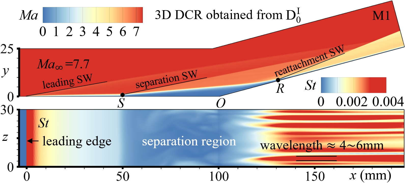
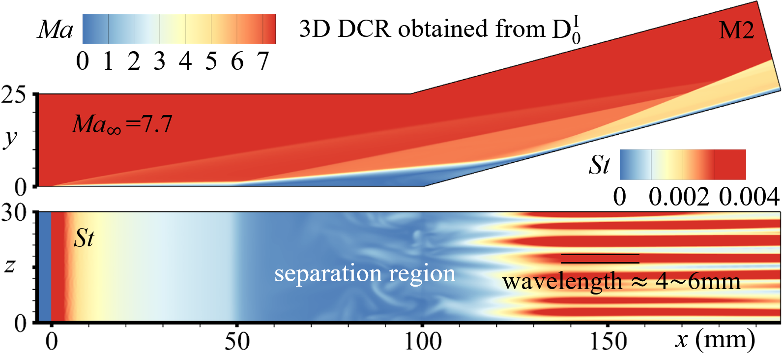
The 3D instantaneous flow fields of M1 and M2 are shown in Fig. 4. In the central planes, it clearly shows that the SW configurations include the leading edge SW, the separation SW, and the reattachment SW. In the first planes (on the wall), it can be noted that the wavelengths of the spanwise streaks on the ramp, colored by the Stanton number defined in Eq. 5, are about mm, which are consistent with the previous experimental observations (Roghelia et al., 2017a, b; Chuvakhov et al., 2017) and numerical results (Cao et al., 2021).
The aerothermodynamic characteristics are used to verify and validate the DNSs’ results, including the skin friction coefficient , the surface pressure coefficient , and the Stanton number , which are defined as
| (5) |
where , and are the friction, pressure and heat flux on the wall, respectively. and are the specific heat capacity and the adiabatic wall temperature, respectively.
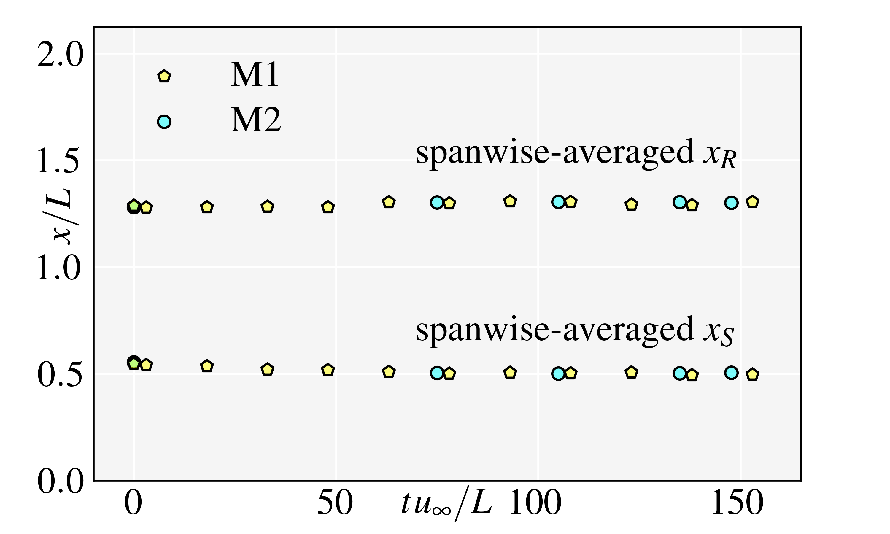
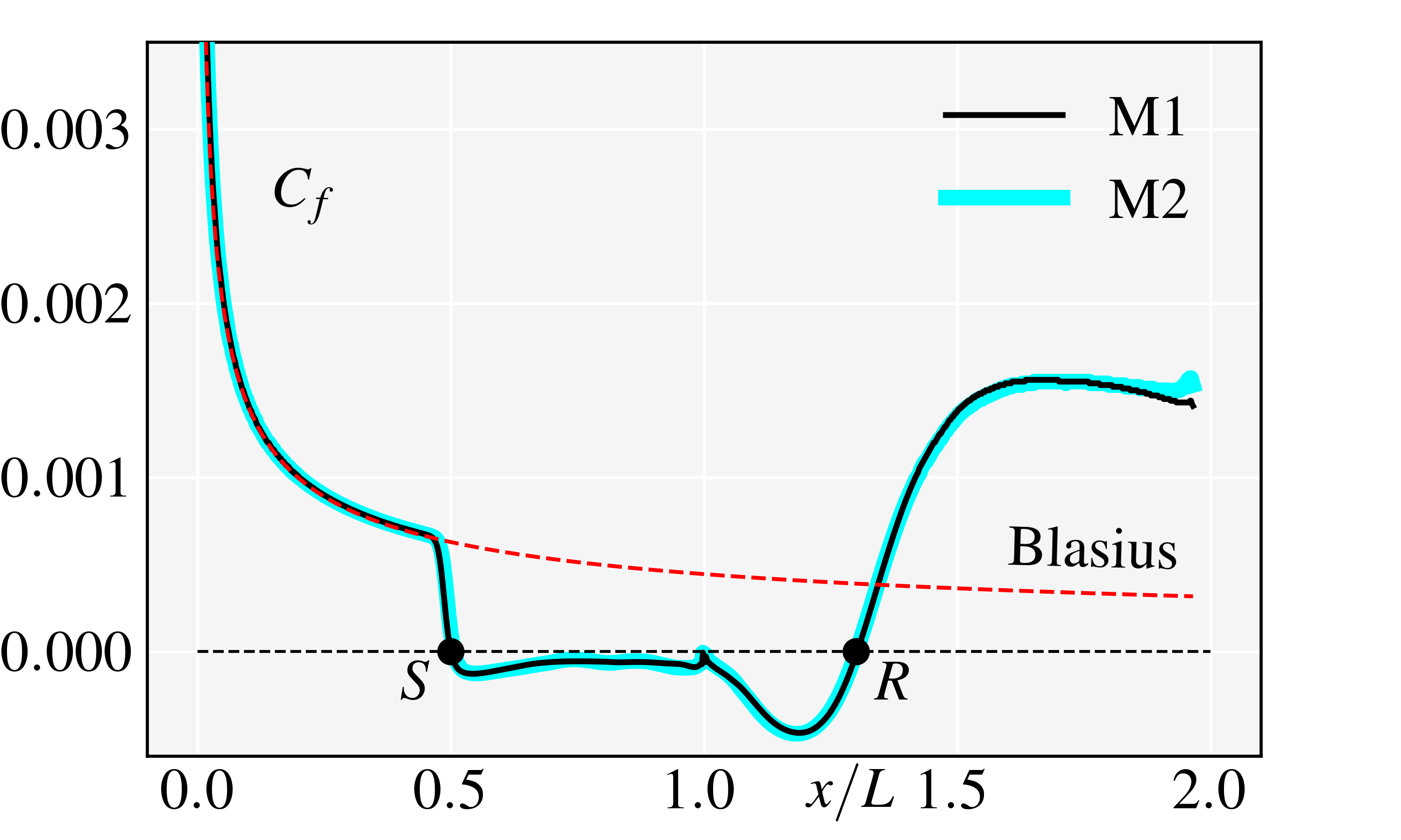
The verifications include the time- and grid-convergences. For the time-convergences, as shown in Fig. 5(a), the non-dimensional simulation time of M1 and M2 are both longer than . It shows that the spanwise-averaged locations of the separation and reattachment points only oscillate slightly near and after , implying the separated DCR flows have been stabilized in both M1 and M2. For the grid-convergence, as shown in Fig. 5(b), there are only small discrepancy of the distributions between M1 and M2, implying the mesh resolution of M1 is suitable for the present simulations.
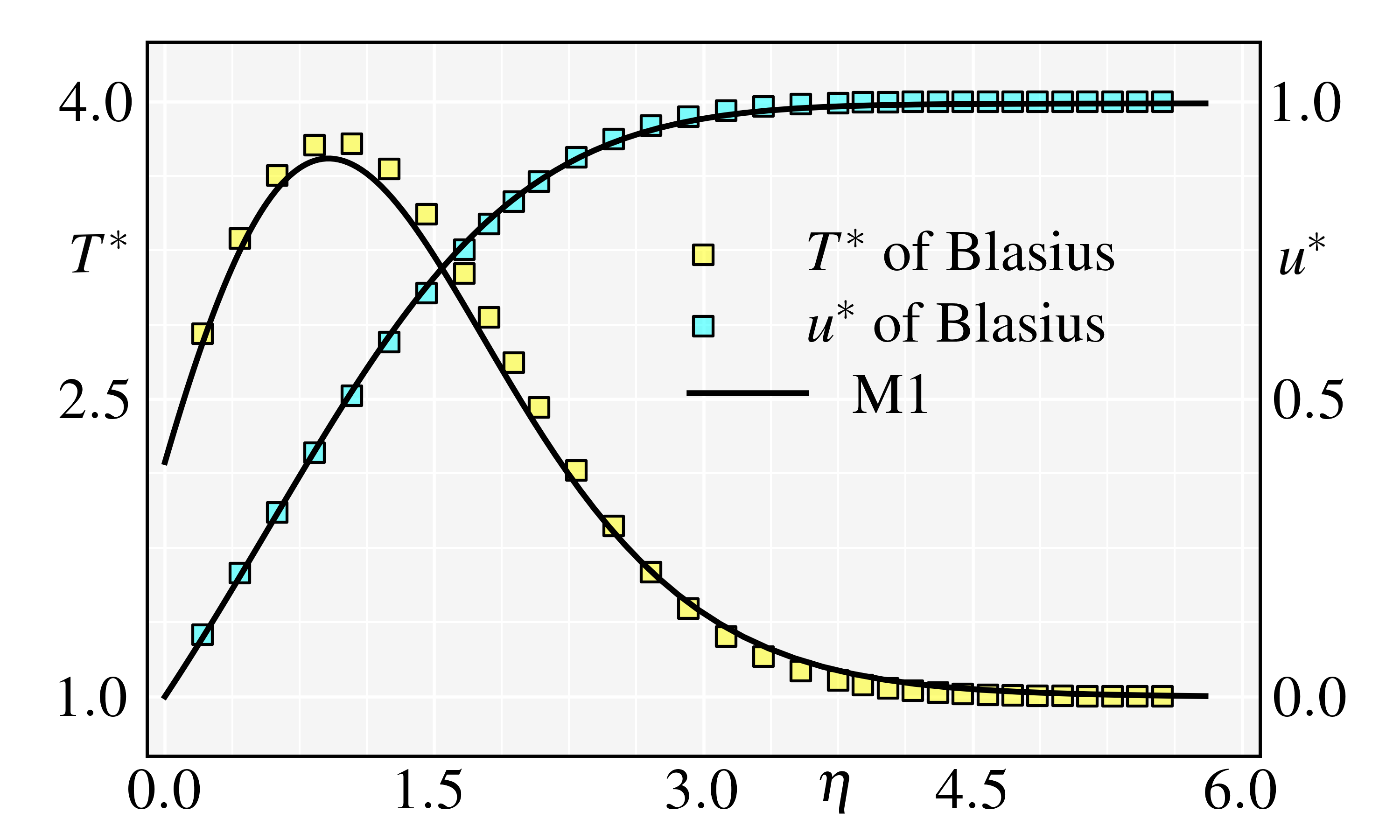
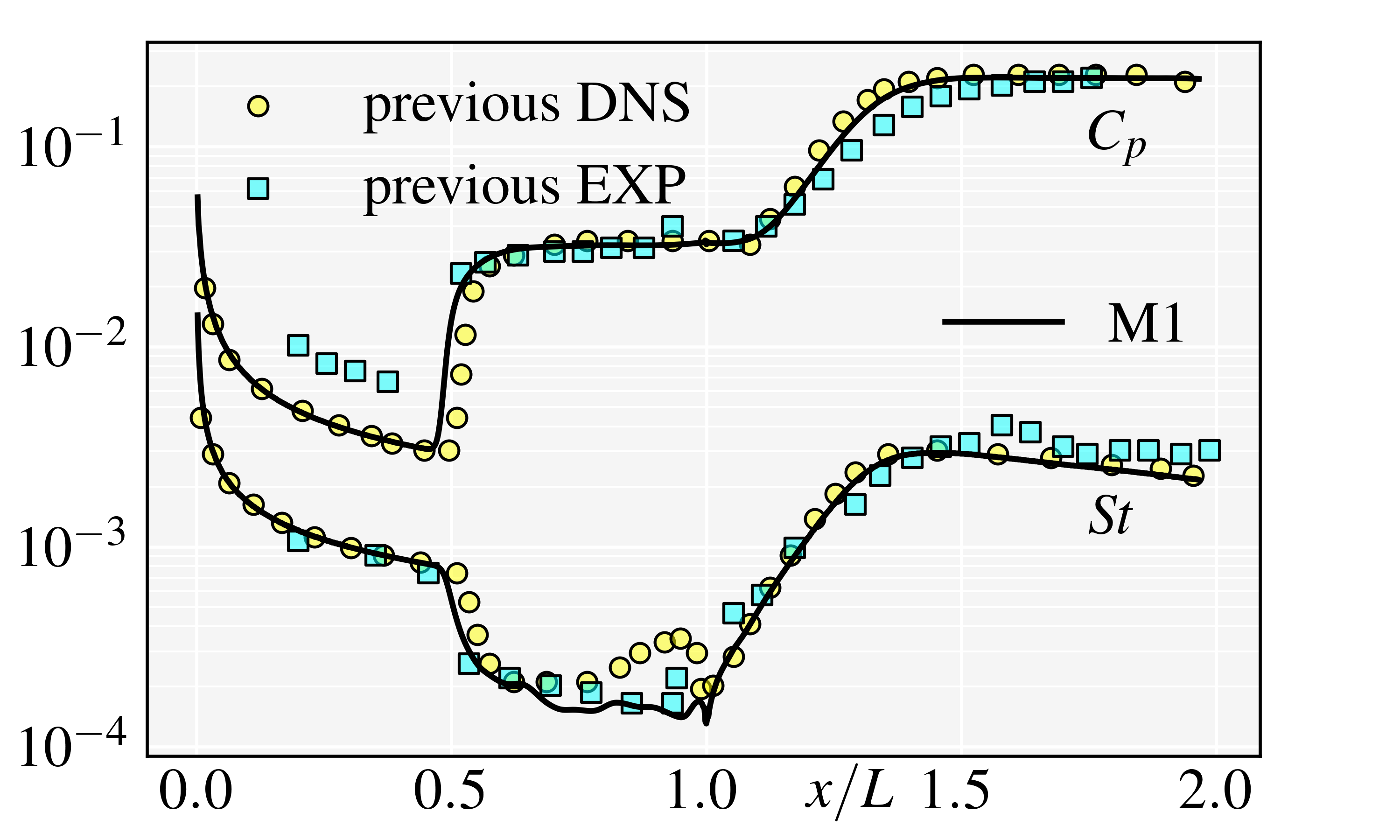
The validations include the comparisons of the present , , distributions, and , profiles with the accepted theoretical, numerical and experimental results. The laminar boundary layer before separation is self-similar satisfying the Blasius theoretical solutions (White & Majdalani, 2006). Fig. 5(b) shows the theoretical distribution, and Fig. 5(c) shows the theoretical normal profiles of and at . It is noted that both the present distribution and normal profiles agree well with the theoretical solutions, validating the simulations’ accuracy. Furthermore, as shown in Fig. 5(d), the present and distributions are also compared with the previous experiment (Roghelia et al., 2017a; Chuvakhov et al., 2017) and DNS (Cao et al., 2021) results, and the excellent agreements validate the present DNSs.
3.2 DNSs for bistable states of CCR flows
3.2.1 Numerical strategy to realize the thought experiment
As mentioned in Sec. 2, “adding the viscosity” and “filling the corner” are the key operations to realize the thought experiment. In terms of “adding the viscosity”, the implement method is changing the governing equations from Euler to Navier-Stokes. In terms of “filling the corner”, since it requires to fill the corner macroscopical continuously (fill the corner atom by atom, microscopically), the strict operation is to manipulate the flow fields with an enormous number of steps, the number of which is the order of magnitude of the Avogadro number. Obviously, it is impossible in numerical simulation, and the equivalent implement is to replace the filling mode from ‘macroscopically continuous’ to ‘macroscopically discrete’. The specific strategy is as follows.
For Route I (“adding the viscosity” “filling the corner”), the simulation process can be denoted as D C C … C, where the superscript ‘I’ denotes Route I, and the subscript ‘N’ represents the discrete number. Thus, D is the stable separated DCR flow in step 2, and C is the stable CCR flow after ‘N’ times of corner filling in step 3.
For Route II (“filling the corner” “adding the viscosity”), the simulation process is denoted as C C ,where C is the inviscid CCR flow in step 2, and C is the stale viscous flow in step 3, with the expectation of maintaining attached.
3.2.2 Simulations of Route I
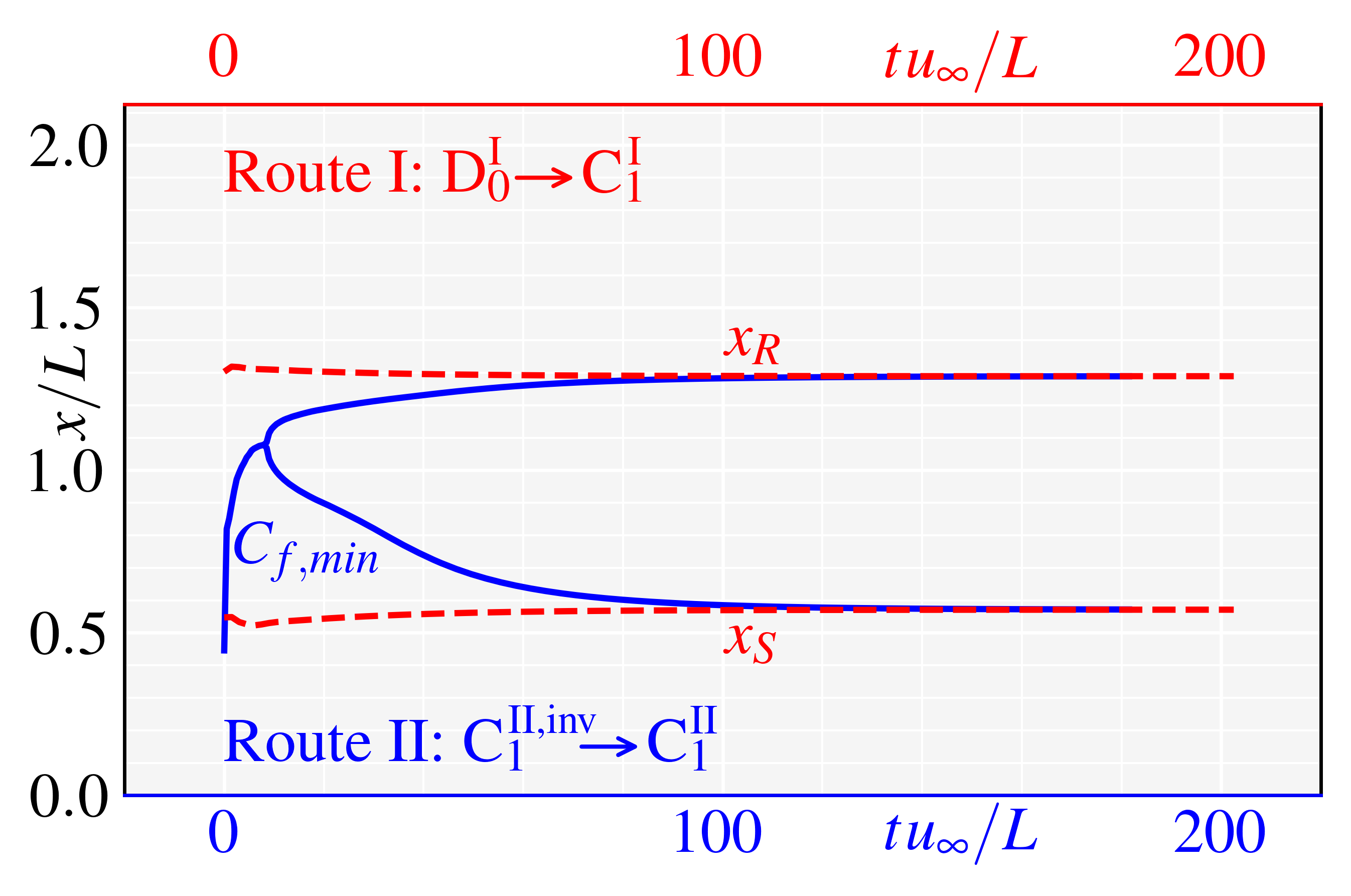
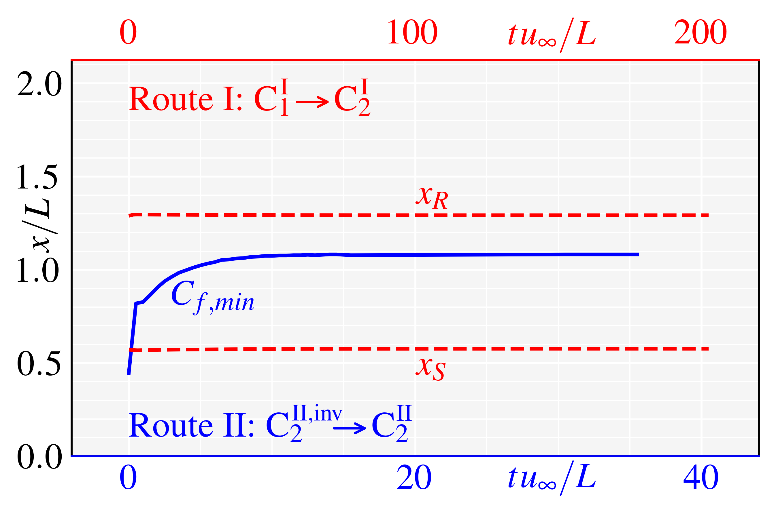
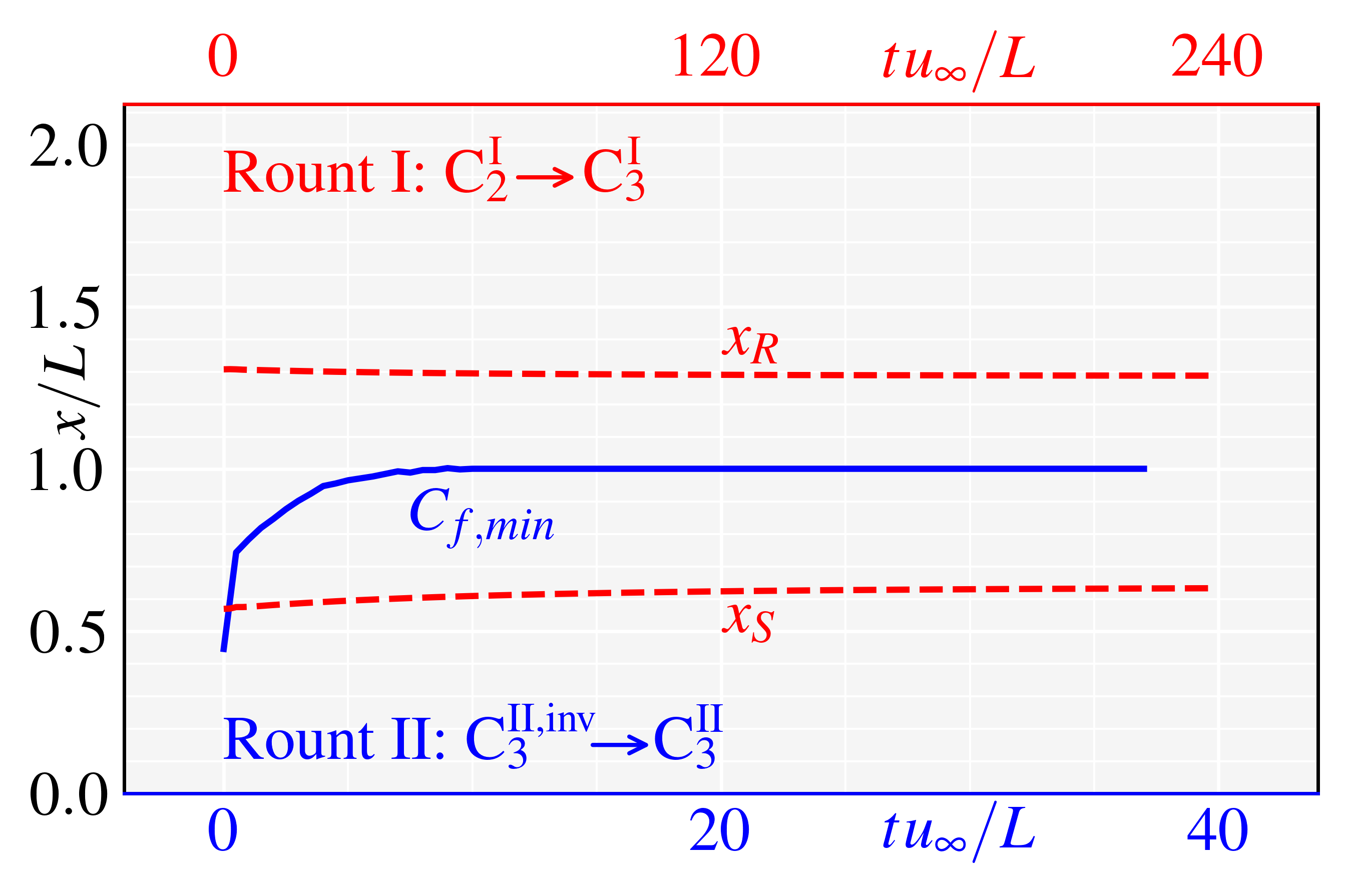
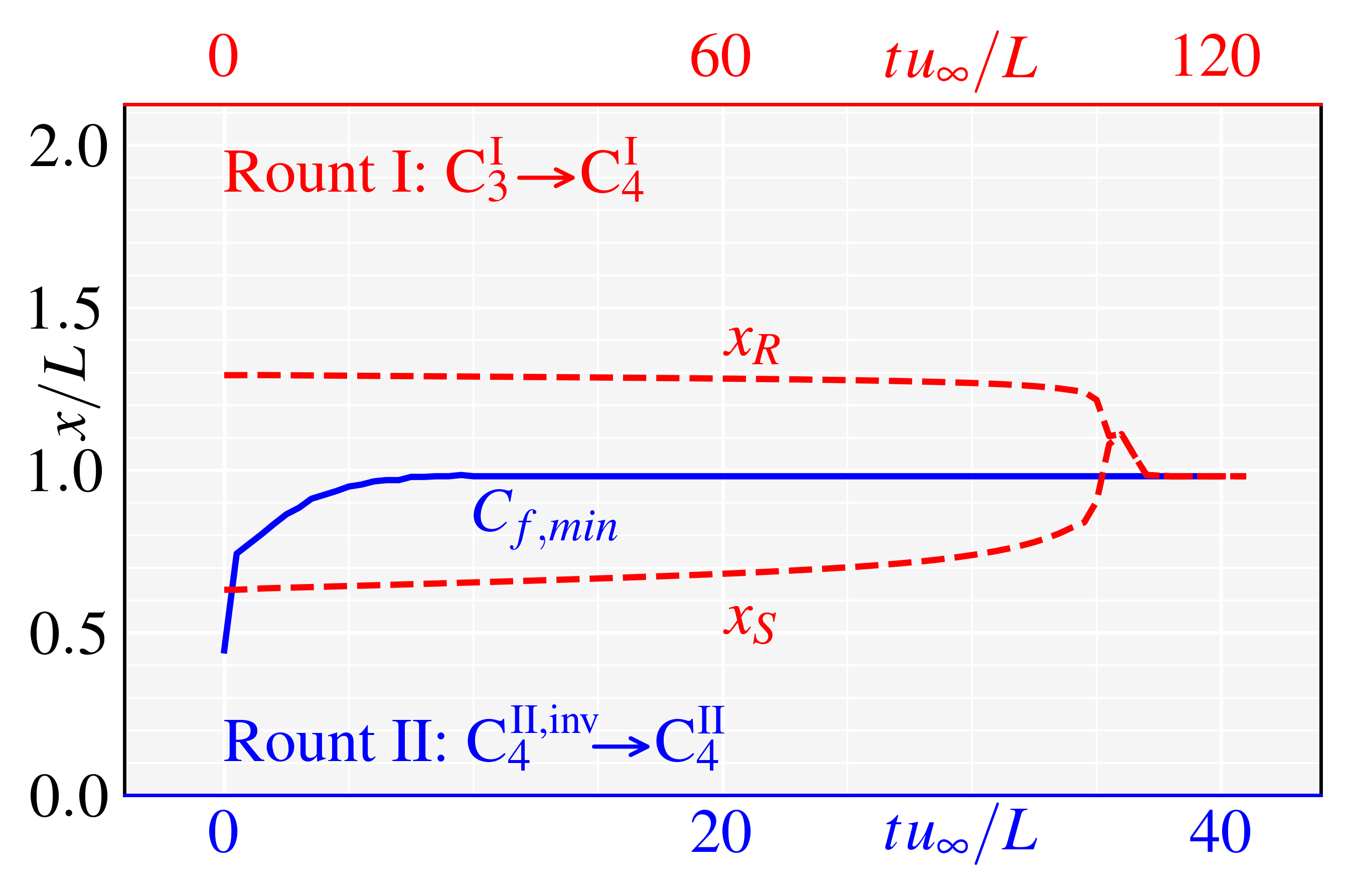
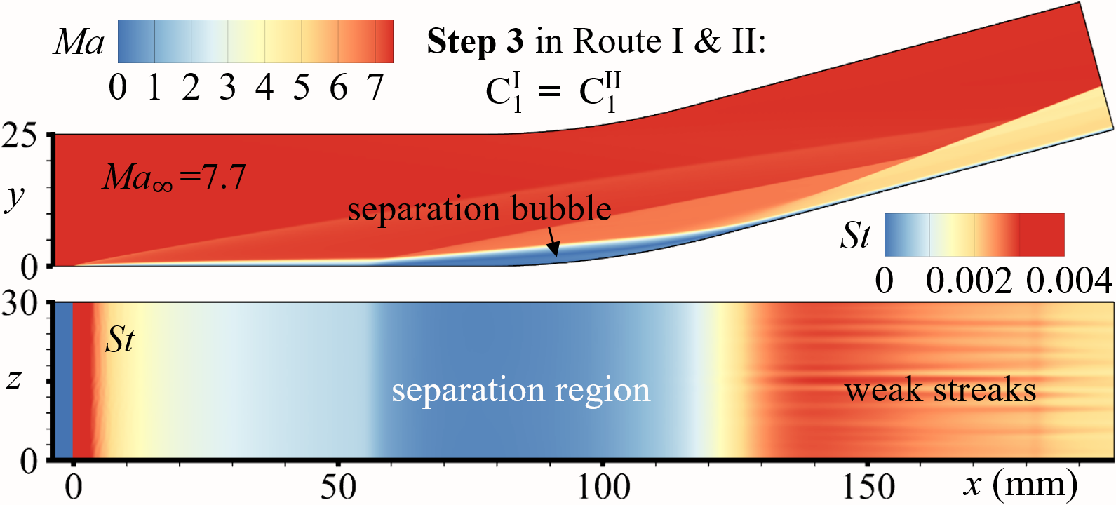
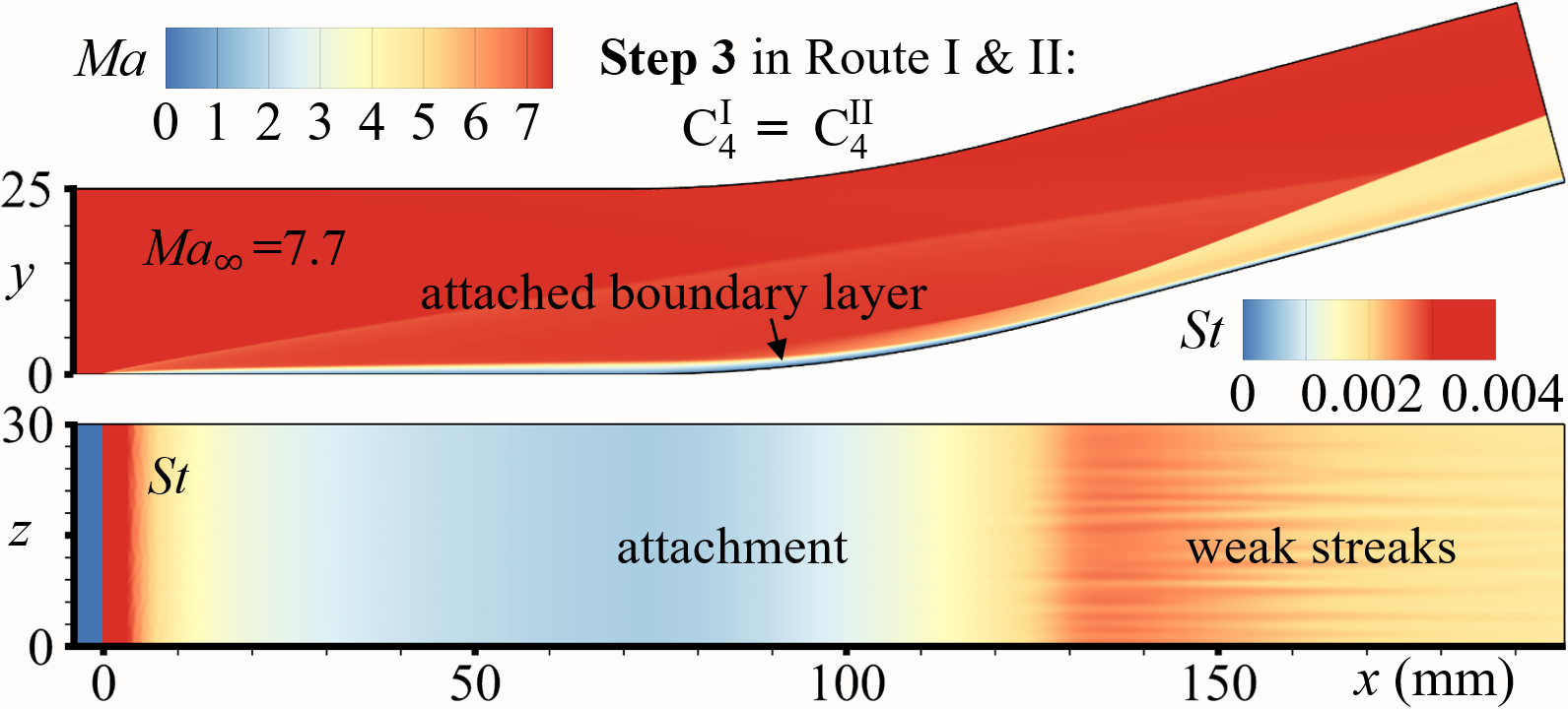
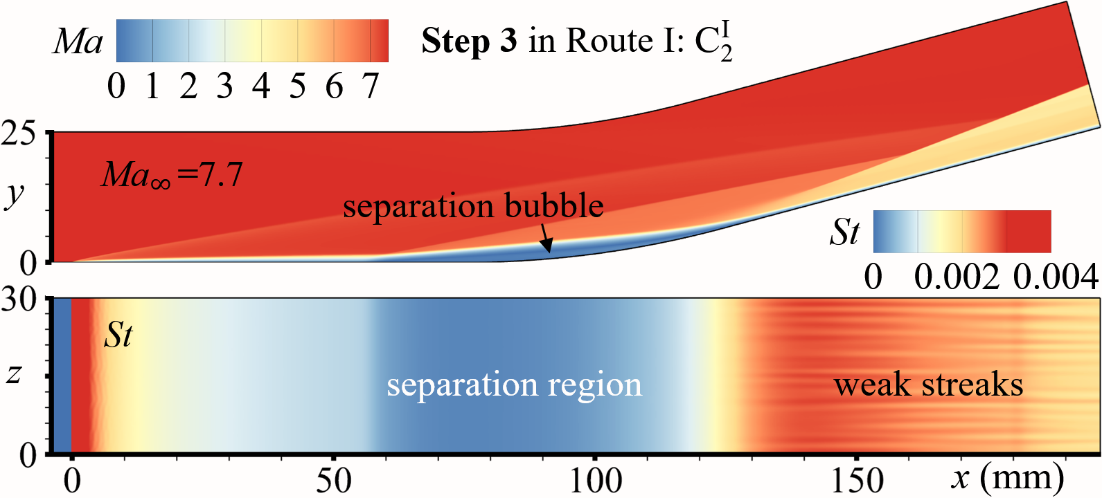
For D C C … C (Route I), we set N 4, and C1, C2, C3, C4 are four CCR configurations with curvature radiuses mm (mm), respectively. The four configurations’ meshes are set with the same resolution of M1 (). Three characteristic locations, , , and , are considered to quantify the flow states variations, where denotes the locations of minimal values in attached states. During process D C C C C, the evolutionary histories of spanwise-averaged and (red dashed lines) in C1, C1, C3, and C4 are shown in Fig.7(a), 7(b), 7(c), and 7(d), respectively, and the non-dimensional time (see the upper red -axes) for all cases. Obviously, and in C1, C2, and C3 are all maintaining two branches for , implying C, C, and C can all be stabilized at separated states. However, for C4 (the largest curvature radius), and ultimately merge into one branch (the branch— the blue solid line) at , implying C ends up in the attached state. Flow fields of C, C, C, and C are also shown in Fig. 9(a), 9(c), 9(e), and 9(b), respectively. It is noted that, on the ramp, the streaks in CCR are weaker than those in DCR.
3.2.3 Simulations of Route II
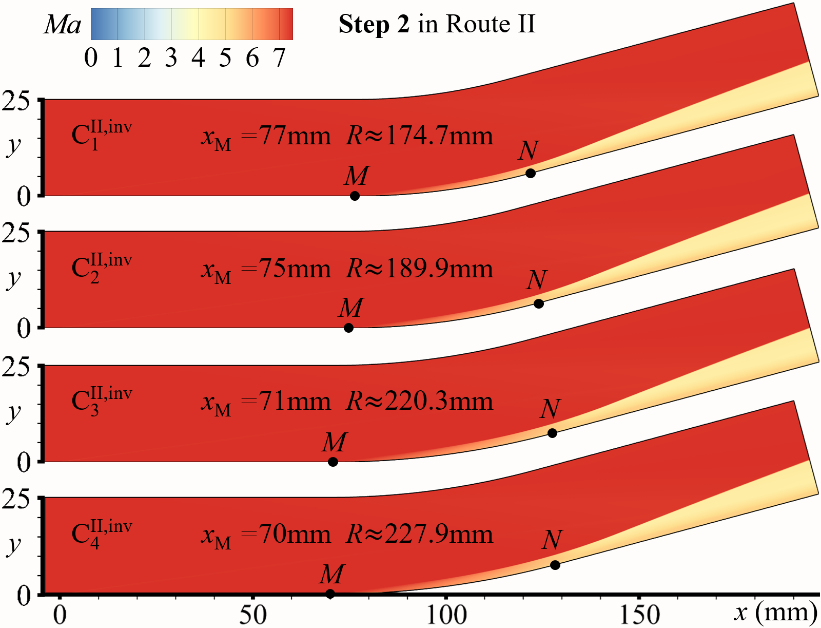
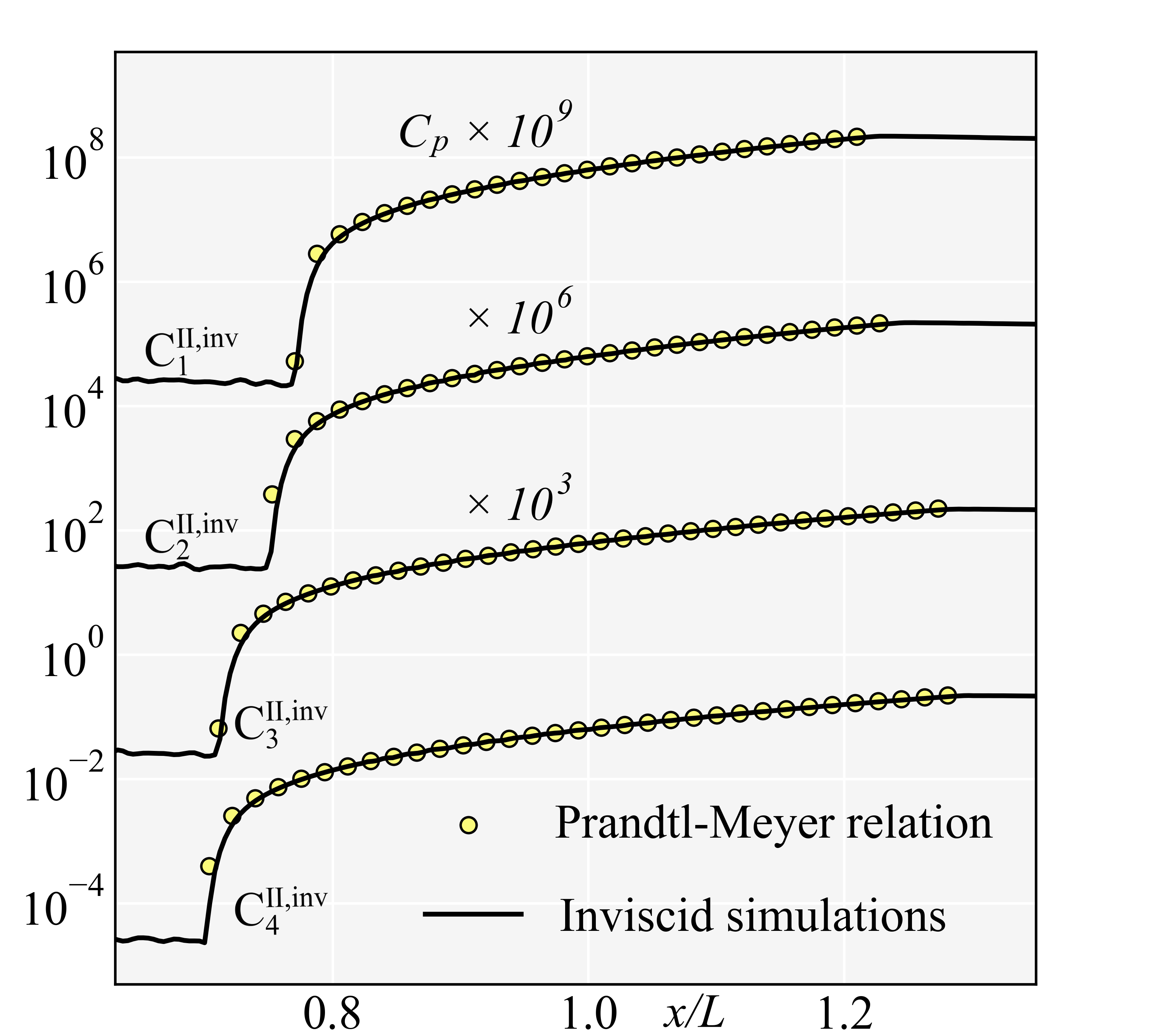
For C C (Route II), the flows in Step 2 (inviscid flows in C, N=4) are simulated with Euler equations, which are shown in Fig. 8(a) and denoted as C, C, C, and C, respectively. A series of compression waves distribute on the curved wall regions, and the distributions on satisfy the Prandtl-Meyer relations, as shown in Fig. 8(b), validating the present simulations.
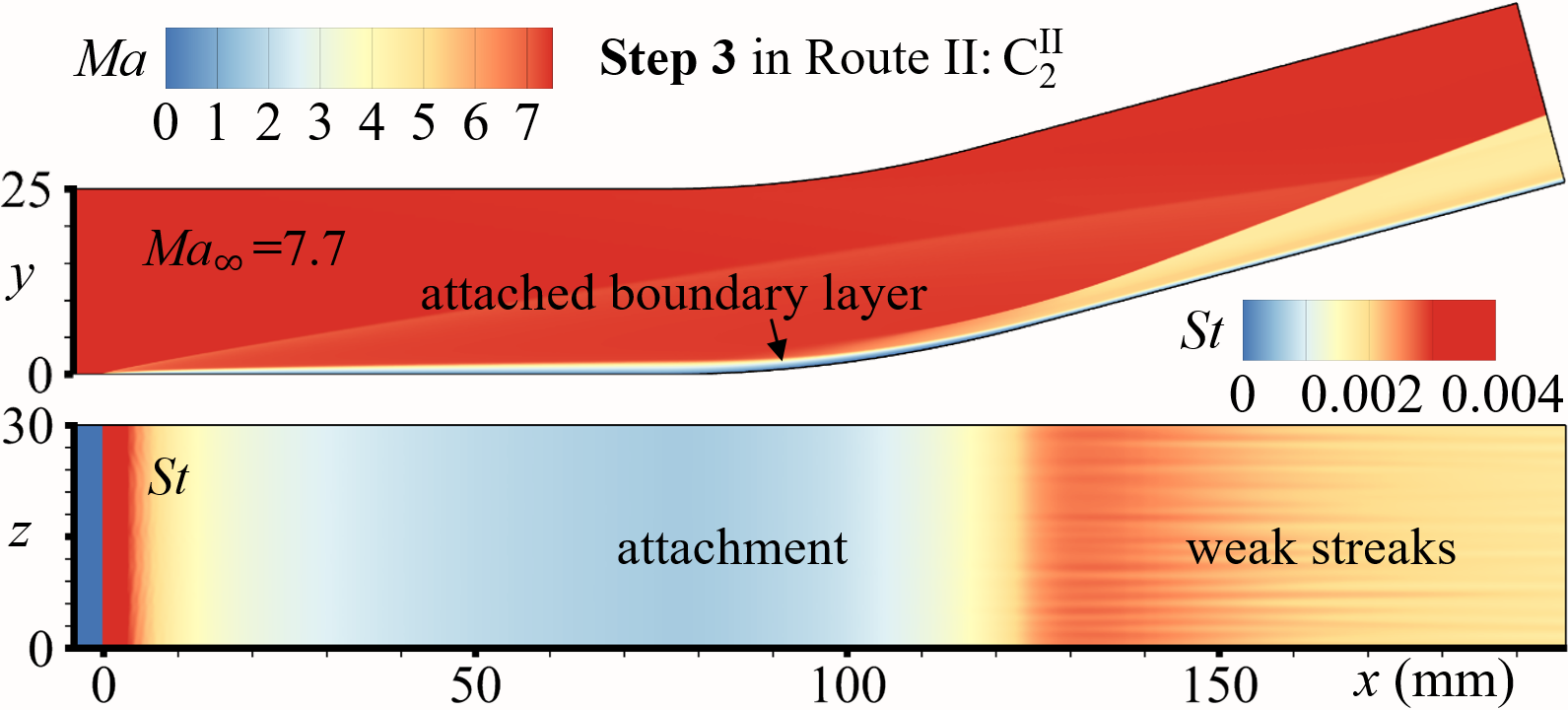
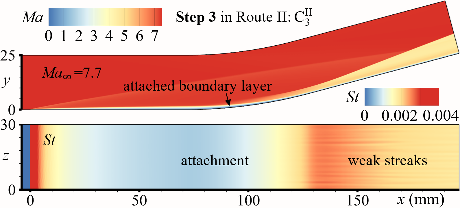
To accomplish Step 3 in Route II (adding viscosity), Euler equations are replaced with Navier-Stokes form, with the expectation of obtaining the stable attached states. The processes are denoted as C C, C C, C C, and C C, whose evolutionary histories of are respectively shown in Fig.7(a), 7(b), 7(c), and 7(d) (non-dimensional time for all cases, see the lower blue -axes). -variations in C2, C3, and C4 are similar: being of only one branch, first moving downstream and then stabilizing after about . This behavior implies C, C, and C all ultimately stabilize in attached states. However, in C (the smallest curvature radius), the bifurcates into two branches at . The lower and upper branches repectively converge to the and branches obtained from D C, implying C finally stabilizes in the separated state. Flow fields of C, C, C, and C are also shown in Fig. 9(a), 9(d), 9(f), and 9(b), respectively.

3.3 Contrast of the bistable states
The ultimate states of route I and II are listed in Table 2. For configuration C1, the ultimate states, C and C, are both separated as shown in Fig. 7(a); for configuration C4, the ultimate states, C and C, are both attached as shown in Fig. 7(c). It needs to be emphasized that, for configurations C2 and C3 (Fig. 7(b) and 7(c)), both separated states (C and C in Fig. 9(c) and 9(e)) and attached (C and C in Fig. 9(c) and 9(d)) states can be stably established for the same boundary conditions, verifying the existence of the bistable states in CCR flows. The ultimate states of route I and II are listed in Table 2. Also note that the weak streaks emerge in the downstream, implying the bistable states can resist disturbances of a certain intensity.
| C | C | C | C | C | C | C | C | |
|---|---|---|---|---|---|---|---|---|
| Separated | Separated | Separated | Attached | Separated | Attached | Attached | Attached |
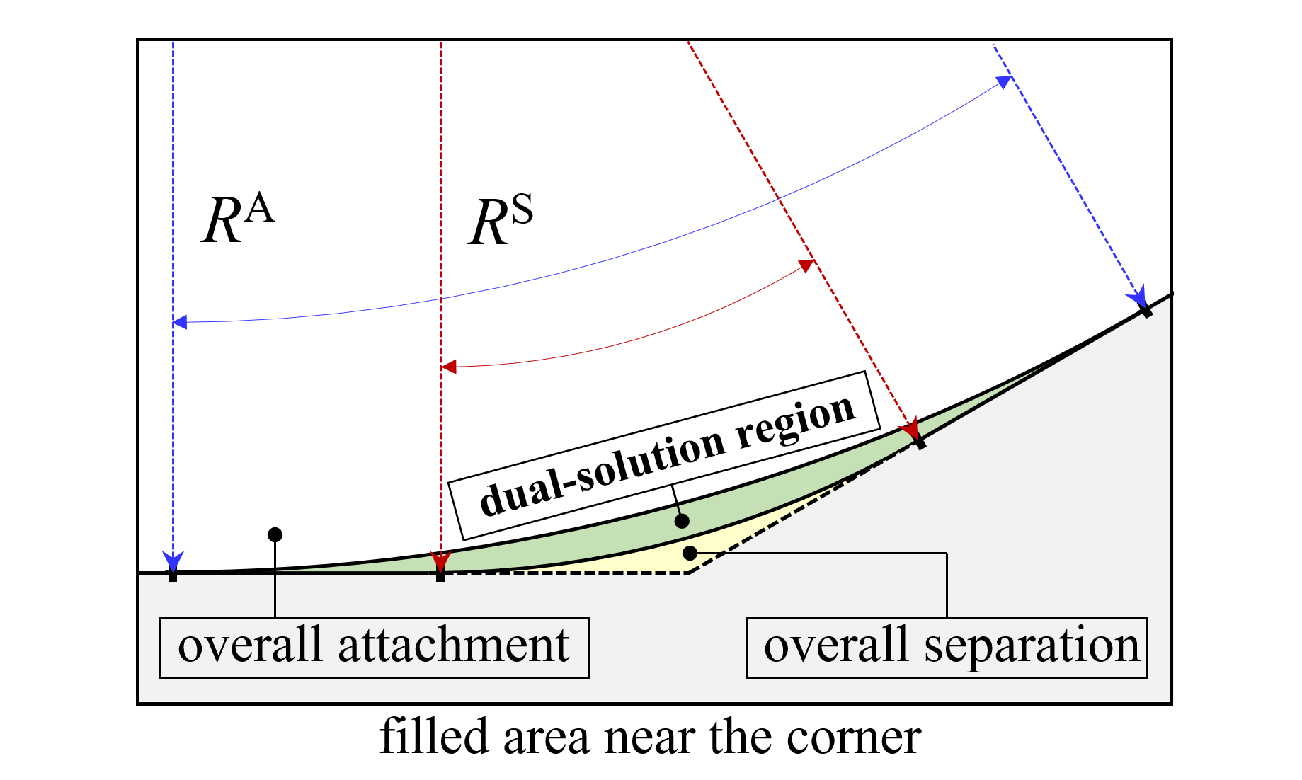
According to the ultimate states, the solution space of the flow field can be divided into three regions by two critical curvature radii, and , as shown in Fig. 10(a): only stable attached states exist when (the overall attachment region); only stable separated states exist when (the overall separation region— the yellow area ); both stable separate and attached states are physically possible when (the dual-solution region— the green area ). The filled-area ratio is used to characterize the relative proportions of the dual-solution region, which is defined as
| (6) |
In the present cases, with mm and mm. In other words, during the filling process, more than a quarter of the materials “break” the one-to-one corresponding relations from the configuration geometries to the flow states.
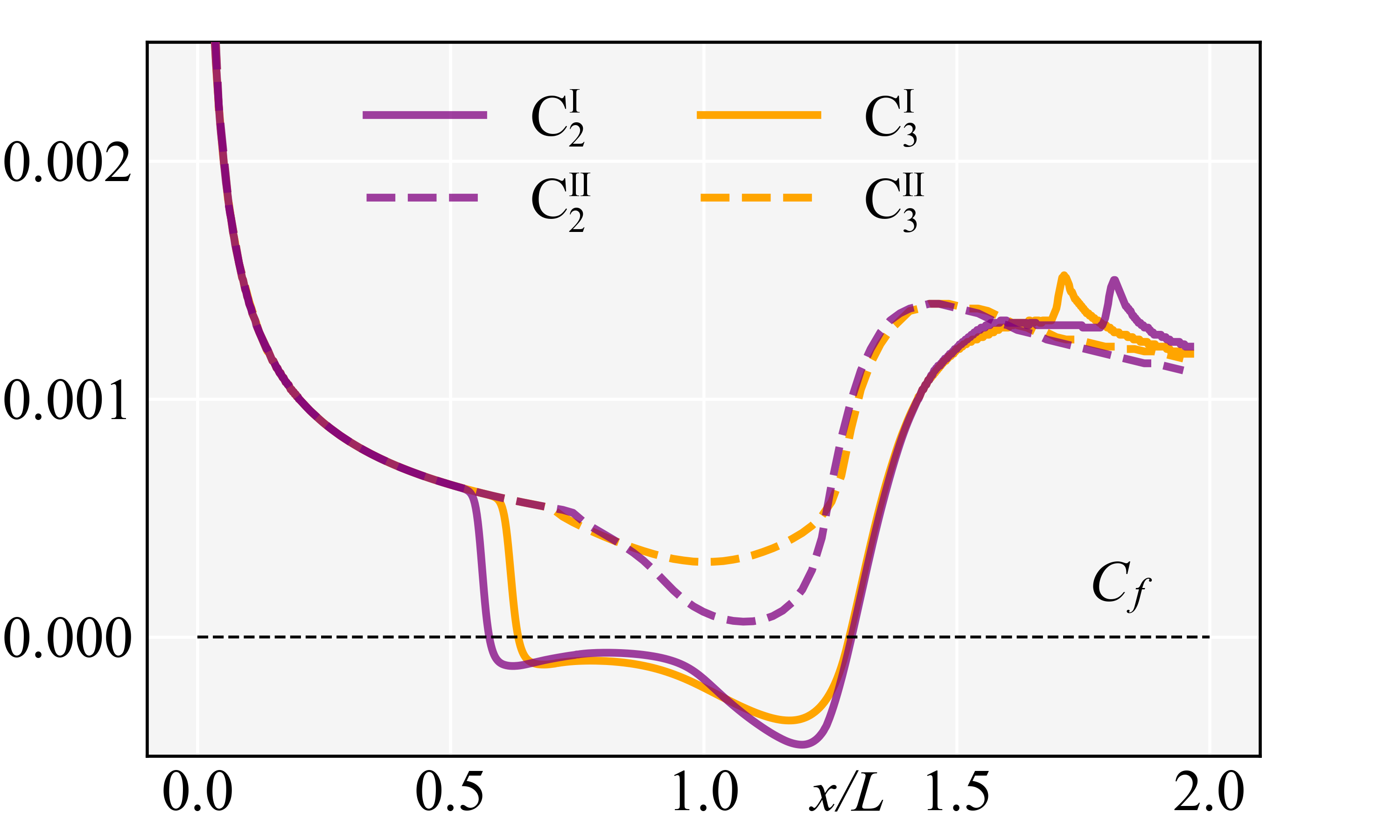
Furthermore, the aerothermodynamic characteristics including the distributions of spanwise-averaged , and on C2 and C3 are shown in Fig. 10. For both separated states (C and C) and attached (C and C) states of C2 and C3, all the distributions of collapse in the upstream part of the flat plate, so do and . However, in the downstream, the distributions are distinctly different. For the distributions, as shown in Fig. 10(b), C and C quickly drop to negatives after separation and sharply rise to positives after reattachment, and both of them have two minimal values in the seaparation regions; while both C and C stay positive, and have only one minimal value, severally. For distributions, as shown in Fig. 10(c), C and C present plateaus in the separation regions, rise sharply after reattachment and then reach peaks, severally; while both C and C continuously decrease till the starting points of the curved walls, and then rise in the form of isentropic compression. For the distributions, as shown in Fig. 10(d), C and C drop rapidly to near zero (O()) after separation, and then increase rapidly to the peaks; while C and C slowly decrease till the starting points , and then increase gradually. Additionally, in the downstream of the ramps, , , and of the separated states are all greater than those of the attached states.
4 Robustness study
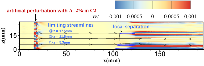
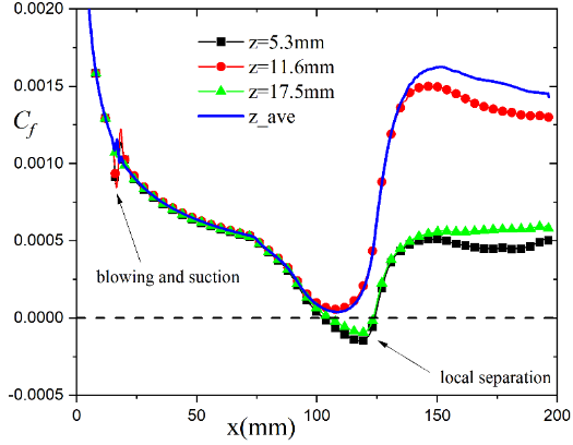
The phenomenon of bistability is somewhat counterintuitive, i.e., both separated and attached states can stably exist in C2 or C3 in the present cases, as shown in 2. To confirm its existence in the in the real physical world with disturbances, we further investigate the robustness of this phenomenon. Specifically, the attached states, C and C, are studied with some disturbances imparted to the upstream flow.
The disturbances have the following form, a region of steady blowing and suction, referring to Pirozzoli et al. (2004),
| (7) |
with the amplitude of the disturbance, the freestream velocity, and
| (8) | ||||
The locations mm and mm denote the beginning and the end of the disturbance region, respectively. Two amplitudes, and , are chosen to the investigate the influence of the disturbance strengths. mm is the spanwise width of the computational domain. is a random number ranging between 0 and 1. Three cases are considered, i.e., & for C and for C, all of which are simulated for , and the results shown below are all at .
For C (the smaller curvature radius Rmm), the weaker disturbance () can not perturb the attached state into a separated state, as shown in Fig. 11, while the stronger disturbance () make the downstream boundary locally separate at mm mm, as shown in Fig. 12. This implies that the stable attached state in C2 can at least resist a disturbance with the amplitude of , and for a fixed shape, the weaker the disturbance, the less likely the attached state is to be broken.
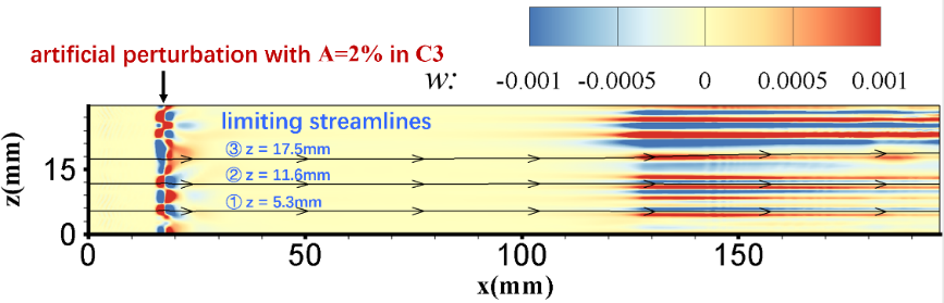
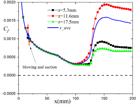
For C (the larger curvature radius Rmm), even the stronger disturbance () can not perturb the attached state into a separated state, as shown in Fig. 13. In fact, it can be seen that the on the curved wall in C3 is larger (a greater distance from ) than that of C2, which can resist a stronger disturbance. This implies that, for a certain disturbance, the larger the curvature radius, the more robust the attached state.
The above results imply that the bistable states can resist disturbances of a certain intensity; the larger the curvature radius, the more robust the attached state; the smaller the curvature radius, the more robust the separated state.
5 Conclusions
The CCR flows’ bistability is conjectured through a thought experiment and verified using the 3D DNSs. The dual-solution region in the present cases accounts for more than 25 percent of the total filling area. The differences of bistable aerothermodynamic are compared. As an intrinsic property, CCR’s bistability originates from the bifurcation characteristics of Navier-Stokes equations, and its specific presentation process can be diverse, corresponding to the hystereses induced by different parameter variations, such as , , and - variations, and some 2D cases have been reported (Hu et al., 2020; Zhou et al., 2021).
Next, we will design wind tunnel experiments to show the bistable states of CCR flows, which is more interesting and challenging. After all, it took more than 100 years from Mach’s discovery (Mach, 1878) of two SW reflection patterns to the observation of their bistable states in the wind tunnel (Chpoun & Ben-Dor, 1995). In some sense, there is systematic similarity between CCR flows and SW reflections: local subsonic regions (separation bubbles in CCR flows, and subsonic regions behind Mach stems in SW reflections) exist in the global supersonic/hypersonic flows, making the flow systems have both hyperbolic and elliptic characteristics. Therefore, the geometrical parameters, curvature radius and wedge angle , play the similar role in the bistabilities of CCR flows and SW reflections, respectively.
SBLIs, represented by CCR flows, and Shock-Shock interactions (SSIs), represented by SW reflections (Ben-Dor et al., 2001), often dominate the complex flow in supersonic/hypersonic flight together. Therefore, more complex multistable shock patterns will be formed when multistable states of SBLIs and SSIs interact with each other, and the resultant complex aerothermodynamic characteristics need to be paid more attention in the future.
Acknowledgment
This work is supported by the National Key R & D Program of China (Grant No.2019YFA0405300). We look forward to receiving helpful comments from reviewers.
Declaration of interests. The authors report no conflict of interest.
References
- Babinsky & Harvey (2011) Babinsky, H. & Harvey, J. K. 2011 Shock Wave-Boundary-Layer Interactions.
- Ben-Dor et al. (2001) Ben-Dor, G., Vasiliev EI., Elperin, T. & Chpoun, A. 2001 Hysteresis phenomena in the interaction process of conical shock waves: experimental and numerical investigations. J. Fluid Mech. 448.
- Cao et al. (2021) Cao, S. B., Hao, J., Klioutchnikov, I., Olivier, H. & Wen, C. Y. 2021 Unsteady effects in a hypersonic compression ramp flow with laminar separation. J. Fluid Mech. 912.
- Chapman et al. (1958) Chapman, D. R., Kuehn, D. M. & Larson, H. K. 1958 Investigation of separated flows in supersonic and subsonic streams with emphasis on the effect of transition .
- Chpoun & Ben-Dor (1995) Chpoun, A., Passerel D. Li H. & Ben-Dor, G. 1995 Reconsideration of oblique shock wave reflections in steady flows. part 1. experimental investigation. J. Fluid Mech. 301, 19–35.
- Chuvakhov et al. (2017) Chuvakhov, P. V., Borovoy, V. Ya., Egorov, I. V., Radchenko, V. N., Olivier, H. & Roghelia, A. 2017 Effect of small bluntness on formation of görtler vortices in a supersonic compression corner flow. J. Appl. Mech. Tech. Phys. 58 (6), 975–989.
- Edney (1968) Edney, B. 1968 Anomalous heat transfer and pressure distributions on blunt bodies at hypersonic speeds in the presence of an impinging shock .
- Fu et al. (2021) Fu, L., Karp, M., Bose, S. T., Moin, P. & Urzay, J. 2021 Shock-induced heating and transition to turbulence in a hypersonic boundary layer. J. Fluid Mech. 909.
- Gai & Khraibut (2019) Gai, S. L. & Khraibut, A. 2019 Hypersonic compression corner flow with large separated regions. J. Fluid Mech. 877, 471–494.
- Ganapathisubramani et al. (2009) Ganapathisubramani, B., Clemens, N. T. & Dolling, D. S. 2009 Low-frequency dynamics of shock-induced separation in a compression ramp interaction. J. Fluid Mech. 636, 397–425.
- Gumand (1959) Gumand, W. J. 1959 On the plateau and peak pressure of regions of pure laminar and fully turbulent separation in two-dimensional supersonic flow. J. Aerosp. Sci. 26 (1), 56–56.
- Helm et al. (2021) Helm, C. M., Martín, M. P. & Williams, O. J.H. 2021 Characterization of the shear layer in separated shock/turbulent boundary layer interactions. J. Fluid Mech. 912.
- Hu et al. (2017) Hu, Y. C., Bi, W. T., Li, S. Y. & She, Z. S. 2017 beta-distribution for reynolds stress and turbulent heat flux in relaxation turbulent boundary layer of compression ramp. Sci. China: Phys., Mech. Astron. 60 (12), 124711.
- Hu et al. (2020) Hu, Y. C., Zhou, W. F., Wang, G., Yang, Y. G. & Tang, Z. G. 2020 Bistable states and separation hysteresis in curved compression ramp flows. Phys. Fluids 32 (11), 113601.
- Hung (1973) Hung, F. T. 1973 Interference heating due to shock wave impingement on laminar boundary layers. In 6th Fluid and PlasmaDynamics Conference.
- Jiang & Shu (1996) Jiang, Guang-Shan & Shu, Chi-Wang 1996 Efficient implementation of weighted eno schemes. Journal of computational physics 126 (1), 202–228.
- Mach (1878) Mach, E. 1878 Uber den verlauf von funkenwellen in der ebene und im raume. Sitzungsbr. Akad. Wiss. Wien 78, 819–838.
- Neiland (1969) Neiland, V. Y. 1969 Theory of laminar boundary layer separation in supersonic flow. Fluid Dyn. 4 (4).
- Pirozzoli et al. (2004) Pirozzoli, Sergio, Grasso, F & Gatski, TB 2004 Direct numerical simulation and analysis of a spatially evolving supersonic turbulent boundary layer at m= 2.25. Physics of fluids 16 (3), 530–545.
- Roghelia et al. (2017a) Roghelia, A., Chuvakhov, P. V., Olivier, H. & Egorov, I. 2017a Experimental investigation of görtler vortices in hypersonic ramp flows behind sharp and blunt leading edges. AIAA paper p. 3463.
- Roghelia et al. (2017b) Roghelia, A., Olivier, H., Egorov, I. V. & Chuvakhov, P. V. 2017b Experimental investigation of görtler vortices in hypersonic ramp flows. Exp. Fluids 58, 1–15.
- Simeonides & Haase (1995) Simeonides, G. & Haase, W. 1995 Experimental and computational investigations of hypersonic flow about compression ramps. J. Fluid Mech. 283 (-1), 17–42.
- Stewartson & Williams (1969) Stewartson, K. & Williams, P. G. 1969 Self-induced separation. Proc. R. Soc. London, Ser. A 312 (1509).
- Tang et al. (2021) Tang, M. Z., Wang, G., Hu, Y. C., Zhou, W. F., Xie, Z. X. & Yang, Y. G. 2021 Aerothermodynamic characteristics of hypersonic curved compression ramp flows with bistable states. Phys. Fluids 33 (12), 126106.
- Tao et al. (2014) Tao, Y., Fan, X. Q. & Zhao, Y. L. 2014 Viscous effects of shock reflection hysteresis in steady supersonic flows. J. Fluid Mech. 759, 134–148.
- Tong et al. (2017) Tong, F. L., Li, X. L., Duan, Y.H. & Yu, C. P. 2017 Direct numerical simulation of supersonic turbulent boundary layer subjected to a curved compression ramp. Phys. Fluids 29 (12), 125101.
- Wang et al. (2019) Wang, Q. C., Wang, Z. G., Sun, M. B., R.Yang, Zhao, Y.X. & Hu, Z. W. 2019 The amplification of large-scale motion in a supersonic concave turbulent boundary layer and its impact on the mean and statistical properties. J. Fluid Mech. 863, 454–493.
- White & Majdalani (2006) White, F.M. & Majdalani, J. 2006 Viscous fluid flow, , vol. 3. McGraw-Hill New York.
- Xu et al. (2021) Xu, D. H., Wang, J. C., Wan, M. P., Yu, C. P., Li, X. L. & Chen, S. Y. 2021 Effect of wall temperature on the kinetic energy transfer in a hypersonic turbulent boundary layer. J. Fluid Mech. 929.
- Zhou et al. (2021) Zhou, W. F., Hu, Y. C., Tang, M. Z., Wang, G., Fang, M. & Yang, Y. G. 2021 Mechanism of separation hysteresis in curved compression ramp. Phys. Fluids 33 (10), 106108.