The bifurcation structure within robust chaos for two-dimensional piecewise-linear maps.

Complex dynamics are caused by nonlinearity, and many physical systems involve an extreme form of nonlinearity: a switch. Examples include engineering systems with relay or on/off control which involve distinct modes of operation [5, 23, 43]. Mathematical models of systems with switches are naturally piecewise-smooth, where different pieces of the equations correspond to different positions of a switch.

Piecewise-smooth maps arise as discrete-time models of systems with switches [16, 33] and as Poincaré maps or stroboscopic maps of continuous-time models [7]. For multi-dimensional piecewise-smooth maps there are many abstract ergodic theory results stating that if an attractor satisfies certain properties (e.g. expansion) then it is chaotic in a certain sense (e.g. has an SRB measure) [6, 30, 35, 42, 45]. This paper in contrast provides explicit results for a physically-motivated family of maps. We study the four-parameter family

$\displaystyle f_{\xi}(x,y)=\begin{cases}\begin{bmatrix}\tau_{L}x+y+1\\ -\delta_{L}x\end{bmatrix},&x\leq 0,\\ \begin{bmatrix}\tau_{R}x+y+1\\ -\delta_{R}x\end{bmatrix},&x\geq 0,\end{cases}$

(1.1)

where $\xi=(\tau_{L},\delta_{L},\tau_{R},\delta_{R})\in\mathbb{R}^{4}$. This is known as the two-dimensional border-collision normal form (BCNF) [26]. This family provides leading-order approximations to border-collision bifurcations where a fixed point of a piecewise-smooth map collides with a switching manifold as parameters are varied [36]. As such (1.1) can be used to capture the change in dynamics as parameters are varied to pass through border-collision bifurcations. In this regards it has been applied to mechanical oscillators with stick-slip friction [41], DC/DC power converters [47], and various models in economics [33]. We stress that unlike Poincaré maps of smooth invertible flows, the piecewise-smooth maps arising from these applications are mostly non-invertible. We distinguish four generic cases based on the signs of the determinants $\delta_{L}$ and $\delta_{R}$:

• •

  With $\delta_{L}>0$ and $\delta_{R}>0$ (1.1) is orientation-preserving. This is the classical scenario considered in the ‘robust chaos’ paper of Banerjee et al [4].

• •

  With $\delta_{L}<0$ and $\delta_{R}<0$ (1.1) is orientation-reversing. Misiurewicz [25] used this scenario in the subfamily of Lozi maps ($\tau_{L}=-\tau_{R}$, $\delta_{L}=\delta_{R}$) for his novel rigorous demonstration of robust chaos.

• •

  With $\delta_{L}>0$ and $\delta_{R}<0$ (1.1) is non-invertible mapping both the left half-plane ($x\leq 0$) and the right half-plane ($x\geq 0$) onto the upper half-plane ($y\geq 0$). This scenario applies to border-collision bifurcations in a wide range of power converters whereby a switch in a circuit creates non-invertible dynamics [3, 8, 46].

• •

  With $\delta_{L}<0$ and $\delta_{R}>0$ (1.1) is again non-invertible with applications to power electronics, but now maps to the lower half-plane ($y\leq 0$) and exhibits different dynamical features (notice (1.1) maps the origin to the right half-plane so does not have left/right symmetry).

Despite its apparent simplicity (1.1) has an incredibly complex bifurcation structure that remains to be fully understood [2, 10, 38, 40, 47]. The most significant bifurcations are those at which the attractor splits into pieces. In [12] we used renormalisation to uncover an infinite sequence of codimension-one bifurcations. However, this only accommodated the orientating-preserving setting of Banerjee et al [4]. In this paper we identify similar sequences of bifurcations in the orientation-reversing and non-invertible parameter regimes. Again we use renormalisation to find bifurcations, but now this approach misses some bifurcations. For this reason we combine the analytical framework with brute-force numerical simulations that compute the number of connected components from the behaviour of forward orbits.

The remainder of this paper is organised as follows. We start in §2 by reviewing the bifurcation structure of one-dimensional piecewise-linear maps (skew tent maps) and how this structure can be generated through renormalisation. This corresponds to the BCNF in the special case $\delta_{L}=\delta_{R}=0$, and it is helpful to view the bifurcation structures described in later sections as extensions or perturbations from the structure that arises in one dimension. Then in §3 we review the parameter region $\Phi\subset\mathbb{R}^{4}$ where the BCNF has two saddle fixed points. We describe special points on the stable and unstable manifolds of the fixed points whose relation to one another can be used to characterise the occurrence of homoclinic and heteroclinic bifurcations where the attractor is destroyed. In §4 we introduce the renormalisation scheme and describe some basic aspects of this scheme that hold for all values of $\delta_{L}$ and $\delta_{R}$. Then in §5 we summarise the results of [12] for the orientation-preserving setting.

Next in §6 we describe an algorithm for numerically determining the number of connected components of attractor. The algorithm outputs the greatest common divisor of a set of iteration numbers required for an orbit to return close to its starting point. The algorithm is effective when the components of attractor are not too close to one another and the dynamics on the attractor is ergodic. Applied to the orientation-preserving setting it reproduces the bifurcation structure obtained by renormalisation.

In §7, §8, and §9 we study the orientation-reversing and non-invertible cases and explain why the same renormalisation scheme should be expected to work in these settings. Formal proofs are beyond the scope of this study because, as evident from [12], these require a detailed analysis of the four-dimensional nonlinear renormalisation operator, plus will involve additional complexities because now stable period-two and period-four solutions are possible. Also if $\delta_{L}<0$ and $\delta_{R}>0$ then the bifurcations that destroy the attractor are different and more difficult to characterise. In §10 we describe a special case unique to the non-invertible settings where the dynamics reduces to one dimension. Concluding remarks are provided in §11.

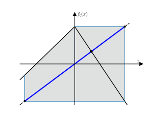
With $\delta_{L}=\delta_{R}=0$ the $y$-dynamics of (1.1) is trivial and the $x$-dynamics reduces to

$\displaystyle x\mapsto\begin{cases}\tau_{L}x+1,&x\leq 0,\\ \tau_{R}x+1,&x\geq 0.\end{cases}$

(2.1)

This is a two-parameter family of skew tent maps. For any values of the parameters $\tau_{L}$ and $\tau_{R}$ for which (2.1) has an attractor, this attractor is unique. Fig. 1 shows typical examples of the attractor using $\tau_{L}>1$ and $\tau_{R}<-1$ with which (2.1) is piecewise-expanding, so the attractor is chaotic in a strict sense by the results of Lasota and Yorke [21] and Li and Yorke [22]. Fig. 1 shows typical examples of the chaotic attractor. In panel (a) the attractor is the interval $[\tau_{R}+1,1]$ whose endpoints are the first and second iterates of the switching value $x=0$. In panel (b) the attractor is a disjoint union of four intervals whose endpoints are the first through eighth iterates of $x=0$.

For all values of $\tau_{L}$ and $\tau_{R}$ the nature of the attractor is well understood [24, 27, 39]. Fig. 2 shows how the part of the $(\tau_{L},\tau_{R})$-plane that is relevent to us divides into regions according to the number of intervals that comprise the attractor. In the top-left region labelled $LR$ the map has a stable period-two solution. This solution has one point in the left half-plane and one point in the right half-plane, so is termed an $LR$-cycle. This region is bounded by the curve $\alpha_{0}(\tau_{L},\tau_{R})=0$, where

$\displaystyle\alpha_{0}(\tau_{L},\tau_{R})=\tau_{L}\tau_{R}+1,$

(2.2)

which is where the $LR$-cycle loses stability by attaining a stability multiplier of $-1$. The boundary in the lower-right part of the figure is a homoclinic bifurcation where $x=0$ maps in two iterations to the fixed point of (2.1) in $x<0$. This occurs on the curve $\phi_{0}(\tau_{L},\tau_{R})=0$, where

$\displaystyle\phi_{0}(\tau_{L},\tau_{R})=\tau_{L}\tau_{R}+\tau_{L}-\tau_{R}.$

(2.3)

As shown by Ito et al [17, 18] the remaining boundaries can be identified through renormalisation as follows. Suppose there exists an interval neighbourhood $I$ of $x=0$ that maps into $x>0$, then, on the second iteration, back into $I$. In this case the restriction of the second iterate of (2.1) to $I$ is piecewise-linear with two pieces. The $x<0$ piece corresponds to iterates with symbolic itinerary $LR$ and has slope $\tau_{L}\tau_{R}<-1$, while the $x>0$ piece corresponds to iterates with symbolic itinerary $RR$ and has slope $\tau_{R}^{2}>1$. Thus the second iterate of (2.1) on $I$ is conjugate to (2.1) with $\tau_{R}^{2}$ in place of $\tau_{L}$ and $\tau_{L}\tau_{R}$ in place of $\tau_{R}$. This corresponds to the substitution rule $(L,R)\mapsto(RR,LR)$, and induces the renormalisation operator

$\displaystyle g(\tau_{L},\tau_{R})=(\tau_{R}^{2},\tau_{L}\tau_{R}).$

(2.4)

By using the preimages of the homoclinic bifurcation boundary we define the sequence of regions

$\displaystyle\mathcal{R}_{n}=\mathopen{}\mathclose{{}\left\{(\tau_{L},\tau_{R})\,\middle|\,\tau_{R}<-1,\phi_{0}\mathopen{}\mathclose{{}\left(g^{n}(\xi)}\right)>0,\phi_{0}\mathopen{}\mathclose{{}\left(g^{n+1}(\xi)}\right)\leq 0,\alpha_{0}(\tau_{L},\tau_{R})<0}\right\},$

(2.5)

shown in Fig. 2. These are non-empty for all $n\geq 0$ and converge to $(\tau_{L},\tau_{R})=(1,-1)$ as $n\to\infty$. In $\mathcal{R}_{0}$ the attractor consists of one interval:

A simple proof of Theorem 2.1 can be found in Veitch and Glendinning [44]. The condition $\tau_{L}\geq 1$ is needed because for some $0<\tau_{L}<1$ and $\tau_{R}<-1$ the attractor is periodic. This condition can be weakened but this is not needed for our purposes.

To characterise the attractor in the other regions $\mathcal{R}_{n}$ we first make the following observation that follows simply from the definitions of $g$ and $\mathcal{R}_{n}$.

Thus if $(\tau_{L},\tau_{R})\in\mathcal{R}_{n}$ then $g^{n}(\tau_{L},\tau_{R})\in\mathcal{R}_{0}$. Theorem 2.1 can be applied at this parameter point because any point below $\tau_{R}=-1$ maps under $g$ to the right of $\tau_{L}=1$. Moreover, the above conjugacy can be shown to hold under all $n$ applications of $g$, see Ito et al [17, 18], thus the $2^{n}$-iterate of (2.1) has an interval attractor. The images of this interval under (2.1) give $2^{n}$ disjoint intervals and hence the following result.

We now return to the BCNF (1.1) with non-zero values of $\delta_{L}$ and $\delta_{R}$. In this section we identify two saddle fixed points and compute some important points on their stable and unstable manifolds.

Motivated by Banerjee et al [4] we focus on the following subset of four-dimensional parameter space:

$\displaystyle\Phi=\mathopen{}\mathclose{{}\left\{\xi\in\mathbb{R}^{4}\ \middle|\ \tau_{L}>|\delta_{L}+1|,\tau_{R}<-|\delta_{R}+1|}\right\}.$

(3.1)

It is a simple exercise to show that $\Phi$ is the set of all parameter values for which (1.1) has two saddle fixed points [11]. These fixed points are

	$\displaystyle X$	$\displaystyle=\mathopen{}\mathclose{{}\left(\frac{-1}{\tau_{R}-\delta_{R}-1},\frac{\delta_{R}}{\tau_{R}-\delta_{R}-1}}\right),$		(3.2)
	$\displaystyle Y$	$\displaystyle=\mathopen{}\mathclose{{}\left(\frac{-1}{\tau_{L}-\delta_{L}-1},\frac{\delta_{L}}{\tau_{L}-\delta_{L}-1}}\right),$		(3.3)

where $X$ is in the open right half-plane $x>0$, and $Y$ is in the open left half-plane $x<0$. Let

$\displaystyle A_{L}$

$\displaystyle=\begin{bmatrix}\tau_{L}&1\\ -\delta_{L}&0\end{bmatrix},$

$\displaystyle A_{R}$

$\displaystyle=\begin{bmatrix}\tau_{R}&1\\ -\delta_{R}&0\end{bmatrix},$

(3.4)

denote the Jacobian matrices associated with $Y$ and $X$ respectively. With $\xi\in\Phi$ the matrix $A_{L}$ has eigenvalues $|\lambda_{L}^{s}|<1$ and $\lambda_{L}^{u}>1$, while $A_{R}$ has eigenvalues $|\lambda_{R}^{s}|<1$ and $\lambda_{R}^{u}<-1$.

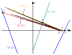
Since $X$ and $Y$ are saddles their stable and unstable manifolds are one-dimensional, and since the map is piecewise-linear these manifolds are piecewise-linear. Their stable manifolds $W^{s}(X)$ and $W^{s}(Y)$ have kinks on the switching manifold $x=0$ and at preimages of these points, while their unstable manifolds $W^{u}(X)$ and $W^{u}(Y)$ have kinks on the image of the switching manifold $y=0$ and at images of these points. For instance, as we grow $W^{u}(X)$ outwards from $X$, in one direction its first kink occurs at the point

$\displaystyle T=\mathopen{}\mathclose{{}\left(\frac{1}{1-\lambda_{R}^{s}},0}\right),$

(3.5)

on $y=0$, see Fig. 3. Similarly as we grow $W^{u}(Y)$ outwards from $Y$, in one direction its first kink occurs at

$\displaystyle D=\mathopen{}\mathclose{{}\left(\frac{1}{1-\lambda_{L}^{s}},0}\right).$

(3.6)

A third point $C$ will be also central to our later calculations. This point is where $W^{s}(Y)$, when grown outwards from $Y$ to the right, first intersects $y=0$ at a point with $x>0$ and is given by

$\displaystyle C=\mathopen{}\mathclose{{}\left(\frac{{\lambda_{L}^{u}}^{2}}{(\delta_{R}-\tau_{R}\lambda_{L}^{u})(\lambda_{L}^{u}-1)},0}\right).$

(3.7)

Fig. 3 indicates the points $T$, $D$, and $C$ for four example phase portraits, one for each of the four cases for the signs of $\delta_{L}$ and $\delta_{R}$. Notice if $\delta_{L}>0$ (upper plots) the left half-plane maps to the upper half-plane, while if $\delta_{L}<0$ (lower plots) the left half-plane maps to the lower half-plane. Similarly if $\delta_{R}>0$ (left plots) the right half-plane maps to the lower half-plane, while if $\delta_{R}<0$ (right plots) the right half-plane maps to the upper half-plane.

In §2 we saw that renormalisation based on the substitution rule $(L,R)\mapsto(RR,LR)$ explains the bifurcation structure of the one-dimensional skew tent map family shown in Fig. 2. For the BCNF (1.1) this rule defines the renormalisation operator

$\displaystyle g(\xi)=\mathopen{}\mathclose{{}\left(\tau_{R}^{2}-2\delta_{R},\delta_{R}^{2},\tau_{L}\tau_{R}-\delta_{L}-\delta_{R},\delta_{L}\delta_{R}}\right).$

(4.1)

The four values on the right-hand side of (4.1) are the traces and determinants of $A_{R}^{2}$ and $A_{R}A_{L}$. In this section we extend the basic aspects of this renormalisation operator beyond the orientation-preserving setting of our earlier work [12]. Renormalisation has also been applied to subfamilies of (1.1) by Pumariño et al [31, 32] and Ou [29].

We first identify the subset of $\Phi$ where the BCNF has a stable $LR$-cycle. Generalising (2.2) we have that the matrix $A_{L}A_{R}$ (whose eigenvalues are the stability multipliers of the $LR$-cycle) has an eigenvalue $-1$ when $\alpha(\xi)=0$, where

$\displaystyle\alpha(\xi)=\tau_{L}\tau_{R}+(\delta_{L}-1)(\delta_{R}-1).$

(4.2)

If $\alpha(\xi)>0$ this eigenvalue is greater than $-1$. For the $LR$-cycle to be stable we also need $\det(A_{L}A_{R})<1$, where $\det(A_{L}A_{R})=\delta_{L}\delta_{R}$, so we define

$$\mathcal{P}_{2}=\mathopen{}\mathclose{{}\left\{\xi\in\Phi\,\middle|\,\delta_{L}\delta_{R}<1,\,\alpha(\xi)>0}\right\}.$$

(4.3)

If $\alpha(\xi)<0$ the $LR$-cycle is unstable. This is always the case if $\delta_{L}+\delta_{R}\geq 0$:

Now we show that if $\alpha(\xi)<0$ then the renormalisation operator $g$ produces another instance of the BCNF in $\Phi$.

Now let

$$\Pi_{\xi}=\mathopen{}\mathclose{{}\left\{f_{\xi}^{-1}(x,y)\,\middle|\,x\geq 0}\right\},$$

(4.4)

be the set of all points that map to the right half-plane. On $\Pi_{\xi}$ the second iterate $f_{\xi}^{2}$ has only two pieces:

$$f_{\xi}^{2}(x,y)=\begin{cases}\mathopen{}\mathclose{{}\left(f_{R,\xi}\circ f_{L,\xi}}\right)(x,y),&x\leq 0,\\ f_{R,\xi}^{2}(x,y),&x\geq 0.\end{cases}$$

(4.5)

For any $\xi\in\Phi$ (4.5) is affinely conjugate to $f_{g(\xi)}$. Specifically $f_{\xi}^{2}=h_{\xi}^{-1}\circ f_{g(\xi)}\circ h_{\xi}$ on $\Pi_{\xi}$, where

$$h_{\xi}(x,y)=\frac{1}{\tau_{R}+\delta_{R}+1}\begin{bmatrix}x\\ \delta_{R}x+\tau_{R}y-\delta_{R}\end{bmatrix},$$

(4.6)

is the necessary change of coordinates. As an example Fig. 4-a shows $\Pi_{\xi}$ (in the phase space of $f_{\xi}$) at the parameter point

$$\xi^{(1)}_{\rm ex}=(1.5,0.4,-1.5,0.4),$$

(4.7)

while Fig. 4-b shows $h_{\xi}(\Pi_{\xi})$ (in the phase space of $f_{g(\xi)}$). The map $f_{g(\xi)}$ has an invariant set $\Lambda\subset h_{\xi}(\Pi_{\xi})$, so, as shown below, $h_{\xi}^{-1}(\Lambda)\subset\Pi_{\xi}$ is an invariant set of $f_{\xi}^{2}$. Moreover, the union of $h_{\xi}^{-1}(\Lambda)$ and its image under $f_{\xi}$ is an invariant set of $f_{\xi}$. It is easy to infer the number of connected components in this set from the number of connected components of $\Lambda$, and this forms the basis of the renormalisation scheme.

In this section we summarise the main results of our earlier work [12]. Let

$\displaystyle\Phi^{(1)}=\mathopen{}\mathclose{{}\left\{\xi\in\Phi\ \middle|\ \delta_{L}>0,\delta_{R}>0}\right\},$

(5.1)

be the subset of $\Phi$ for which the BCNF is orientation-preserving. In a large part of $\Phi^{(1)}$ an attractor is destroyed when the points $C$ and $D$ (shown in Fig. 3-a) coincide. This is a homoclinic bifurcation, or homoclinic corner [37], where the stable and unstable manifolds of the fixed point $Y$ attain non-trivial intersections. Straight-forward algebra gives

$\displaystyle C_{1}-D_{1}=\frac{\phi^{+}(\xi)}{(\lambda_{L}^{u}-1)(1-\lambda_{L}^{s})(\delta_{R}-\tau_{R}\lambda_{L}^{u})},$

(5.2)

where

$\displaystyle\phi^{+}(\xi)=\delta_{R}-(\tau_{R}+\delta_{L}+\delta_{R}-(1+\tau_{R})\lambda_{L}^{u})\lambda_{L}^{u}.$

(5.3)

Fig. 5 shows an example. In panel (a) the closure of the unstable manifold of $X$,

$\displaystyle\Lambda={\rm cl}(W^{u}(X)),$

(5.4)

is a chaotic attractor. As the value of $\tau_{L}$ is increased the attractor approaches the point $D$ and is destroyed at $\tau_{L}\approx 1.9083$ when $\phi^{+}(\xi)=0$, panel (b). At larger values of $\tau_{L}$ almost all forward orbits diverge, panel (c).

In some parts of $\Phi^{(1)}$ the attractor $\Lambda$ is not destroyed at $\phi^{+}(\xi)=0$. This occurs when it does not approach $D$ as $C\to D$; instead the attractor is destroyed in a subsequent heteroclinic bifurcation involving a period-three solution [13].

With $\delta_{L}=\delta_{R}=0$ we have $\phi^{+}(\xi)=\tau_{L}\phi_{0}(\tau_{L},\tau_{R})$, so in this case the bifurcation surface $\phi^{+}(\xi)=0$ reduces to the homoclinic bifurcation $\phi_{0}(\tau_{L},\tau_{R})=0$ of the skew tent map family. This motivates the definition

$\displaystyle\mathcal{R}^{(1)}_{n}=\mathopen{}\mathclose{{}\left\{\xi\in\Phi^{(1)}\,\middle|\,\phi^{+}(g^{n}(\xi))>0,\,\phi^{+}(g^{n+1}(\xi))\leq 0}\right\},$

(5.5)

for all $n\geq 0$. The constraint $\alpha(\xi)<0$ is not needed in this definition because, by Proposition 4.2, if $\xi\in\Phi^{(1)}$ then automatically $\alpha(\xi)<0$. As shown in [12] the regions $\mathcal{R}^{(1)}_{n}$ are disjoint and cover the subset of $\Phi^{(1)}$ for which $\phi^{+}(\xi)>0$. These regions are more difficult to visualise than those in §2 because they are four-dimensional. Fig. 6 shows two-dimensional slices of parameter space defined by fixing $\delta_{L}>0$ and $\delta_{R}>0$. In these slices only finitely many $\mathcal{R}^{(1)}_{n}$ are visible because as $n\to\infty$ they converge to $\xi=(1,0,-1,0)$ (a fixed point of $g$). The following result describes $\Lambda$ for parameter values in $\mathcal{R}^{(1)}_{0}$. For a proof see [12].

Item (ii) says $\Lambda$ is chaotic in the sense of having a positive Lyapunov exponent. We believe it satisfies Devaney’s definition of chaos throughout $\Phi^{(1)}$, but have only proved this in a subset of $\Phi^{(1)}$ [13]. Item (iii) says $\Lambda$ is a Milnor attractor. We believe the condition $\delta_{R}>1$ is unnecessary and $\Lambda$ is in fact a topological attractor throughout $\mathcal{R}^{(1)}_{0}$.

To understand the dynamics in all other regions $\mathcal{R}_{n}^{(1)}$ we use the renormalisation operator $g$. The following result follows simply from Proposition 4.3 and the definition of $\mathcal{R}^{(1)}_{n}$.

So if $\xi\in\mathcal{R}_{n}^{(1)}$ then $g^{n}(\xi)\in\mathcal{R}_{0}^{(1)}$ where the attractor is connected. Then by $n$ applications of Proposition 4.4, $f_{\xi}$ has an attractor with $2^{n}$ connected components as long as the assumptions of Proposition 4.4 are satisfied in each application. This is indeed the case, as shown in [12] through a series of careful calculations, and gives the following result.

For example Fig. 4-a uses $\xi=\xi^{(1)}_{\rm ex}$ belonging to $\mathcal{R}^{(1)}_{1}$ so the attractor has two connected components, as shown. The renormalisation allows us to say more about this attractor. Specifically each piece of the attractor is an affine transformation of the one-component attractor of (1.1) with $\xi=g\big{(}\xi^{(1)}_{\rm ex}\big{)}$ belonging to $\mathcal{R}^{(1)}_{0}$, shown in Fig. 4-b.

To support an extension of the theoretical results of §5 to the orientation-reversing and non-invertible settings, we perform numerical simulations to count the number of connected components of the attractors. There are many methods for estimating the number of connected components of a set $\Psi$ from a finite collection $F$ of points in $\Psi$. For example Robins et al [34] connect all pairs of points in $F$ with line segments to form a complete graph, then base their estimation from a minimal spanning tree. In our setting $\Psi$ is generated by a map, so it is more effective to use a method that utilises the dynamics. For this reason we compute the number of components as the greatest common divisor of a certain set of computed values. This method originates with Eckstein [9] and is described by Avrutin et al [1]. As explained at the end of this section, the effectiveness of the method relies on the following result.

Thus the components of $\Psi$ are ordered cyclically, each has one ‘predecessor’ and one ‘successor’. The following proof is adapted from [1, 9]. It uses a small quantity $\varepsilon$ to avoid reference to path-connectedness.

Now fix $\xi$ and suppose $f_{\xi}$ has an attractor $\Lambda$ with $k\geq 1$ connected components. To compute the value $k$, which is assumed to be unknown to us a priori, the algorithm proceeds as follows. Fix $\varepsilon>0$ (we used $\varepsilon=0.001$ or $\varepsilon=0.0001$) and $M>0$ (we used $M=10^{6}$ ) and let $J=\varnothing$. Choose some initial point assumed to be in the basin of attraction of $\Lambda$ and iterate it under $f_{\xi}$ a reasonably large number of times (we used $10^{4}$ iterations) to remove transient dynamics and obtain a point in $\Lambda$, or extremely close to $\Lambda$, call it $(x_{0},y_{0})$. Iterate further, and for all $i=1,2,\ldots,M$ evaluate the distance (Euclidean norm in $\mathbb{R}^{2}$) between $f_{\xi}^{i}(x_{0},y_{0})$ and $(x_{0},y_{0})$. If this distance is less than $\varepsilon$, append the number $i$ to the set $J$. Finally evaluate the greatest common divisor of the elements in $J$ — this is our estimate for the value of $k$.

For example using $\xi=\xi_{\rm ex}^{(1)}$, as in Fig. 4-a, the algorithm generated a set of $1249$ numbers

$$J=\{1292,3170,3778,\ldots,999930\},$$

whose elements have greatest common divisor $2$ (and indeed at this parameter point the attractor has two components).

Fig. 6 shows the output of this algorithm over a $200\times 200$ grid of parameter points. The results show excellent agreement to the theory described in §5. For example parameter points where the greatest common divisor of the numbers in $J$ is two have boundaries indistinguishable from the true bifurcation boundaries $\phi(g(\xi))=0$ and $\phi(g^{2}(\xi))=0$.

Two principles underlie the effectiveness of the algorithm. First, if the distance between any two components of $\Lambda$ is greater than $\varepsilon$, then $\mathopen{}\mathclose{{}\left\|f_{\xi}^{i}(x_{0},y_{0})-(x_{0},y_{0})}\right\|<\varepsilon$ implies that $f_{\xi}^{i}(x_{0},y_{0})$ and $(x_{0},y_{0})$ belong to the same component of $\Lambda$ (assuming $(x_{0},y_{0})\in\Lambda$). By Lemma 6.1 this is only possible if $i$ is a multiple of $k$. Thus the elements of $J$ are all multiples of $k$.

Second, assuming $f_{\xi}$ is ergodic on $\Lambda$, the set of all $i>0$ giving $\mathopen{}\mathclose{{}\left\|f_{\xi}^{i}(x_{0},y_{0})-(x_{0},y_{0})}\right\|<\varepsilon$ will not be expected to share a multiple larger than $k$. This is because ergodicity implies the dynamics of $f_{\xi}^{k}$ on any component are well mixed (see Haydn et al [15] and references within for theory on the probability distribution of the values of $i$ when $\varepsilon$ is small). In our setting $M=10^{6}$ seems to generate large enough sets $J$ to ensure the greatest common divisor of the numbers in $J$ is $k$, instead a multiple of $k$. One can also modify the algorithm, as described in [1, 9], to search for a close return to several reference points, instead of the single point $(x_{0},y_{0})$.

Let

$\displaystyle\Phi^{(2)}=\mathopen{}\mathclose{{}\left\{\xi\in\Phi\ \middle|\ \delta_{L}<0,\delta_{R}<0}\right\},$

(7.1)

be the subset of $\Phi$ for which the BCNF is orientation-reversing. As shown originally by Misiurewicz [25], the closure of the unstable manifold of the fixed point $X$ can be a chaotic attractor. This attractor contains the point $T$, as shown in Fig. 3-d, so under parameter variation is destroyed when $T=C$. This is a heteroclinic bifurcation beyond which the unstable manifold of $X$ is unbounded. From the formulas (3.5) and (3.7) we obtain

$\displaystyle C_{1}-T_{1}=\frac{\phi^{-}(\xi)}{(\lambda_{L}^{u}-1)(1-\lambda_{R}^{s})(\delta_{R}-\tau_{R}\lambda_{L}^{u})},$

(7.2)

where

$\displaystyle\phi^{-}(\xi)=\delta_{R}-(\delta_{R}+\tau_{R}-(1+\lambda_{R}^{u})\lambda_{L}^{u})\lambda_{L}^{u}\,.$

(7.3)

An example illustrating the destruction of the attractor is shown in Fig. 7. As the value of $\tau_{L}$ is increased the attractor is destroyed when $T=C$ at $\tau_{L}\approx 2.0104$.

Analogous to the orientation-preserving case, if $\delta_{L}=\delta_{R}=0$ the expression $\phi^{-}(\xi)$ reduces to $\phi^{-}(\xi)=\tau_{L}\phi_{0}(\tau_{L},\tau_{R})$. Thus the heteroclinic bifurcation $\phi^{-}(\xi)=0$ reduces to the familiar homoclinic bifurcation $\phi_{0}(\tau_{L},\tau_{R})=0$ of the skew tent map family in the limit $(\delta_{L},\delta_{R})\to(0,0)$.

We are now ready to subdivide $\Phi^{(2)}$ into regions based upon the renormalisation operator $g$, (4.1). But $\xi\in\Phi^{(2)}$ implies $g(\xi)\in\Phi^{(1)}$, so we again use the preimages of $\phi^{+}(\xi)=0$ under $g$ to define the region boundaries. Specifically we let

	$\displaystyle\mathcal{R}^{(2)}_{0}$	$\displaystyle=\mathopen{}\mathclose{{}\left\{\xi\in\Phi^{(2)}\,\middle|\,\phi^{-}(\xi)>0,\phi^{+}(g(\xi))\leq 0,\alpha(\xi)<0}\right\},$		(7.4)
	$\displaystyle\mathcal{R}^{(2)}_{n}$	$\displaystyle=\mathopen{}\mathclose{{}\left\{\xi\in\Phi^{(2)}\,\middle|\,\phi^{+}\mathopen{}\mathclose{{}\left(g^{n}(\xi)}\right)>0,\phi^{+}\mathopen{}\mathclose{{}\left(g^{n+1}(\xi)}\right)\leq 0,\alpha(\xi)<0}\right\},\qquad\text{for all $n\geq 1$.}$		(7.5)

Fig. 8 shows these regions in two typical two-dimensional slices of parameter space. Unlike in the orientation-preserving setting we need to impose $\alpha(\xi)<0$ in these regions so that they don’t overlap $\mathcal{P}_{2}$ where a stable $LR$-cycle exists.

We conjecture that throughout $\mathcal{R}^{(2)}_{0}$ the map has a unique chaotic attractor with one connected component equal to the closure of the unstable manifold of $X$, as in Fig. 7-a. In earlier work [11] we proved this to be true on a subset of $\mathcal{R}^{(2)}_{0}$. In the special case $\tau_{L}=-\tau_{R}$ and $\delta_{L}=\delta_{R}$ of the Lozi family of maps, the constraint $\phi^{-}(\xi)>0$ reduces to equation (3) of Misiurewicz [25].

The following result is a simple consequence of Propositions 4.2 and 4.3 and (7.5).

This suggests that for any $\xi\in\mathcal{R}_{n}^{(2)}$ the BCNF has an attractor with $2^{n}$ connected components. For example

$\displaystyle\xi_{\rm ex}^{(2)}=\mathopen{}\mathclose{{}\left(2.5,-0.1,-1.1,-0.2}\right)$

(7.6)

belongs to $\mathcal{R}^{(2)}_{1}$ and indeed the attractor shown in Fig. 9-a appears to have two connected components. One component belongs to $\Pi_{\xi}$ so Proposition 4.4 applies. Hence this component is an affine transformation of the attractor of (1.1) at the parameter point $g\big{(}\xi_{\rm ex}^{(2)}\big{)}$ that belongs to $\mathcal{R}^{(1)}_{0}$, and we know its attractor has one component by Theorem 5.1.

References

- [1] V. Avrutin, B. Eckstein, and M. Schanz. On detection of multi-band chaotic attractors. Proc. R. Soc. A, 463(2081):1339–1358, 2007.
- [2] S. Banerjee and C. Grebogi. Border collision bifurcations in two-dimensional piecewise smooth maps. Phys. Rev. E, 59(4):4052, 1999.
- [3] S. Banerjee and G.C. Verghese, editors. Nonlinear Phenomena in Power Electronics. IEEE Press, New York, 2001.
- [4] S. Banerjee, J.A. Yorke, and C. Grebogi. Robust chaos. Phys. Rev. Lett., 80(14):3049–3052, 1998.
- [5] R.S. Burns. Advanced Control Engineering. Butterworth-Heinemann, Oxford, 2001.
- [6] J. Buzzi. Absolutely continuous invariant measures for generic multi-dimensional piecewise affine expanding maps. Int. J. Bifurcation Chaos, 9(9):1743–1750, 1999.
- [7] M. di Bernardo, C. Budd, A.R. Champneys, and P. Kowalczyk. Piecewise-smooth dynamical systems: theory and applications, volume 163. Springer-Verlag, New York, 2008.
- [8] M. di Bernardo and C.K. Tse. Chaos in power electronics: An overview. Chaos in circuits and systems, pages 317–340, 2002.
- [9] B. Eckstein. Bandcounter: counting bands of multiband chaotic attractors. Universitätsbibliothek der Universität Stuttgart, 2006.
- [10] H.O. Fatoyinbo and D.J.W. Simpson. A synopsis of the non-invertible, two-dimensional, border-collision normal form with applications to power converters. Int. J. Bifurcation Chaos, 33(8):2330019, 2023.
- [11] I. Ghosh, R.I. McLachlan, and D.J.W. Simpson. Robust chaos in orientation-reversing and non-invertible two-dimensional piecewise-linear maps. arXiv preprint arXiv:2307.05144, 2023.
- [12] I. Ghosh and D. J. W. Simpson. Renormalization of the two-dimensional border-collision normal form. Int. J. Bifurcation Chaos, 32(12):2250181, 2022.
- [13] I. Ghosh and D.J.W. Simpson. Robust Devaney chaos in the two-dimensional border-collision normal form. Chaos, 32(4):043120, 2022.
- [14] P. A. Glendinning and D. J. W. Simpson. Robust chaos and the continuity of attractors. Trans. Math. Appl., 4(1):tnaa002, 2020.
- [15] N. Haydn, Y. Lacroix, and S. Vaienti. Hitting and return times in ergodic dynamical systems. Ann. Probab., 33(5):2043–2050, 2005.
- [16] B. Ibarz, J.M. Casado, and M.A.F. Sanjuán. Map-based models in neuronal dynamics. Phys. Rep., 501:1–74, 2011.
- [17] S. Ito, S. Tanaka, and H. Nakada. On unimodal linear transformations and chaos. Proc. Japan Acad., 55, Ser. A(71):231–236, 1979.
- [18] S. Ito, S. Tanaka, and H. Nakada. On unimodal linear transformations and chaos II. Tokyo J. Math., 2(2):241–259, 1979.
- [19] L. Kocarev and S. Lian, editors. Chaos-Based Cryptography: Theory, Algorithms and Applications. Springer, New York, 2011.
- [20] Y.A. Kuznetsov. Elements of applied bifurcation theory, volume 112. Springer, 2004.
- [21] A. Lasota and J.A. Yorke. On the existence of invariant measures for piecewise monotonic transformations. Trans. Amer. Math. Soc., 186:481–488, 1973.
- [22] T. Li and J.A. Yorke. Ergodic transformations from an interval into itself. Trans. Amer. Math. Soc., 235(1):183–192, 1978.
- [23] D. Liberzon. Switching in Systems and Control. Birkhauser, Boston, 2003.
- [24] Yu.L. Maistrenko, V.L. Maistrenko, and L.O. Chua. Cycles of chaotic intervals in a time-delayed Chua’s circuit. Int. J. Bifurcation Chaos., 3(6):1557–1572, 1993.
- [25] M. Misiurewicz. Strange attractors for the Lozi mappings. Nonlinear dynamics, Annals of the New York Academy of Sciences, 357(1):348–358, 1980.
- [26] H.E. Nusse and J.A. Yorke. Border-collision bifurcations including “period two to period three” for piecewise smooth systems. Phys. D: Nonlinear Phenomena, 57(1-2):39–57, 1992.
- [27] H.E. Nusse and J.A. Yorke. Border-collision bifurcations for piecewise-smooth one-dimensional maps. Int. J. Bifurcation Chaos., 5(1):189–207, 1995.
- [28] H. M. Osinga. Boundary crisis bifurcation in two parameters. J. Diff. Eq. Appl., 12(10):997–1008, 2006.
- [29] D. Ou. Critical points in higher dimensions, I: Reverse order of periodic orbit creations in the Lozi family. arXiv preprint arXiv:2203.02326, 2022.
- [30] Ya.B. Pesin. Dynamical systems with generalized hyperbolic attractors: hyperbolic, ergodic and topological properties. Ergod. Th. & Dynam. Sys., 12:123–151, 1992.
- [31] A. Pumariño and E. Rodríguez, J. Á.and Vigil. Renormalization of two-dimensional piecewise linear maps: Abundance of 2-D strange attractors. Discrete Contin. Dyn. Syst., 38:941–966, 2018.
- [32] A. Pumariño, J. Á. Rodríguez, and E. Vigil. Persistent two-dimensional strange attractors for a two-parameter family of expanding baker maps. Discrete Contin. Dyn. Syst. Ser. B, 24(2):657–670, 2019.
- [33] T. Puu and I. Sushko. Business Cycle Dynamics: Models and Tools. Springer-Verlag, New York, 2006.
- [34] V. Robins, J.D. Meiss, and E. Bradley. Computing connectedness: Disconnectedness and discreteness. Phys. D, 139(3–4):276–300, 2000.
- [35] M. Rychlik. Invariant Measures and the Variational Principle for Lozi Mappings., pages 190–221. Springer, New York, 2004.
- [36] D.J.W Simpson. Border-collision bifurcations in . SIAM Rev., 58(2):177–226, 2016.
- [37] D.J.W. Simpson. Unfolding homoclinic connections formed by corner intersections in piecewise-smooth maps. Chaos, 26(7):073105, 2016.
- [38] D.J.W. Simpson and J.D. Meiss. Neimark-Sacker bifurcations in planar, piecewise-smooth, continuous maps. SIAM J. Appl. Dyn. Sys., 7(3):795–824, 2008.
- [39] I. Sushko, V. Avrutin, and L. Gardini. Bifurcation structure in the skew tent map and its application as a border collision normal form. J. Diff. Eq. Appl., 22(8):1040–1087, 2016.
- [40] I. Sushko and L. Gardini. Center bifurcation for two-dimensional border-collision normal form. Int. J. Bifurcation Chaos, 18(4):1029–1050, 2008.
- [41] R. Szalai and H.M. Osinga. Arnol’d tongues arising from a grazing-sliding bifurcation. SIAM J. Appl. Dyn. Sys., 8(4):1434–1461, 2009.
- [42] M. Tsujii. Absolutely continuous invariant measures for expanding piecewise linear maps. Invent. Math., 143:349–373, 2001.
- [43] Ya.Z. Tsypkin. Relay Control Systems. Cambridge University Press, New York, 1984.
- [44] D. Veitch and P. Glendinning. Explicit renormalisation in piecewise linear bimodal maps. Phys. D, 44(1-2):149–167, 1990.
- [45] L.-S. Young. Bowen-Ruelle measures for certain piecewise hyperbolic maps. Trans. Amer. Math. Soc., 287(1):41–48, 1985.
- [46] Z.T. Zhusubaliyev and E. Mosekilde. Bifurcations and Chaos in Piecewise-Smooth Dynamical Systems. World Scientific, Singapore, 2003.
- [47] Z.T. Zhusubaliyev, E. Mosekilde, S. Maity, S. Mohanan, and S. Banerjee. Border collision route to quasiperiodicity: Numerical investigation and experimental confirmation. Chaos, 16(2):023122, 2006.