The Awakening Beast in the Seyfert 1 Galaxy KUG 1141371 I.
Abstract
KUG 1141371 is a Seyfert 1 galaxy that shows a simultaneous flux increase in the optical and UV bands in the past decade. For instance, the latest Swift observation in 2019 shows that the UVW2 flux of the AGN in KUG 1141371 has increased by over one order of magnitude since 2009. Meanwhile, the soft X-ray flux of KUG 1141371 also shows a steady increase by one order of magnitude since 2007. \textcolorblackThe significant multi-wavelength luminosity change is likely due to a boost of mass accretion rate from approximately of the Eddington limit to , assuming a black hole mass of . In this work, we conduct detailed multi-epoch X-ray spectral analysis focusing on the variability of the X-ray continuum emission and the puzzling soft excess emission. In addition, our SED models also suggest a simultaneous increase of disc temperature and a decreasing inner disc radius along with the increasing accretion rate. Finally, we discuss possible connection between KUG 1141371 and black hole transients in outburst.
keywords:
accretion, accretion discs - black hole physics, X-ray: galaxies, galaxies: Seyfert1 Introduction
The nuclei in Seyfert galaxies (Sys, Seyfert, 1943) are very strong and variable emitters. The optical variability of most sources is consistent with small stochastic variability (e.g. Kelly et al., 2009; MacLeod et al., 2010). Such variability might be related to the reprocessing of rapidly changing X-ray emission from a more compact region near the central black hole (BH, e.g. Clavel et al., 1992; Uttley et al., 2003; Buisson et al., 2017; Gallo et al., 2018). However, more significant magnitude change is often seen in some flaring or dimming Sys (e.g. Khachikyan & Weedman, 1971; Tohline & Osterbrock, 1976; Penston & Perez, 1984; Cohen et al., 1986), which cannot be explained by reprocessing. Their optical emission is found to change significantly within a much shorter time interval than the viscous timescales given by the standard thin disc model, e.g. approximately years for R=100 around a BH. Some recent studies suggest that the optical continuum emission may originate from even larger radii (e.g. Shappee et al., 2014; Troyer et al., 2016), corresponding to even longer timescales. Some of these peculiar Sys also switch look between Sy1 and Sy2 by presenting simultaneous appearance or disappearance of broad optical permitted lines along with magnitude changes (e.g. Runnoe et al., 2016).
Two scenarios have been proposed to explain these rapidly changing Sys: a variable line-of-sight column density due to the clumpiness of the torus and a sudden change in the mass accretion rate. In the former case, our line of sight towards the source may intercept with the edge of the torus. A rapid change in the observed magnitude can happen when a moving clump comes across the line of sight (e.g. Goodrich, 1989; Leighly et al., 2015). The ‘hide-and-seek’ of the broad emission lines can also be explained by such variable obscuration. In the latter case, a sudden change of the mass accretion rate in the disc may form or disrupt the broad line region. The broad permitted lines are photoionised by the continuum emission. Below a certain critical accretion rate/luminosity, no broad line regions can be formed, and thus the source shows disappearance of broad lines along with a dimming continuum emission, or vice verse (e.g. Runnoe et al., 2016; Marin, 2017).
Optical polarisation is one of the most efficient ways to disentangle the two scenarios mentioned above. The presence of broad emission lines in the polarised optical spectra of many Sy2s suggest the existence of a broad line region in Sy2s as in Sy1s (e.g. Moran et al., 2000). \textcolorblackIf a high level of polarisation is still shown in a dimming Sy, the broad line region might still exist (e.g. Marin, 2017). Radiation from the AGN is scattered on the inner edge of the torus, and a large polarisation degree may be detected. The observed magnitude change is therefore due to variable obscuration along the line of sight. On the contrary, a rapid decrease of accretion rate may be responsible for the disappearance of the broad line region if the exhibited polarisation is low in the optical band (e.g. Runnoe et al., 2016; Hutsemékers et al., 2017). The other approach of studying these unusual AGN is to search for evidence of simultaneous X-ray variability. X-rays are less affected by photoelectric absorption in neutral material than longer wavelengths. Therefore, X-ray spectra analysis will enable us to identify any variable line-of-sight obscuration (e.g. Ricci et al., 2016) or any changes in the intrinsic AGN spectrum due to a varying accretion rate (e.g. soft excess, Noda & Done, 2018).
In this paper, we focus on the long term multi-wavelength variability of an AGN called KUG 1141371 (KUG 1141 hereafter), which is poorly studied in the X-ray band. KUG 1141 (z=0.038) is a Seyfert 1 galaxy (Runco et al., 2016) with no evidence for nearby galaxy companions (Koss et al., 2012). Oh et al. (2015) studied the optical H emission line of KUG 1141 and estimated the mass of the central SMBH to be around (statistical error) by following the method in Greene & Ho (2005). No obvious radio emission was found from KUG 1141 in the Very Large Array (VLA) FIRST Survey (Wadadekar, 2004), indicating a radio-quiet nature of this source.
In Section 2, we introduce the data reduction process. In Section 3, we give an overview of the long-term flux increase in KUG 1141 in multiple wavelengths. In Section 4, we conduct detailed X-ray spectral analysis. In Section 5, we build SED models for KUG 1141. In Section 6, we discuss our results. In \textcolorblackAppendix A, we estimate the uncertainty of the AGN flux of KUG 1141 in the optical band. In Appendix B, additional information of our X-ray spectral analysis is shown. In Appendix C, short-term lightcurves of KUG 1141 obtained by XMM-Newton and NuSTAR are presented.
2 Data Reduction
A list of X-ray observations of KUG 1141 in the archive is shown in Table 1. They are numbered by dates. There is only one XMM-Newton observation (obs 5) and one NuSTAR observation (obs 12) in the archive for KUG 1141. A simultaneous Swift snapshot observation is analysed together with the NuSTAR observation.
2.1 XMM-Newton
2.1.1 EPIC
We reduce XMM-Newton data using the XMM-Newton Science Analysis Software (SAS, v.18.0.0) and calibration files (ccf, v.20190513). The cleaned EPIC calibrated event lists are generated by using EMPROC and EPPROC for EPIC-MOS and EPIC-pn data respectively. We filter out the intervals that are dominated by flaring particle background. These high background intervals are defined as the periods when the single event count rate >10 keV is higher than 0.35 cts s-1 for EPIC-MOS observations, and the single event count rate in the 10–12 keV band is higher than 0.4 cts s-1 for the EPIC-pn observation. We then extract EPIC-MOS and EPIC-pn spectra by selecting single and double events from a circular region with radius of 20 arcsec for EPIC-MOS data and 25 arcsec for EPIC-pn. No evidence of pile-up effects is found by running the EPATPLOT tool. A polygon background region on the same chip is used to extract background spectrum for EPIC-pn, avoiding the areas dominated by background Cu K emission from the underlying electronic circuits. A circular region of 50 arcsec is used to extract background spectra for EPIC-MOS. The redistribution matrix and ancillary response files are generated by running the RMFGEN and ARFGEN tools. The EPIC spectra are grouped to have a minimum signal-to-noise of 6 and oversample the spectral resolution by a factor of 3, and are modelled over 0.5–10 keV.
2.1.2 OM
The Optical Monitor (OM) data are extracted using the task OMICHAIN. \textcolorblackAs part of the OMICHAIN task, the source and background regions given by the OMDETECT function are used. The source region is a circle around the source with radius of 5 arcsec. The background is subtracted by OMDETECT using the pixels within an annulus region. The inner and outer diameters of the annulus are 37 and 42 pixels111The size of each pixel is 0.48 arcsecond.. Only UVW1 and UVM2 filters were used during the XMM-Newton observation of KUG 1141. We use the OM2PHA tool to convert the photometry data to the OGIP Type II data format in order to be used in XSPEC. The response files for OM are downloaded from the SAS website222ftp://xmm.esac.esa.int/pub/ccf/constituents/extras/responses/OM.
2.2 NuSTAR
We use the standard pipeline NUPIPELINE v.0.4.6 in HEASOFT v.6.26.1 to reduce the NuSTAR data. The calibration file version is v.20181030. A circular region with radii of 50 arcsec is used to extract source spectra. The background spectra are extracted from the remaining regions on the same chip. The spectra are generated using the NUPRODUCTS tool. The FPMA and FPMB spectra are both grouped to have a minimum signal-to-noise of 6 and to oversample the energy resolution by a factor of 3. The FPM spectra are modelled over 3–60 keV.
2.3 Swift
2.3.1 XRT
All of our X-ray Telescope (XRT) observations were operated in the photon counting mode. The calibration file version used is v.20180103. The source spectrum is extracted from a circular region with a radius of 20 pixels and the background spectrum is extracted from an annular region centered at the source with an inner radius of 40 pixels and an outer radius of 100 pixels. The spectrum is binned to have a minimum signal-to-noise of 3 and oversample by a factor of 3. The XRT spectra are modelled over 0.5–7 keV. \textcolorblackDuring obs 11 when the X-ray flux of KUG 1141 is the highest, XRT has an averaged count rate of 0.13 cts s-1, which is much lower than the pile-up threshold of XRT333https://www.swift.ac.uk/analysis/xrt/pileup.php (0.5 cts s-1 for the Photon Counting mode).
2.3.2 UVOT

blackThe UV and Optical Telescope (UVOT) was not operated during obs 1–3. For the rest of the Swift observations, we follow the UVOT reduction threads for the data reduction444http://www.swift.ac.uk/analysis/uvot/index.php. Available observations with all six filters are considered. For each filter, the ‘Level 2’ fits files are summed by using the UVOTIMSUM tool, and the source magnitudes are extracted by using the UVOTSOURCE tool. A circular region with a radius of 5 arcsec is used for the extraction of the source flux and a nearby circular region with a radius of 60 arcsec is used to estimate the background flux. For the three UV filters (UVW1, UVM2, and UVW2) of which the effective wavelengths are less than Å, we simply adopt the 5 arcsec aperture photometric measurements as the AGN fluxes, as the host galaxy starlight is generally negligible within the aperture (see Figures 8 and 10 in Vasudevan et al., 2009, for illustration). While for the three optical filters (V, B, and U), the host galaxy starlight may contribute a significant fraction to the measured fluxes, and thus needs to be subtracted.
blackA useful way to measure galaxies in digital images is to model their light distribution by performing two-dimensional profile fitting. galfit is a popular computer algorithm in which the parameters in one or more functions can be adjusted to try and match the shape and profile of galaxies (Peng et al., 2002, 2010). In this work, we implement the image decomposition on UVOT images with galfit. A similar procedure was also carried out in Vasudevan et al. (2009) and Cheng et al. (2019). For each of the image, a point spread function (PSF) is constructed from nearby stars in the field of view with count rates comparable to that of KUG 1141 (within – dex). The background is calculated from a source-free region near the source independently and fixed in the fitting. The AGN component is modelled with the point-like source, i.e. a PSF function, with an initial magnitude from the the results of UVOTSOURCE. The host galaxy component is modelled with an exponential-disc function or a more general Sérsic function, whichever shows a better fit. A more sophisticated model with additional components being included, such as a bulge or a bar can hardly be performed on UVOT data due to the low spatial resolution (the typical FWHM of the PSF is ). The goodness of fit is judged by both the value of the , and the distribution of the residuals. In practice, it is found that for some of the observational data, the more general Sérsic function does not work (mainly due to the low spatial resolution of the UVOT image), while the exponential-disc function appears to work throughout. Therefore, to maintain consistency, the ‘PSF + exponential-disc + background’ model is adopted for all observations.
blackWe implement the image decomposition in two steps. First, for each of the 24 images (3 optical bands 8 UVOT observations), the fitting procedure is carried out in a quick and simple way that all the parameters in the PSF and exponential-disc functions can be adjusted. It is found that for a given band, most of the disc parameters obtained in different observations, including the magnitude, effective radius, and axis ratio, are broadly consistent. For instance, the resulting magnitudes of the host galaxy remain consistent statistically over various epochs. Specifically, the fluctuations in the measured galactic flux are per cent in V band, per cent in B band, and per cent in U band, respectively. This is fairly reasonable as the emission of the host galaxy is generally stable within the observational interval ( years). Next, we would like to improve the fits by taking advantage of these consistent measurements. For the image decomposition within a given band, the parameters associated with the host galaxy component can be determined by averaging the individual measurements obtained in various observations and fixed in the fitting procedure. This time only one parameter, i.e. the AGN magnitude in the PSF function, is freely fitted. In this way we conduct the image decomposition again for the eight UVOT observations in the V, B, and U bands respectively, and obtain the AGN magnitudes with the host galaxy contamination reasonably eliminated. Figure 1 shows an example of the image fitting, corresponding to obs 4.
blackFinally, with the PSF magnitudes obtained from galfit, we correct for the coincidence loss effect (the phenomenon when multiple photons arrive at a similar location on the detector during a single frame, similar to the ‘pile-up’ effect in X-rays) by Equations 1–4 in Poole et al. (2008), and obtain the final AGN fluxes for spectral fitting in the three optical filters. The uncertainties in these measurements are estimated by the ‘error propagation formula’, making use of photometric errors of the whole galaxy and the fluctuations in the starlight of the galactic disc measured in multiple observations (see Appendix A for a detailed interpretation on the estimation of the uncertainties). The response file is downloaded from the Swift website555ftp://xmm.esac.esa.int/pub/ccf/constituents/extras/responses/OM to include UVOT data in XSPEC for SED modelling.
| No. | Missiona | Obs ID | Dateb | XRT | UVOT |
|---|---|---|---|---|---|
| /EPIC | /OM (ks) | ||||
| /FPM (ks) | |||||
| 1 | SW | 00037136002 | 07-10-17 | 7.6 | 0 |
| 2 | SW | 00037136003 | 07-10-19 | 8.9 | 0 |
| 3 | SW | 00037136004 | 07-10-21 | 7.1 | 0 |
| 4 | SW | 00037565001 | 09-02-21 | 1.5 | 1.4 |
| 5 | XMM | 0601780501 | 09-05-23 | 2 (7, 7)c | 16 |
| 6 | SW | 00037565002 | 12-10-10 | 1.6 | 1.6 |
| 7 | SW | 00037565003 | 12-10-11 | 1.6 | 1.6 |
| 8 | SW | 00091632001 | 13-10-10 | 2.7 | 2.6 |
| 9 | SW | 00091632002 | 13-10-11 | 2.5 | 2.4 |
| 10 | SW | 00037565005 | 14-10-10 | 1.7 | 1.7 |
| 11 | SW | 00093060002 | 17-11-19 | 1.6 | 1.5 |
| 12 | SW | 00081097001 | 19-12-26 | 6.5 | 6.5 |
| Nu | 60160449002 | 19-12-26 | 21 | - |
3 Long-Term Flux Variability
In this section, we give an overview of the long-term variability of KUG 1141 in the X-ray, UV and optical bands. Detailed flux values can be found in Table 7 and Table 9.

3.1 X-rays
A long-term X-ray lightcurve of KUG 1141 is shown in the top panel of Fig. 2. The observed flux is calculated in the overlapping 0.5–7 keV band of Swift XRT and XMM-Newton EPIC-pn. As shown in the figure, the X-ray flux from KUG 1141 increases by almost one order of magnitude from erg cm-2 s-1)=-11.79 in 2007 to in 2017 (hereafter the X-ray flux values are reported in units of erg cm-2 s-1). The latest observation in 2019 (obs 12) shows that KUG 1141 still remains in a high flux state with since 2017.
The X-ray softness of KUG 1141, which is defined as the flux ratio between the 0.5–2 keV and 2–7 keV bands, is shown in the second panel of Fig. 2. The variability of the softness ratio indicates that the X-ray spectrum of KUG 1141 shows a ‘softer-when-brighter’ pattern, and is the softest in 2017 when the X-ray flux reaches the highest level. Obs 12 in 2019 shows a slightly harder continuum compared to obs 11.
3.2 UV and optical bands
Long-term UV and optical lightcurves \textcolorblackof the AGN in KUG 1141 are shown in the third and fourth panels of Fig. 2. Note that the XMM-Newton OM was operated with only UVW1 and UVM2 filters during obs 5. The rest of the flux values are given by the Swift UVOT observations in the archive. The following conclusions can be drawn:
blackFirst, the UV and optical emission from the AGN of KUG 1141 shows simultaneous flux increase in the period of 2009–2019. For instance, UVW2 band flux has increased by more than one order of magnitude from 0.12 mJy in 2009 to 1.23 mJy in 2019; B band flux has increased by a factor of 3 from 0.47 mJy in 2009 to 1.53 mJy in 2019.
Second, we find that the UV flux increases by a larger factor than the optical flux. In the \textcolorblackfifth panel of Fig. 2, we show of the UVW2 and V flux ratio as an example. Note that the V and UVW2 bands are respectively the longest and the shortest UVOT wavelengths. The flux ratio between these two bands indicates the steepness of the UV–optical continuum emission. As shown in Fig. 2, the UV–optical flux ratio is the highest in 2009 when the source is in a low optical/UV flux state; the ratio is the lowest in 2017 and 2019 when the source is in a high optical/UV flux state.
Third, we follow the same approach as in Vignali et al. (2003) to calculate , which is defined as . and are respectively the flux density in units of erg cm-2 s-1 Hz-1 at 2 keV and 2500 Å in the rest frame. 2500 Å in the rest frame of KUG 1141 corresponds to 2598 Å in the observer’s frame, which is within the wavelength range of the UVW1 filter (2600 Å) on UVOT. By approximating the UVW1 flux as the 2500 Å flux, we calculate . The values of are shown by the right y-axis of the sixth panel in Fig. 2. is relatively constant before 2015, and the source becomes X-ray-weak since 2017. The relative weakness of X-ray emission in KUG 1141 might be related to enhanced reflection or absorption (e.g. Gallo, 2006).
4 X-ray Spectral Analysis

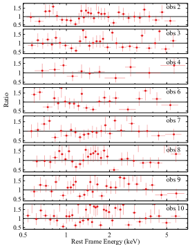
In this section, we conduct X-ray spectral analysis for KUG 1141. Before detailed modelling, we show X-ray spectra extracted from some of the observations in Fig. 3 to give an overview of the X-ray spectral variability in KUG 1141. The spectra are all unfolded using a power law with to remove the effects of instrumental response for demonstration purposes.
As shown in Fig. 3, the X-ray continuum of KUG 1141 shows a power-law shape with a steady increase of flux. In 2017, the X-ray flux during obs 11 reaches the highest level, and the X-ray continuum is the softest. For reference, a power law with would be a horizontal line in this figure. The latest observation (obs 12) in 2019 shows a slightly lower X-ray flux state than obs 11 with a harder X-ray continuum. The variability of the spectra agrees with the flux and X-ray softness variation shown in Fig. 2.
Detailed X-ray spectral analysis and SED modelling in the later section are all conducted in XSPEC (v.12.10.1f, Arnaud, 1996). The line-of-sight Galactic absorption towards KUG 1141 is cm-2, and the Galactic extinction is (Willingale et al., 2013). The tbnew (Wilms et al., 2000) and the zdust (Pei, 1992) models in XSPEC are used for the Galactic X-ray absorption and optical/UV extinction. Their values are all fixed during the spectral fitting. A simple convolution model zmshift in XSPEC is used to account for the source redshift (z=0.038).
In the rest of this section, we start with analysing the XMM-Newton (obs 5) and the NuSTAR observations (obs 12) of KUG 1141, which have higher signal-to-noise than Swift XRT observations. A simultaneous Swift snapshot observation is considered for obs 12. In the end of this section, we present the analysis of all the Swift XRT observations.
| Obs No. | Parameter | Unit | Model 1 | Model 2 |
|---|---|---|---|---|
| 5 | - | |||
| XMM | Ecut | keV | 500 | 500 |
| keV | - | |||
| norm | - | unconstrained | ||
| - | 155.12/164 | 149.03/162 | ||
| 12 | - | |||
| NuSTAR | Ecut | keV | >220 | >90 |
| & Swift | kT | keV | - | |
| norm | - | |||
| - | 427.43/402 | 413.16/400 | ||
| 1 | - | |||
| Swift | Ecut | keV | 500 | 500 |
| kT | keV | - | 0.10 | |
| norm | - | |||
| - | 20.69/20 | 20.60/19 | ||
| 11 | - | |||
| Swift | Ecut | keV | 500 | 500 |
| kT | keV | - | 0.10 | |
| norm | - | |||
| - | 27.88/15 | 27.60/14 |
4.1 XMM-Newton (obs 5)


We first model the three EPIC spectra of obs 5 with an absorbed power-law model cutoffpl (Model 1). Due to the lack of simultaneous hard X-ray observation, we fix the high energy cutoff parameter at 500 keV. Model 1 is able to fit the EPIC spectra very well with . The best-fit parameters are shown in Table 2, and the corresponding ratio plot is shown in Fig. 4. \textcolorblackWe did not find obvious evidence for narrow emission feature or absorption edge features in the iron band.
In order to test for possible soft excess emission, we add an additional bbody model (Model 2), which improves the fit by only with 2 more parameters. See the left panel of Fig. 4 for comparison of the fits. Only an upper limit of the temperature parameter is obtained (<0.2 keV). The normalization parameter of the bbody model is not constrained. A contour plot of distribution on the vs. normalization parameter plane is shown in the right panel of Fig. 4. The normalization of the bbody component is consistent with a very low value, e.g. <, within a 3 uncertainty range. When is at a very low value, e.g. <0.07 keV, the fit is no longer sensitive to due to the lower limit of the energy coverage of EPIC.
We also test for any extra absorption along the line of the sight towards KUG 1141 by adding an additional tbnew model at the source redshift. We only obtain an upper limit of the column density (a 90% confidence range of cm-2).
To sum up, we conclude that the X-ray spectra of KUG 1141 during obs 5 are consistent with a Galactic-absorbed power law. There is no/little evidence for soft excess emission or additional line-of-sight absorption.
4.2 NuSTAR (obs 12)


4.2.1 Continuum emission
We first follow the approach in Section 4.1 by modelling the FPM and simultaneous XRT spectra of obs 12 with cutoffpl (Model 1). The best-fit parameters are shown in Table 2. A power law with a high energy cutoff of >220 keV is able to describe the spectra very well above 1 keV. \textcolorblackSimilar to XMM-Newton spectra, we did not find obvious evidence for any narrow emission line or absorption edge in the iron band of FPM spectra. Therefore, we conclude that the spectra have no or little contribution from any distant cold reflector.
However, we find clear evidence for soft excess emission below 1 keV (see the left top panel of Fig. 5). An additional bbody model for the soft excess emission (Model 2) can improve the fit by with 2 more free parameters. The constraint of the parameters of the bbody component is shown in the right panel of Fig. 5. The best-fit is keV, which is similar to the typical value for other Sy1s (e.g. Walter & Fink, 1993). Such soft excess emission is however not found in the XMM-Newton observation (obs 5) in 2009. Note that Model 2 requires a slightly harder continuum () with a smaller lower limit of the high energy cutoff (>90 keV) than Model 1.
4.2.2 Ultra-fast outflow?
We also notice that there is evidence for a weak narrow absorption line between 9–10 keV in both the FPMA and FPMB spectra of obs 12. The black arrows in the left panels of Fig. 5 show the position of the line. This feature is often interpreted as a blueshifted Fe xxv or Fe xxvi line from an ultra-fast outflow (e.g. Tombesi et al., 2011). By modelling the absorption line feature with the zgauss model, we obtain the best-fit line energy of keV at the source frame, line width of keV, equivalent width of eV. This additional line model is able to improve the fit by with 3 more parameters, corresponding to a F-statistic value of 4.3 with probability of 0.005.

We construct a photo-ionisation absorption grid model by using xstar (Kallman & Bautista, 2001) assuming a power-law illuminating spectrum with . Solar abundances are assumed. A turbulent velocity of 2000 km s-1 is used. The free parameters are the column density (), the ionisation state of the absorber (), and the blueshift parameter (). By modelling the absorption line with xstar, we obtain cm-2, and . The value of is calculated in the observer’s frame, which corresponds to a line-of-sight velocity of .
According to the best-fit xstar model, the absorption line at 9.72 keV is mainly Fe xxvi line with a little contribution from the Fe xxv line. See Fig. 6 for the best-fit absorption model. FPMs are unable to resolve these two lines due to their limited energy resolution. There was no simultaneous high resolution observation in soft X-rays, e.g. from XMM-Newton RGS or Chandra LEGT. Thus, we are also unable to check for blueshifted O vii line as predicted by our model. To sum up, we only point out the tentative evidence for an ultra-fast outflow with line-of-sight velocity of during obs 12, which was taken when KUG 1141 is in a high X-ray and optical/UV flux state.
4.3 Swift

4.3.1 Two extreme flux states: Obs 1 and 11
Obs 1 and obs 11 were taken by Swift in 2007 and 2017. During these two observations, KUG 1141 shows respectively the historical lowest and the highest X-ray flux states in the Swift archive.
We first model the XRT spectra of these two observations with cutoffpl with fixed at 500 keV. The best-fit values are shown in Table 2, and the corresponding ratio plots are shown in the left two panels of Fig. 7. The absorbed power-law models are able to describe the data very well with for obs 1 and for obs 11. The best-fit photon indices for obs 1 and 11 are and respectively, suggesting a softer X-ray continuum in the highest flux state than in the lowest flux state.
Alternatively, the spectral difference between obs 11 and obs 1, as shown in the middle panel of Fig. 3, might be due to not only a change in the intrinsic flux but also a variable line-of-sight column density. For example, we fit the spectrum of obs 1 with an additional neutral absorption model tbnew at the source redshift. The photon index of the power-law continuum is fixed at the best-fit value for obs 11 (). An additional absorber with a column density of cm-2 is then required to fit the spectrum of obs 1. Such a model also provides a good fit with . In this scenario, the intrinsic X-ray continuum emission of KUG 1141 remains similar steepness with only an increase of flux from 2007 to 2017. An additional variable Compton-thin absorber is required to explain the spectral variation. However, it is important to point out that the XMM-Newton observation (obs 5), which was also taken in a low flux state, rules out the possibility of such an absorber (see Section 4.1). Therefore, we conclude that the scenario of variable intrinsic continuum emission is preferred rather than a Compton-thin absorber crossing the line of sight in coincidence with a change in the intrinsic X-ray flux.
Second, as shown in Fig. 7, there is no significant evidence for soft excess emission. We here put an upper limit of the soft excess by assuming the best-fit given by obs 12 ( keV, see Section 4.2.1). We show vs. the normalization of the bbody model component for obs 1 and obs 11 in the right panel of Fig. 7. We obtain an upper limit of and for obs 1 and obs 11 respectively. The inclusion of such weak components does not affect the power-law continuum modelling (see Table 2 for comparison of Model 1 and 2). In summary, we find no evidence of soft excess emission in these two Swift observations of KUG 1141.
4.3.2 Other Swift observations
| Obs No. | ||
|---|---|---|
| 2 | 27.92/31 | |
| 3 | 32.25/29 | |
| 4 | 4.12/9 | |
| 6 | 24.32/21 | |
| 7 | 15.30/23 | |
| 8 | 31.63/30 | |
| 9 | 32.36/30 | |
| 10 | 49.59/40 |
Following the conclusions above, we model the XRT spectra extracted from the other Swift observations using an absorbed power-law model by following the same approach. The best-fit parameters are shown in Table 3, and the corresponding ratio plots can be found in Fig. 12. Similarly, we do not find statistically significant evidence for soft excess in these observations. The best-fit photon index shows a slightly increase with the observed X-ray flux from in 2007 to in 2014. However, the values are statistically consistent within a 90% confidence range. By comparing these Swift observations before 2015 with obs 11 in 2017, we find that the intrinsic continuum emission of KUG 1141 is significantly softer in the highest X-ray flux state ().
5 Multi-Wavelength SED Analysis
So far, we have obtained the best-fit models for the X-ray continuum emission in all the epochs. We find that the X-ray spectra of obs 1-11 all show a power-law shape. Only obs 12 shows weak soft excess emission below 1 keV, which is consistent with a blackbody with keV. No significant evidence of soft excess emission is found in the soft X-ray band of other epochs. No additional line-of-sight absorption was found during obs 5 (XMM-Newton) when the source was in a low flux state and obs 12 (NuSTAR and Swift) when the source was in a high flux state. In this section, we model the multi-wavelength SEDs of KUG 1141 in all the epochs with simultaneous observations from UVOT or OM (obs 4-12).
5.1 SED Modelling

We first model the disc thermal emission of KUG 1141 using the diskbb model. This model assumes a thin disc temperature profile of and has two parameters: the inner temperature of the disc () and the normalization parameter. The normalization parameter is defined as , where is the ‘apparent’ inner radius of the disc in km, is the source distance in 10 kpc, and is the inclination angle of the disc. See Section 5.2 for more discussion concerning the normalization parameter of diskbb. Note that both and the normalization parameter can change the total flux of the model.
Secondly, we calculate the Comptonisation spectrum of the hot coronal region using the convolution model simpl (Steiner et al., 2009). The simpl model calculates a power law-shaped Comptonisation spectrum that self-consistently accounts for the fraction of scattered radiation. The spectrum of the seed photons is the diskbb model as described above. In this way, we are able to constrain the strength of the disc thermal emission by consistently considering the scattering process, and thus estimate the inner radius of the disc (). Such a method was previously used to measure in BH transients when the sources are not necessarily in a thermal-dominant state (e.g. Steiner et al., 2009). The free parameters are the scattering fraction and the photon index of the power-law continuum ().
The total model is tbnew * zdust * zmshift * ( simpl * diskbb ) in the XSPEC format. Such a model can describe the SEDs of most epochs very well except obs 12. An additional weak bbody model is used to model the soft excess shown in obs 12 as demonstrated in Section 4.2.1. The best-fit SED models are shown in Fig. 8, and the best-fit parameters are shown in Table 10 and Fig. 9. In the top panel of Fig. 9, we also show the absorption-corrected broad band flux calculated between 0.01 eV–100 keV using our best-fit AGN component. The following conclusions can be drawn from our SED modelling:
1) An increase of the disc temperature together with an increase of the broad band flux is clearly seen according to our SED modelling. \textcolorblackFor instance, the best-fit inner temperature of the disc is eV during obs 4; a higher temperature of eV is required for obs 11. See the bottom middle panel of Fig. 8 for comparison of these two epochs. The increase of the disc temperature is able to explain the variability of the optical–UV continuum: the UV emission is more sensitive to the increase of the disc temperature than the optical emission, and thus increases by a larger factor than the optical emission as shown in fifth panel of Fig. 2.
2) \textcolorblackDespite an increase of the disc temperature, the normalization of the diskbb model decreases from in 2009 to in 2019. Note that, again, an increase of either or the normalization parameter can increase the flux of the model. The decrease of the normalization parameter suggests a decreasing inner radius of the disc as this parameter is proportional to . See Section 5.2 for more discussion concerning the inner radius of the disc.
3) The scattering fraction parameter () shows the number fraction of the disc seed photons that are up-scattered to the X-ray band in the coronal region and gives a physical interpretation of the X-ray–UV ratio shown in Fig. 2. is the highest during obs 11, where the X-ray flux and the X-ray–UV ratio are both shown to be the highest among all the epochs. It is interesting to note that the best-fit for obs 12 is similar to the values for obs 4-10 when the source is in a much lower UV and optical flux state.
A change in the coronal region might be a possible explanation: during the high flux state during obs 11, a different corona, e.g. of a larger size in which more disc seed photons are up-scattered, might exist. Therefore, a high fraction of accretion power is released in the form of non-thermal X-ray emission rather than the thermal emission from the disc during obs 11. The corona during obs 12 might however be similar to those during obs 4-10 despite a higher mass accretion rate. Our studies suggest that the X-ray–UV ratio/ do not necessarily show strict correlation with mass accretion rate in an individual AGN.
4) The photon index of the X-ray continuum () changes with . This suggests that the optical depth of the corona is sensitive to not only the mass accretion rate as shown by statistical studies of AGN surveys (e.g. Brightman et al., 2013) but also the energy interplay between the disc and the corona.
5.2 Estimating and
Assuming and a BH mass of 666 Oh et al. (2015) estimated (statistical error) for KUG 1141 based on the study of H emission line by following the method in Greene & Ho (2005). Systematic errors of this method can lead to a larger uncertainity range, such as the relation between and (Greene & Ho, 2005) and the uncertain geometry of the broad-line region (Kaspi et al., 2000; McLure & Dunlop, 2004). , we estimate the Eddington ratio of KUG 1141 in the past decade. For example, \textcolorblacka broad band flux of erg cm-2 s-1 during obs 4 corresponds to an Eddington ratio of . Our best-fit SED model suggests that the bolometric luminosity of KUG 1141 increases from of the Eddington limit in 2009 to in 2019. A similar fraction of mass accretion rate increase has also been seen in other flaring AGN (e.g. NGC 1566, Parker et al., 2019).
From the normalization parameter of the diskbb model, we are also able to estimate the inner radius of the disc. This parameter is defined as as introduced above, where is the ‘apparent’ inner radius. We assume a correction factor of 0.412 (Kubota et al., 1998) to convert to the real inner radius . For instance, \textcolorblackassuming a viewing angle of , the best-fit normalization parameter of diskbb for obs 4 is corresponding to an inner radius of . Based on our calculations, the inner disc radius of KUG 1141 decreases from 8 in 2009 to 3 in 2017 and 2019 assuming . An assumption for a higher viewing angle leads to a larger estimated value: decreases from 20 in 2009 to 8 in 2019 assuming . However, KUG 1141 is a Sy1 galaxy which is unlikely to be viewed from an edge-on angle according to the standard model of AGN (e.g. Antonucci, 1993) assuming the torus plane and the optical-emitting disc plane share the same inclination.
blackIn conclusion, we find evidence for a possible decreasing inner radius simultaneously with an increasing mass accretion rate in KUG 1141, and the value has decreased by a factor of approximately 2.7. The assumptions on viewing angle and black hole mass do not affect the change of parameters we observe but only the absolute values.

6 Discussion
6.1 The Behaviour of the Disc in KUG 1141
Runco et al. (2016) studied the SDSS and Keck observations of KUG 1141 in the optical band, which were taken respectively in 2005 and 2009. These optical spectra of KUG 1141 are consistent with a typical Sy1. Meanwhile, these two observations are mostly consistent, which suggests that the disc of KUG 1141 does not show large variability in the period of 2005-2009.
By analysing the observations after 2009, we find that KUG 1141 has shown a steady increase of optical and UV flux. The luminosity of KUG 1141 increases from 0.6% of the Eddington limit in 2009 to 3.2% in 2017. The latest UVOT observation suggests that UV and optical flux of KUG 1141 is still increasing.
Detailed SED modelling shows that the inner radius of the disc () in KUG 1141 decreases by a factor of approximately . \textcolorblackThe exact value of depends on the assumption for the disc inclination angle: decreases, for example, from 8 (20 ) in 2009 to 3 (8 ) in 2019 assuming (). Saxton et al. (2015) estimated the filling time of a truncated thin disc in the framework of the standard thin disc model (Shakura & Sunyaev, 1973). They found that, for example, it takes more than 800 years to refill a truncated disc with around a BH as in KUG 1141 based on viscous timescales. Therefore, the change of in KUG 1141 is much faster than expected.
The mechanisms behind a quick boost of mass accretion rate as in KUG 1141 are also still unclear. It might be related to the instability of a gas pressure-dominated disc at a low Eddington ratio (Saxton et al., 2015), the propagation process in the disc (e.g. Ross et al., 2018) or tidal disruption events (TDEs, Rees, 1988).
In the case of TDEs, it is interesting to note that theoretically the rise time for a TDE to reach the peak luminosity is less than 1 year, assuming a 1 star disrupted by a BH as in KUG 1141371 and the tidal radius is twice the periastron radius (De Colle et al., 2012). Indeed similar conclusions have been found in TDEs that have been very well monitored before their peak luminosity (e.g. Bade et al., 1996; Cenko et al., 2012; Arcavi et al., 2014). However, KUG 1141 has shown a steady flux increase in the past decade.
Moreover, there are three typical types of TDE X-ray spectra: 1) strong thermal emission (e.g. ASASSN-14li, Grupe et al., 2015); 2) very soft power-law continuum (e.g. in XMMSL2 J144605.0685735, Saxton et al., 2019); 3) hard power-law continuum (e.g. in Swift J164449.3573451, Burrows et al., 2011). The spectra of KUG 1141 do not agree with the former two types but only the third type of TDEs, which is only found in radio-loud galaxies with significant jet emission in X-rays. This is however not the case for KUG 1141 where there is no obvious evidence for radio emission from KUG 1141 in the VLA FIRST Survey (Wadadekar, 2004). Therefore, the increase of the mass accretion rate in KUG 1141 is unlikely due to TDEs, or KUG 1141 is at least not consistent with typical TDEs we have observed.
6.2 Comparison to BH Transient State Changes

In this section, we discuss possible connection between KUG 1141 and BH transients in outburst. BH transients are binary systems where the central accretors are stellar-mass BHs. The existence of two different flux states in these sources have been realised for decades (e.g. Oda et al., 1971). Their X-ray spectra can change from a soft spectrum characterised by a strong thermal component to a hard spectrum characterised by a power-law component. Such a transition is commonly seen during an outburst of a transient and shows a ‘Q’-shaped pattern in the X-ray hardness-intensity diagram (e.g. see a MAXI HID of GX 3394 in Jiang et al., 2019a).
Similarly, we show the HID for KUG 1141 in Fig. 10. The circles in the figure represent Swift observations, and the square represents the XMM-Newton observation in 2009. The ‘intensity’ is the total absorption-corrected AGN flux in the 0.01 eV–100 keV band given by the best-fit SED models. The thermal emission from the disc in AGN is in the optical and UV bands. Therefore, we show X-ray–UV ratio, which we calculate in Section 3, in the diagram as ‘hardness’ instead of X-ray hardness as for BH transients.
As shown in Fig. 10, KUG 1141 starts from the bottom right corner of the diagram in 2009 when the UV, optical and X-ray emission is all at a low flux level. Then the total luminosity of KUG 1141 starts increasing in 2014 while the X-ray–UV ratio still remains consistent. When the source reaches the highest X-ray flux state in 2017, a lower X-ray–UV ratio is found. The latest observation in 2019 shows that the UV and optical flux is still increasing. The current state of KUG 1141 is near the top left corner of the HID. Such a pattern is very similar to the ‘Q’-shaped HID of many BH transients in outburst.
blackThe latest Swift and NuSTAR observation of KUG 1141 (obs 12) suggests a hard X-ray continuum of at a high accretion rate. The combination of a hard X-ray power-law emission and strong disc thermal emission makes obs 12 of KUG 1141 a similar case to the intermediate state seen in some outbursts of BH transients. During these states, a stellar-mass BH transient often shows a modest mass accretion rate of , and the disc thermal component and the non-thermal power-law component of make similar contribution to the X-ray emission (e.g. GRS 1716249, Jiang et al., 2020a).
blackBesides, the outbursts of BH transients can last for various timescales, e.g. weeks (e.g. MAXI 1659152, Negoro et al., 2010) or years (e.g. Swift J1753.50127, Soleri et al., 2013). The corresponding lengths for a flaring AGN scaled by BH mass are much longer than observable timescales, e.g. years. Therefore, sources like KUG 1141 can show an outburst with a significant increase of accretion rate similar to a BH transient on very short timescales are very intriguing.
Last but not least, a persistent radio jet is often seen during the hard state observations of BH transients (e.g. Fender et al., 2005) while a quenching of the radio emission is observed during the transition to the soft state (e.g. Fender et al., 1999). On contrary, KUG 1141 was not observed by the VLA FIRST survey (Wadadekar, 2004), which was taken before the transition shown in Fig. 10 started. If KUG 1141 indeed shows a BH transient-like outburst, our hypothesis would predict simultaneous variability in the radio emission. A radio monitoring program for KUG 1141 in future will be able to answer the question.
6.3 Comparison to Typical Changing-Look AGN
blackChanging-look AGN are rare cases of AGN, where the optical continuum flux increases or decreases and the broad emission lines appear or disappear within short time-scales. In previous studies, Noda & Done (2018) suggested that some ‘changing-look’ AGN may have strong radiation or magnetic pressure in the disc, which may shorten the state transitions in AGN that are similar to BH transients. Ruan et al. (2019) showed that the combined – evolution of two ‘changing-look’ AGN show a similar shape as KUG 1141 does in Fig. 10 with a similar increase of .
blackAll of these properties make KUG 1141 a similar case to changing-look AGN. However, it is also important to note that KUG 1141 does not seem to change ‘look’, e.g. Sy2 to Sy1, along with the boost of accretion rate: the XMM-Newton observation taken in 2009 when the source was in a low- state was able to rule out a Compton-thick scenario that is commonly seen in Sy2 AGN (Risaliti et al., 1999); during the high- state, e.g. obs 12 in 2019, the X-ray spectra of KUG 1141 still remained unobscured. Besides, the Keck observation in the optical band presented in Runco et al. (2016) showed that KUG 1141 already had a typical Sy1 spectrum in 2009 during the low- state777Our follow-up optical observations taken by Lijiang Observatory during the high- state will be presented in the second paper of this series..
6.4 The Puzzling Soft Excess Emission
We find strong evidence for soft excess below 1 keV only in obs 12 when KUG 1141 is in the high flux state (). By modelling the soft excess emission with a phenomenological blackbody model (bbody), we obtain keV, which is similar to the value of a typical Sy1 (e.g. Gierliński et al., 1999).
Noda & Done (2018) suggests that a rising soft excess should be seen when an AGN goes through a ‘changing-look’ phase with a modest mass accretion rate, e.g. . However, we are only able to obtain an upper limit of the soft excess emission in obs 11 taken in 2017 when the X-ray flux is the highest and the continuum is the softest. This is contrary to the example of Mrk 1018 given by Noda & Done (2018).
There are two most popular explanations for the origin of the soft excess emission in Sy galaxies: warm corona and relativistic disc reflection.
| Warm Corona Model | Parameter | Value | Reflection Model | Parameter | Value |
|---|---|---|---|---|---|
| nthcomp | (keV) | relconv | q | ||
| (deg) | |||||
| (eV) | () | <80 | |||
| norm | reflionx | /erg cm s-1) | |||
| simpl | (eV) | ||||
| diskbb | linked | norm | |||
| norm | <20 | ||||
| simpl | linked | ||||
| diskbb | linked | ||||
| norm | |||||
| 492.14/404 | 486.04/401 | ||||
| 12.0 | 10.9 |
6.4.1 Warm corona
In the warm corona scenario, the Comptonisation spectrum from an optically thick corona () with a relatively low temperature of keV is used to explain the soft excess emission (e.g. Petrucci et al., 2018). This additional corona has a much lower temperature than the ‘hot corona’, and thus is called ‘warm corona’. \textcolorblackIn order to test for this model, we calculate the warm coronal emission by using the Comptonisation model nthcomp. A disc blackbody-shaped seed photon spectrum is considered in consistency with the thermal disc component diskbb. The temperature parameter for the seed photon spectrum in nthcomp is linked to the corresponding parameter of the diskbb model. The total model is tbnew * zdust * (nthcomp + simpl*diskbb). The best-fit parameters are shown in Table 4, and the best-fit model is shown in the top left panel of Fig. 11. Corresponding data/model ratio plots are shown in the bottom left panel of Fig. 11.
blackAccording to our warm corona-based SED model, the extreme UV emission (0.02 eV–0.2 keV) of KUG 1141 is dominated by the warm coronal emission. Consequently, a higher bolometric luminosity is predicted by this model ( erg cm-2 s-1 in the 0.01 eV–100 keV band corresponding to an Eddington ratio of ).
blackSimilar conclusions are achieved in other warm corona-based analyses of narrow-line Sy1s (e.g. Jin et al., 2017) and ‘changing-look’ AGN (e.g. Noda & Done, 2018), where they also find the emission at longer wavelength dominated by warm coronal emission. For instance, Noda & Done (2018) modelled the variable soft excess in the ‘changing-look’ AGN Mrk 1018 with warm corona models, and concluded that the phase transition between Sy1 and Sy1.9 in Mrk 1018 is controlled by the variable warm Comptonisation region. It is interesting to note that, in comparison, KUG 1141 only shows evidence for weak soft excess in obs 12 but not in obs 11 when KUG 1141 is in the highest and the softest X-ray state and a high optical and UV flux state. We do not expect the extreme UV emission to switch completely between a thermal-dominant state to a non-thermal/warm corona-dominant state without much flux and spectral change as suggested by the warm corona model.
6.4.2 Disc reflection
blackIn the disc reflection scenario, the soft excess is explained by reflection from the innermost region of the disc (e.g. Crummy et al., 2006; Walton et al., 2013; Jiang et al., 2019b) within only 10-20 from the BH (e.g. Morgan et al., 2008; Reis et al., 2013; Chartas et al., 2017; Fabian et al., 2020). The decreasing inner radius inferred by our SED models in Section 5.2 also suggests a thin disc that is forming in the region very close to the ISCO. The soft excess may arise as part of the reflection spectrum from the inner disc.
blackIn order to test for reflection models, we replace the bbody model with an extended version of the ionised plasma model reflionx (Ross & Fabian, 1993). The illuminating spectrum of reflionx is calculated using nthcomp. A variable disc seed photon temperature is considered and linked to the inner temperature of the disc (Jiang et al., 2020b). The convolution model relconv is used to account for relativistic effects (Dauser et al., 2013). The best-fit parameters are shown in the last column of Table 4, and the best-fit model is shown in the top right panel of Fig. 11. Corresponding data/model ratio plots are shown in the lower panel.
blackThe relativistic reflection model provides an equally good fit as the warm corona model with and 3 more free parameters. The inclination angle of the disc is consistent with either a face-on () or a high-inclination () scenario within a 90% confidence uncertainty range. Due to the limited signal-to-noise, we are only able to obtain an upper limit of the inner radius of the disc ( ), which is statistically consistent with measurements in Section 5.2.
blackIn comparison with the warm corona model, the reflection model indicates stronger disc thermal emission in the optical and UV band (see the top two panels in Fig. 11). The properties of the thermal disc component and the up-scattering fraction in the hot coronal region are consistent with the results obtained by modelling the soft excess with a blackbody model as in Section 5. A similar Eddington ratio of is also obtained.
blackThe apparent absence of broad Fe K emission line in the data does not rule out of the disc reflection scenario especially when the soft excess emission is shown (e.g. Gallo, 2006; García et al., 2019; Jiang et al., 2020b). They might be related to, for example, 1) a low reflection fraction (); 2) strong relativistic effects; 3) certain properties of the disc, e.g. ionisation and density; 4) limited signal-to-noise of the data in the iron band.
blackIn the case of KUG 1141, it is important to note that our best-fit reflection model suggests a low- scenario during obs 12 of KUG 1141 despite the clear evidence of soft excess emission. For instance, the reflection component only takes 2% of the total flux in the iron band (4–8 keV). A similar is shown in the hard X-ray band (20–30 keV), where the Compton hump is shown. Therefore, the lack of clear evidence for broad Fe K emission line is possibly caused by the low- nature of the source during obs 12 and the limited signal-to-noise of the data. Observations by future missions in soft X-rays, e.g. Athena, in combination with high-sensitivity hard X-ray mission, e.g. HEX-P, will provide a unique opportunity to constrain the broad Fe K emission line and the Compton hump in a low- scenario as in KUG 1141.

7 Conclusions
In this work, we present multi-epoch X-ray spectral analysis and SED modelling of a Sy1 called KUG 1141. KUG 1141 shows a simultaneous steady flux increase in the optical and UV bands since 2009. For instance, the UVW1 flux of the AGN in KUG 1141 has increased by more than one order of magnitude during the latest Swift observation on 26th December, 2019 compared to the observation in 2009. It is interesting that the optical–UV continuum becomes flatter at a higher flux state, which can be explained by an increase of the temperature and the accretion rate in the disc.
The X-ray luminosity of KUG 1141 shows a steady increase by one order of magnitude from 2007 to 2017 as well. The broad band HID of KUG 1141 in the last decade is very similar to the X-ray HID of stellar-mass BH transients in outburst. Such a rapid boost of mass accretion rate makes KUG 1141 a very interesting source. \textcolorblackBy modelling multi-wavelength SEDs, the luminosity of KUG 1141 increases from of the Eddington limit in 2009 to 3.2% in 2019. Along with the rapid increase of mass accretion rate, a possible decreasing inner radius of the disc is suggested by our SED models. We only find obvious evidence of soft excess in the latest observation in 2019, during which KUG 1141 has an Eddington ratio of and the UV and optical flux is shown to be the highest.
DATA AVAILABILITY
The data underlying this article are available in the High Energy Astrophysics Science Archive Research Center (HEASARC), at https://heasarc.gsfc.nasa.gov.
Acknowledgements
This paper was written during the outbreak of COVID-19 in China in 2020. We would like to acknowledge the doctors and nurses who have been working day and night to ensure the safety of Chinese people during this period. JJ acknowledges support from the Tsinghua Astrophysics Outstanding Fellowship and the Tsinghua Shuimu Scholar Program. LCH acknowledges support from National Science Foundation of China (11721303, 11991052) and National Key R&D Program of China (2016YFA0400702). DJKB acknowledges support from Royal Society. ACF acknowledges support from ERC Advanced Grant (340442). CSR thanks the UK Science and Technology Facilities Council for support under the New Applicant grant ST/R000867/1, and the European Research Council for support under the European Union’s Horizon 2020 research and innovation programme (834203). MLP is supported by European Space Agency Research Fellowships. DJW acknowledges support from an STFC Ernest Rutherford Fellowship. This work made use of data from the NuSTAR mission, a project led by the California Institute of Technology, managed by the Jet Propulsion Laboratory, and funded by NASA. This research has made use of the NuSTAR Data Analysis Software (NuSTARDAS) jointly developed by the ASI Science Data Center and the California Institute of Technology. This work made use of data supplied by the UK Swift Science Data Centre at the University of Leicester. This project was also based on observations obtained with XMM-Newton, an ESA science mission with instruments and contributions directly funded by ESA Member States and NASA. This project has made use of the Science Analysis Software (SAS), an extensive suite to process the data collected by the XMM-Newton observatory.
References
- Antonucci (1993) Antonucci R., 1993, ARA&A, 31, 473
- Arcavi et al. (2014) Arcavi I., et al., 2014, ApJ, 793, 38
- Arnaud (1996) Arnaud K. A., 1996, in Jacoby G. H., Barnes J., eds, Astronomical Society of the Pacific Conference Series Vol. 101, Astronomical Data Analysis Software and Systems V. p. 17
- Bade et al. (1996) Bade N., Komossa S., Dahlem M., 1996, A&A, 309, L35
- Breeveld et al. (2010) Breeveld A. A., et al., 2010, MNRAS, 406, 1687
- Brightman et al. (2013) Brightman M., et al., 2013, MNRAS, 433, 2485
- Buisson et al. (2017) Buisson D. J. K., Lohfink A. M., Alston W. N., Fabian A. C., 2017, MNRAS, 464, 3194
- Burrows et al. (2011) Burrows D. N., et al., 2011, Nature, 476, 421
- Cenko et al. (2012) Cenko S. B., et al., 2012, ApJ, 753, 77
- Chartas et al. (2017) Chartas G., Krawczynski H., Zalesky L., Kochanek C. S., Dai X., Morgan C. W., Mosquera A., 2017, ApJ, 837, 26
- Cheng et al. (2019) Cheng H., Yuan W., Liu H.-Y., Breeveld A. A., Jin C., Liu B., 2019, MNRAS, 487, 3884
- Clavel et al. (1992) Clavel J., et al., 1992, ApJ, 393, 113
- Cohen et al. (1986) Cohen R. D., Rudy R. J., Puetter R. C., Ake T. B., Foltz C. B., 1986, ApJ, 311, 135
- Crummy et al. (2006) Crummy J., Fabian A. C., Gallo L., Ross R. R., 2006, MNRAS, 365, 1067
- Dauser et al. (2013) Dauser T., Garcia J., Wilms J., Böck M., Brenneman L. W., Falanga M., Fukumura K., Reynolds C. S., 2013, MNRAS, 430, 1694
- De Colle et al. (2012) De Colle F., Guillochon J., Naiman J., Ramirez-Ruiz E., 2012, ApJ, 760, 103
- Fabian et al. (2020) Fabian A. C., et al., 2020, MNRAS, 493, 2518
- Fender et al. (1999) Fender R., et al., 1999, ApJ, 519, L165
- Fender et al. (2005) Fender R., Belloni T., Gallo E., 2005, Ap&SS, 300, 1
- Gallo (2006) Gallo L. C., 2006, MNRAS, 368, 479
- Gallo et al. (2018) Gallo L. C., Blue D. M., Grupe D., Komossa S., Wilkins D. R., 2018, MNRAS, 478, 2557
- García et al. (2019) García J. A., et al., 2019, ApJ, 871, 88
- Gierliński et al. (1999) Gierliński M., Zdziarski A. A., Poutanen J., Coppi P. S., Ebisawa K., Johnson W. N., 1999, MNRAS, 309, 496
- Goodrich (1989) Goodrich R. W., 1989, ApJ, 342, 224
- Greene & Ho (2005) Greene J. E., Ho L. C., 2005, ApJ, 630, 122
- Grupe et al. (2015) Grupe D., Komossa S., Saxton R., 2015, ApJ, 803, L28
- Hutsemékers et al. (2017) Hutsemékers D., Agís González B., Sluse D., Ramos Almeida C., Acosta Pulido J. A., 2017, A&A, 604, L3
- Jiang et al. (2019a) Jiang J., Fabian A. C., Wang J., Walton D. J., García J. A., Parker M. L., Steiner J. F., Tomsick J. A., 2019a, MNRAS, 484, 1972
- Jiang et al. (2019b) Jiang J., et al., 2019b, MNRAS, 489, 3436
- Jiang et al. (2020a) Jiang J., Fürst F., Walton D. J., Parker M. L., Fabian A. C., 2020a, MNRAS, 492, 1947
- Jiang et al. (2020b) Jiang J., Gallo L. C., Fabian A. C., Parker M. L., Reynolds C. S., 2020b, MNRAS, 498, 3888
- Jin et al. (2017) Jin C., Done C., Ward M., Gardner E., 2017, MNRAS, 471, 706
- Kallman & Bautista (2001) Kallman T., Bautista M., 2001, ApJS, 133, 221
- Kaspi et al. (2000) Kaspi S., Smith P. S., Netzer H., Maoz D., Jannuzi B. T., Giveon U., 2000, ApJ, 533, 631
- Kelly et al. (2009) Kelly B. C., Bechtold J., Siemiginowska A., 2009, ApJ, 698, 895
- Khachikyan & Weedman (1971) Khachikyan É. Y., Weedman D. W., 1971, Astrophysics, 7, 231
- Koss et al. (2012) Koss M., Mushotzky R., Treister E., Veilleux S., Vasudevan R., Trippe M., 2012, ApJ, 746, L22
- Kubota et al. (1998) Kubota A., Tanaka Y., Makishima K., Ueda Y., Dotani T., Inoue H., Yamaoka K., 1998, PASJ, 50, 667
- Leighly et al. (2015) Leighly K. M., Cooper E., Grupe D., Terndrup D. M., Komossa S., 2015, The Astrophysical Journal, 809, L13
- MacLeod et al. (2010) MacLeod C. L., et al., 2010, ApJ, 721, 1014
- Marin (2017) Marin F., 2017, A&A, 607, A40
- McLure & Dunlop (2004) McLure R. J., Dunlop J. S., 2004, MNRAS, 352, 1390
- Moran et al. (2000) Moran E. C., Barth A. J., Kay L. E., Filippenko A. V., 2000, ApJ, 540, L73
- Morgan et al. (2008) Morgan C. W., Kochanek C. S., Dai X., Morgan N. D., Falco E. E., 2008, ApJ, 689, 755
- Negoro et al. (2010) Negoro H., et al., 2010, The Astronomer’s Telegram, 2873, 1
- Noda & Done (2018) Noda H., Done C., 2018, MNRAS, 480, 3898
- Oda et al. (1971) Oda M., Gorenstein P., Gursky H., Kellogg E., Schreier E., Tananbaum H., Giacconi R., 1971, ApJ, 166, L1
- Oh et al. (2015) Oh K., Yi S. K., Schawinski K., Koss M., Trakhtenbrot B., Soto K., 2015, ApJS, 219, 1
- Parker et al. (2019) Parker M. L., et al., 2019, MNRAS, 483, L88
- Pei (1992) Pei Y. C., 1992, ApJ, 395, 130
- Peng et al. (2002) Peng C. Y., Ho L. C., Impey C. D., Rix H.-W., 2002, AJ, 124, 266
- Peng et al. (2010) Peng C. Y., Ho L. C., Impey C. D., Rix H.-W., 2010, AJ, 139, 2097
- Penston & Perez (1984) Penston M. V., Perez E., 1984, MNRAS, 211, 33P
- Petrucci et al. (2018) Petrucci P. O., Ursini F., De Rosa A., Bianchi S., Cappi M., Matt G., Dadina M., Malzac J., 2018, A&A, 611, A59
- Poole et al. (2008) Poole T. S., et al., 2008, MNRAS, 383, 627
- Rees (1988) Rees M. J., 1988, Nature, 333, 523
- Reis et al. (2013) Reis R. C., Miller J. M., Reynolds M. T., Fabian A. C., Walton D. J., Cackett E., Steiner J. F., 2013, ApJ, 763, 48
- Ricci et al. (2016) Ricci C., et al., 2016, ApJ, 820, 5
- Risaliti et al. (1999) Risaliti G., Maiolino R., Salvati M., 1999, ApJ, 522, 157
- Ross & Fabian (1993) Ross R. R., Fabian A. C., 1993, MNRAS, 261, 74
- Ross et al. (2018) Ross N. P., et al., 2018, MNRAS, 480, 4468
- Ruan et al. (2019) Ruan J. J., Anderson S. F., Eracleous M., Green P. J., Haggard D., MacLeod C. L., Runnoe J. C., Sobolewska M. A., 2019, arXiv e-prints, p. arXiv:1909.04676
- Runco et al. (2016) Runco J. N., et al., 2016, ApJ, 821, 33
- Runnoe et al. (2016) Runnoe J. C., et al., 2016, MNRAS, 455, 1691
- Saxton et al. (2015) Saxton R. D., Motta S. E., Komossa S., Read A. M., 2015, MNRAS, 454, 2798
- Saxton et al. (2019) Saxton R. D., et al., 2019, A&A, 630, A98
- Seyfert (1943) Seyfert C. K., 1943, ApJ, 97, 28
- Shakura & Sunyaev (1973) Shakura N. I., Sunyaev R. A., 1973, A&A, 24, 337
- Shappee et al. (2014) Shappee B. J., et al., 2014, ApJ, 788, 48
- Soleri et al. (2013) Soleri P., et al., 2013, MNRAS, 429, 1244
- Steiner et al. (2009) Steiner J. F., Narayan R., McClintock J. E., Ebisawa K., 2009, PASP, 121, 1279
- Tohline & Osterbrock (1976) Tohline J. E., Osterbrock D. E., 1976, ApJ, 210, L117
- Tombesi et al. (2011) Tombesi F., Cappi M., Reeves J. N., Palumbo G. G. C., Braito V., Dadina M., 2011, ApJ, 742, 44
- Troyer et al. (2016) Troyer J., Starkey D., Cackett E. M., Bentz M. C., Goad M. R., Horne K., Seals J. E., 2016, MNRAS, 456, 4040
- Uttley et al. (2003) Uttley P., Edelson R., McHardy I. M., Peterson B. M., Markowitz A., 2003, ApJ, 584, L53
- Vasudevan et al. (2009) Vasudevan R. V., Mushotzky R. F., Winter L. M., Fabian A. C., 2009, MNRAS, 399, 1553
- Vignali et al. (2003) Vignali C., et al., 2003, AJ, 125, 2876
- Wadadekar (2004) Wadadekar Y., 2004, A&A, 416, 35
- Walter & Fink (1993) Walter R., Fink H. H., 1993, A&A, 274, 105
- Walton et al. (2013) Walton D. J., Nardini E., Fabian A. C., Gallo L. C., Reis R. C., 2013, MNRAS, 428, 2901
- Willingale et al. (2013) Willingale R., Starling R. L. C., Beardmore A. P., Tanvir N. R., O’Brien P. T., 2013, MNRAS, 431, 394
- Wilms et al. (2000) Wilms J., Allen A., McCray R., 2000, ApJ, 542, 914
Appendix A Error estimation on the UVOT photometric measurements
blackHere we briefly introduce our methods on the error estimation for the UVOT photometric measurements. Given that the image decomposition procedures are only implemented on the optical images, we take two different strategies for UV and optical data respectively.
blackFor the photometric uncertainties in three UV filters (UVW1, UVM2, and UVW2), we simply adopt the measurements returned by the UVOTSOURCE tool, including both systematic and statistical errors. The systematic errors mainly refer to the uncertainties on the zero-point and the conversion from counts to flux (depending on the assumed spectral shape), and are added in quadrature to the statistical errors in the calculation of the total errors (Poole et al., 2008; Breeveld et al., 2010).
blackThe estimation of the uncertainties for AGN fluxes at longer wavelengths (V, B, and U filters) are addressed in a different way, as the errors in the image decomposition procedure needs to be taken into account. One of the highlights in our work is that a similar image decomposition procedure was carried out on the same object in multiple observations. Therefore, it is doable to obtain an error of the host galaxy flux from (some of) these measurements and assess the error of the AGN flux through the ‘error propagation formula’.
blackA straightforward relation between the observed flux is that
| (1) |
in which is the flux for the whole galaxy, including the AGN emission , the host starlight and the background . With the error propagation formula we can get
| (2) |
note that can be neglected. Therefore, can be obtained by calculating and .
black is estimated from the multiple image fitting results. We can get the averaged flux density and its standard deviation at the (observed) frequency , by
black
| (3) |
| (4) |
blackTable 5 lists the photometry for the host galaxy starlight for the eight UVOT observations in three optical bands, as well as the averaged flux densities and 1 errors.
black is estimated by using the UVOTSOURCE tool. Compared to the aperture utilized in the UV bands (5 arcsec), a larger aperture of 15 arcsec is employed. The results are listed in Table 6. With Equation 2, the errors of the AGN emission in three optical bands can be obtained. The photometric uncertainties utilized in the spectral fitting are summarized in Table 8, containing those in all the six UVOT filters.
blackOne thing should be pointed out that above method for the error estimation of the optical data is based on the premise that the model employed in the image fitting, i.e. ‘PSF + exponential-disc + background’ is the true model for the description of the light distribution of KUG 1141. Therefore, the estimated errors does not contain those arising from the deviations of the model from the reality, i.e. an extra component may need to be included, such as a bulge/bar. Due to the low spatial resolution of the UVOT images, to thoroughly address this issue is beyond the scope of this paper.
| Obs No. | , V | , B | , U |
|---|---|---|---|
| 4 | 2.95 | 1.44 | 0.35 |
| 6 | 2.50 | 1.67 | - |
| 7 | 2.42 | 1.57 | 0.37 |
| 8 | 2.10 | 1.10 | 0.25 |
| 9 | 2.41 | 1.25 | 0.38 |
| 10 | 2.15 | 1.17 | 0.28 |
| 11 | 2.68 | 1.18 | 0.38 |
| 12 | 2.72 | 1.25 | 0.36 |
| 2.49 | 1.33 | 0.34 | |
| 0.10 | 0.07 | 0.02 |
| Obs No. | , V | , B | , U |
|---|---|---|---|
| 4 | 0.11 | 0.05 | 0.02 |
| 6 | 0.13 | 0.06 | 0.03 |
| 7 | 0.16 | 0.07 | 0.04 |
| 8 | 0.12 | 0.06 | 0.03 |
| 9 | 0.11 | 0.05 | 0.03 |
| 10 | 0.15 | 0.07 | 0.03 |
| 11 | 0.14 | 0.07 | 0.05 |
| 12 | 0.15 | 0.08 | 0.06 |
| Obs No. | , V | , B | , U | , UVW1 | , UVM2 | , UVW2 |
|---|---|---|---|---|---|---|
| 4 | 0.78 | 0.47 | 0.25 | 0.19 | 0.13 | 0.12 |
| 6 | 0.74 | 0.45 | 0.49 | 0.37 | 0.27 | 0.24 |
| 7 | 0.88 | 0.46 | 0.42 | 0.35 | 0.27 | 0.24 |
| 8 | 0.64 | 0.51 | 0.48 | 0.36 | 0.26 | 0.24 |
| 9 | 0.88 | 0.47 | 0.48 | 0.37 | 0.26 | 0.23 |
| 10 | 1.26 | 1.14 | 1.07 | 0.79 | 0.62 | 0.56 |
| 11 | 1.35 | 1.21 | 1.45 | 1.24 | 1.07 | 1.01 |
| 12 | 1.59 | 1.53 | 1.64 | 1.59 | 1.21 | 1.23 |
| Obs No. | , V | , B | , U | , UVW1 | , UVM2 | , UVW2 |
|---|---|---|---|---|---|---|
| 4 | 0.15 | 0.09 | 0.03 | 0.01 | 0.01 | 0.01 |
| 6 | 0.17 | 0.09 | 0.04 | 0.02 | 0.01 | 0.01 |
| 7 | 0.19 | 0.10 | 0.04 | 0.01 | 0.02 | 0.01 |
| 8 | 0.16 | 0.09 | 0.03 | 0.02 | 0.01 | 0.01 |
| 9 | 0.15 | 0.09 | 0.03 | 0.02 | 0.01 | 0.01 |
| 10 | 0.18 | 0.10 | 0.04 | 0.04 | 0.02 | 0.02 |
| 11 | 0.17 | 0.10 | 0.05 | 0.05 | 0.03 | 0.03 |
| 12 | 0.18 | 0.11 | 0.06 | 0.06 | 0.04 | 0.04 |
Appendix B Additional Information of X-ray and SED Analysis
Detailed X-ray flux extracted from all the epochs is shown in Table 9 and visulised in Fig. 2. Data/model ratio plots for the Swift observations of KUG 1141 using an absorbed power law are shown in Fig. 12. The best-fit SED parameters for obs 4–12 are listed in Fig. 10 and visilised in Fig. 9.
| Obs No. | |||
|---|---|---|---|
| 1 | |||
| 2 | |||
| 3 | |||
| 4 | |||
| 5 | |||
| 6 | |||
| 7 | |||
| 8 | |||
| 9 | |||
| 10 | |||
| 11 | |||
| 12 |
| Obs | diskbb norm | |||||
|---|---|---|---|---|---|---|
| No. | eV | - | erg cm-2 s-1 | |||
| 4 | 2.0 | 19.13/13 | ||||
| 5 | 1.7 | 157.87/164 | ||||
| 6 | 3.2 | 44.68/25 | ||||
| 7 | 3.4 | 27.59/27 | ||||
| 8 | 3.4 | 48.23/34 | ||||
| 9 | 3.5 | 49.22/34 | ||||
| 10 | 6.3 | 60.88/44 | ||||
| 11 | 9.0 | 43.55/19 | ||||
| 12 | 10.9 | 489.81/405 |
Appendix C Short-Term Variability on Kilo-second Timescales

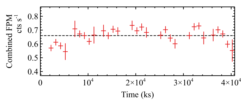
Fig. 13 and Fig. 14 show the XMM-Newton and NuSTAR lightcurves of KUG 1141extracted from obs 5 and 12. The gaps in the EPIC lightcurves are due to high flaring particle background. Both the X-ray and UV emission remains at a consistent flux level within this observation. This suggests that the multi-wavelength flux increase shown in Fig. 2 is not due to the lack of frequent monitoring of a very fast intrinsic AGN variability on timescales of kiloseconds.