The Average Rate of Convergence of the Exact Line Search Gradient Descent Method

Thomas Yu Department of Mathematics, Drexel University. Email: yut@drexel.edu. He is supported in part by the National Science Foundation grants DMS 1522337 and DMS 1913038.

(April 28, 2023
Revised March 5, 2024)

Abstract:

It is very well known that when the exact line search gradient descent method is applied to a convex quadratic objective, the worst-case rate of convergence (ROC), among all seed vectors, deteriorates as the condition number of the Hessian of the objective grows. By an elegant analysis due to H. Akaike, it is generally believed – but not proved – that in the ill-conditioned regime the ROC for almost all initial vectors, and hence also the average ROC, is close to the worst case ROC. We complete Akaike’s analysis using the theorem of center and stable manifolds. Our analysis also makes apparent the effect of an intermediate eigenvalue in the Hessian by establishing the following somewhat amusing result: In the absence of an intermediate eigenvalue, the average ROC gets arbitrarily fast – not slow – as the Hessian gets increasingly ill-conditioned.

We discuss in passing some contemporary applications of exact line search GD to polynomial optimization problems arising from imaging and data sciences.

Keywords: Gradient descent, exact line search, worst case versus average case rate of convergence, center and stable manifolds theorem, polynomial optimization problem

1 Introduction

Exact line search is usually deemed impractical in the optimization literature, but when the objective function has a specific global structure then its use can be beneficial. A notable case is when the objective is a polynomial. Polynomial optimization problems (POPs) abound in diverse applications; see, for example, [15, 13, 6, 4, 8, 14] and Section 1.2.

For the gradient descent (GD) method, a popular choice for the step size is $s=1/L$ , where $L$ is a Lipschitz constant satisfied by the gradient, i.e. $\|\nabla f(x)-\nabla f(y)\|\leq L\|x-y\|$ . The rate of convergence of GD would then partly depend on how well one can estimate $L$ . Exact line search refers to the ‘optimum’ choice of step size, namely $s=\mathop{\rm argmin}_{t}f(x+td)$ , where $d$ is the search direction, hence the nomenclature optimum gradient descent in the case of $d=-\nabla f(x)$ .¹¹1We use the terms ‘optimum GD’ and ‘GD with exact line search’ interchangeably in this article. When $f$ is, say, a degree 4 polynomial, it amounts to determining the univariate quartic polynomial $p(t)=f(x-td)$ followed by finding its minimizer, which is a very manageable computational task.

Let us recall the key benefit of exact line search. We focus on the case when the objective is a strictly convex quadratic, which locally approximates any smooth objective function in the vicinity of a local minimizer with a positive definite Hessian. By the invariance of GD (constant step size or exact line search) under rigid transformations, there is no loss of generality, as far as the study of ROC is concerned, to consider only quadratics of the form

\displaystyle f(x)=\frac{1}{2}x^{T}Ax,\mbox{ with }A={\rm diag}(\lambda),\;\;\lambda=(\lambda_{1},\ldots,\lambda_{n}),\;\;\lambda_{1}\geq\cdots\geq\lambda_{n}>0.

(1.1)

Its gradient is Lipschitz continuous with Lipschitz constant $L=\lambda_{1}$ . Also, it is strongly convex with the strong convexity parameter $\sigma=\lambda_{n}$ . In the case of constant step size GD, we have $x^{(k+1)}=(I-sA)x^{(k)}$ , so the rate of convergence is given the spectral radius of $I-sA$ , which equals $\max_{1\leq i\leq n}|1-s\lambda_{i}|$ . From this, it is easy to check that the step size

\displaystyle s=2/(\lambda_{1}+\lambda_{n})

(1.2)

minimizes the spectral radius of $I-sA$ , and hence offers the optimal ROC

\displaystyle\|x^{(k)}\|=O(\rho^{k})\mbox{ with }\;\rho=\frac{\lambda_{1}-\lambda_{n}}{\lambda_{1}+\lambda_{n}}.

(1.3)

Gradient descent with exact line search involves non-constant step sizes: $x^{(k+1)}=(I-s_{k}A)x^{(k)}$ , with $s_{k}=(x^{(k)})^{T}A^{2}x^{(k)}/(x^{(k)})^{T}A^{3}x^{(k)}$ . For convenience, denote the iteration operator by OGD, i.e.

\displaystyle x^{(k+1)}=\textsf{OGD}(x^{(k)}),\quad\textsf{OGD}(x):=\textsf{OGD}(x;\lambda):=x-\frac{x^{T}A^{2}x}{x^{T}A^{3}x}Ax.

(1.4)

We set $\textsf{OGD}(0)=0$ so that OGD is a well-defined self-map on $\mbox{$\mathbb{R}$}^{n}$ . By norm equivalence, one is free to choose any norm in the study of ROC; and the first trick is to notice that by choosing the $A$ -norm, defined by $\|x\|_{A}:=\sqrt{x^{T}Ax}$ , we have the following convenient relation:

\displaystyle\|\textsf{OGD}(x)\|_{A}^{2}=\left[1-\frac{(x^{T}A^{2}x)^{2}}{(x^{T}Ax)(x^{T}A^{3}x)}\right]\|x\|_{A}^{2}.

(1.5)

Write $d=Ax$ ( $=\nabla f(x)$ ). By the Kantorovich inequality,²²2For a proof of the Kantorovich inequality $\frac{(d^{T}d)^{2}}{(d^{T}A^{-1}d)(d^{T}Ad)}\geq\frac{4\lambda_{1}\lambda_{n}}{(\lambda_{1}+\lambda_{n})^{2}}=\frac{4{\rm cond}(A)}{(1+{\rm cond}(A))^{2}}$ , see, for example, [12, 7]. A good way to appreciate this result is to compare it with the following bound obtained from Rayleigh quotient: $\frac{(d^{T}d)^{2}}{(d^{T}A^{-1}d)(d^{T}Ad)}\geq\frac{\lambda_{n}}{\lambda_{1}}={\rm cond}(A)^{-1}$ . Unless $\lambda_{1}=\lambda_{n}$ , Kantorovich’s bound is always sharper, and is the sharpest possible in the sense that there exists a vector $d$ so that equality holds.

\displaystyle\frac{(x^{T}A^{2}x)^{2}}{(x^{T}Ax)(x^{T}A^{3}x)}=\frac{(d^{T}d)^{2}}{(d^{T}A^{-1}d)(d^{T}Ad)}\geq\frac{4\lambda_{1}\lambda_{n}}{(\lambda_{1}+\lambda_{n})^{2}},

(1.6)

which yields the well-known error bound for the optimum GD method:

\displaystyle\|x^{(k)}\|_{A}\leq\Big{(}\frac{\lambda_{1}-\lambda_{n}}{\lambda_{1}+\lambda_{n}}\Big{)}^{k}\|x^{(0)}\|_{A}.

(1.7)

So optimum GD satisfies the same upper-bound for its ROC as in (1.3). The constant step size GD method with the optimal choice of step size (1.2), however, should not be confused with the optimum GD method, they have the following fundamental differences:

•

The optimal step size (1.2) requires the knowledge of the two extremal eigenvalues, of which the determination is no easier than the original minimization problem. In contrast, the optimum GD method is blind to the values of $\lambda_{1}$ and $\lambda_{n}$ .
•

Due to the linearity of the iteration process, GD with the optimal constant step size (1.2) achieves the ROC $\|x^{(k)}\|\asymp C\rho^{k}$ , with $\rho$ in (1.3), for any initial vector with a non-zero component in the dominant eigenvector of $A$ , and hence for almost all initial vectors $x^{(0)}$ . So for this method the worst case ROC is the same as the average ROC. (As the ROC is invariant under scaling of $x^{(0)}$ , the average and worst case ROC can be defined by taking the average and maximum, respectively, ROC over all seed vectors of unit length.) In contrast, OGD is nonlinear and the worst case ROC (1.3) is attained only for specific initial vectors $x^{(0)}$ ; see Proposition 3.1. It is much less obvious how the average ROC, defined by (1.10) below, compares to the worst case ROC.

Due to (1.5), we define the (one-step) shrinking factor by

\displaystyle\rho(x,\lambda)=\sqrt{1-\frac{(x^{T}A^{2}x)^{2}}{(x^{T}Ax)(x^{T}A^{3}x)}}=\sqrt{1-\frac{(\sum_{i}\lambda_{i}^{2}x_{i}^{2})^{2}}{(\sum_{i}\lambda_{i}x_{i}^{2})(\sum_{i}\lambda_{i}^{3}x_{i}^{2})}}.

(1.8)

Then, for any initial vector $x^{(0)}\neq 0$ , the rate of convergence of the optimum gradient descent method applied to the minimization of (1.1) is given by

\displaystyle\rho^{\ast}(x^{(0)},\lambda):=\limsup_{k\rightarrow\infty}\Bigg{[}\prod_{j=0}^{k-1}\rho(\textsf{OGD}^{j}(x^{(0)}),\lambda)\Bigg{]}^{1/k}.

(1.9)

As $\rho^{\ast}(x^{(0)},\lambda)$ depends only on the direction of $x^{(0)}$ , and is insensitive to sign changes in the components of $x^{(0)}$ (see (2.1)), the average ROC can be defined based on averaging over all $x^{(0)}$ on the unit sphere, or just over the positive octant of the unit sphere. Formally,

Definition 1.1

The average ROC of the optimum GD method applied to (1.1) is

\displaystyle\mbox{Average ROC}:=\int_{\mbox{$\mathbb{S}$}^{n-1}}\rho^{\ast}(x,\lambda)d\mu(x)=2^{n}\int_{\mbox{$\mathbb{S}$}^{n-1}_{+}}\rho^{\ast}(x,\lambda)d\mu(x),

(1.10)

where $\mu$ is the uniform probability measure on $\mbox{$\mathbb{S}$}^{n-1}$ , and $\mbox{$\mathbb{S}$}^{n-1}_{+}:=\{x\in\mbox{$\mathbb{S}$}^{n-1}:x\geq 0\}$ .

We have

\displaystyle\mbox{Average ROC}\leq\mbox{Worst case ROC}\stackrel{{\scriptstyle(\ast)}}{{=}}\frac{1-a}{1+a},\;\;\;\mbox{ where }a=\frac{\lambda_{n}}{\lambda_{1}}={\rm cond}(A)^{-1}.

(1.11)

Note that (1.7) only shows that the worst case ROC is upper bounded by $(1-a)/(1+a)$ ; for a proof of the equality ( $\ast$ ) in (1.11), see Proposition 3.1.

1.1 Main results

In this paper, we establish the following result:

Theorem 1.2

(i) If $A$ has only two distinct eigenvalues, then the average ROC approaches 0 when ${\rm cond}(A)\rightarrow\infty$ . (ii) If $A$ has an intermediate eigenvalue $\lambda_{i}$ uniformly bounded away from the two extremal eigenvalues, then the average ROC approaches the worst case ROC in (1.11), which approaches 1, when ${\rm cond}(A)\rightarrow\infty$ .

The second part of Theorem 1.2 is an immediate corollary of the following result:

Theorem 1.3

If $A$ has an intermediate eigenvalue, i.e. $n>2$ and there exists $i\in\{2,\ldots,n-1\}$ s.t. $\lambda_{1}>\lambda_{i}>\lambda_{n}$ , then

\displaystyle\operatorname*{ess\,inf}_{x^{(0)}\in\mathbb{S}^{n-1}}\rho^{\ast}(x^{(0)},\lambda)=\frac{1-a}{\sqrt{(1+a)^{2}+Ba}},

(1.12)

where $a={\rm cond}(A)^{-1}$ , $B=\frac{4(1+\delta^{2})}{1-\delta^{2}}$ , $\delta=\min_{i:\lambda_{1}>\lambda_{i}>\lambda_{n}}\frac{\lambda_{i}-(\lambda_{1}+\lambda_{n})/2}{(\lambda_{1}-\lambda_{n})/2}$ .

Remark 1.4

It is shown in [5, §2] that $\rho^{\ast}(x^{(0)},\lambda)$ is lower-bounded by the right-hand side of (1.12) with the proviso of a difficult-to-verify condition on $x^{(0)}$ . The undesirable condition seems to be an artifact of the subtle argument in [5, §2], which also makes it hard to see whether the bound (1.12) is tight. Our proof of Theorem 1.3 uses Akaike’s results in [5, §1], but replace his arguments in [5, §2] by a more natural dynamical system approach. The proof shows that the bound is tight and holds for a set of $x^{(0)}$ of full measure, which also allows us to conclude the second part of Theorem 1.2. It uses the center and stable manifolds theorem, a result that was not available at the time [5] was written.

Remark 1.5

For constant step size GD, ill-conditioning alone is enough to cause slow convergence for almost all initial vectors. For exact line search, however, it is ill-conditioning in cahoot with an intermediate eigenvalue that causes the slowdown. This is already apparent from Akaike’s analysis; the first part of Theorem 1.2 intends to bring this point home, by showing that the exact opposite happens in the absence of an intermediate eigenvalue.

Organization of the proofs. In Section 2, we recall the results of Akaike, along with a few observations not directly found in [5]. These results and observations are necessary for the final proofs of Theorem 1.2(i) and Theorem 1.3, to be presented in Section 3 and Section 4, respectively. The key idea of Akaike is an interesting discrete dynamical system, with a probabilistic interpretation, underlying the optimum GD method. We give an exposition of this dynamical system in Section 2. A key property of this dynamical system is recorded in Theorem 2.2. In a nutshell, the theorem tells us that part of the properties of the dynamical system in the high-dimensional case is captured by the 2-dimensional case; so – while the final results say that there is a drastic difference between the $n=2$ and $n>2$ cases – the analysis of the latter case (in Section 4) uses some of the results in the former case (in Section 3). Appendix A records two auxiliary technical lemmas. Appendix B recalls a version of the theorem of center and stable manifolds stated in the monograph [17], and discusses a refinement of the result needed to prove the full version of Theorem 1.3.

Section 3 and Section 4 also present computations, in Figures 2 and 3, that serve to illustrate some key ideas behind the proofs.

Before proceeding to the proofs, we consider some contemporary applications of exact line search methods to POPs.

1.2 Applications of exact line search methods to POPs

In its abstract form, the phase retrieval problem seeks to recover a signal $x\in\mathbb{K}^{n}$ ( $\mathbb{K}=\mbox{$\mathbb{R}$}$ or $\mathbb{C}$ ) from its noisy ‘phaseless measurements’ $y_{i}\approx|\langle x,a_{i}\rangle|^{2}$ , with enough random ‘sensors’ $a_{i}\in\mathbb{K}^{n}$ . A plausible approach is to choose $x$ that solves

\displaystyle\min_{x\in\mathbb{K}^{n}}\sum_{j=1}^{m}\Big{[}y_{j}-|\langle x,a_{j}\rangle|^{2}\Big{]}^{2}.

(1.13)

The two squares makes it a degree 4 POP.

We consider also another data science problem: matrix completion. In this problem, we want to exploit the a priori low rank property of a data matrix $M$ in order to estimate it from just a small fraction of its entries $M_{i,j}$ , $(i,j)\in\Omega$ . If we know a priori that $M\in\mbox{$\mathbb{R}$}^{m\times n}$ has rank $r\ll\min(m,n)$ , then similar to (1.13) we may hope to recover $M$ by solving

\displaystyle\min_{X\in\mbox{$\mathbb{R}$}^{m\times r},Y\in\mbox{$\mathbb{R}$}^{n\times r}}\sum_{(i,j)\in\Omega}\Big{[}(XY^{T})_{i,j}-M_{i,j}\Big{]}^{2}.

(1.14)

It is again a degree 4 POP.

Extensive theories have been developed for addressing the following questions: (i) Under what conditions – in particular how big the sample size $m$ for phase retrieval and $|\Omega|$ for matrix completion – would the global minimizer of (1.13) or (1.14) recovers the underlying object of interest? (ii) What optimization algorithms would be able to compute the global minimizer?

It is shown in [13] that constant step size GD with an appropriate choice of initial vector and step size applied to the optimization problems above probably guarantees success in recovering the object of interest under suitable statistical models. For the phase retrieval problem, assume for simplicity $x^{\ast}\in\mbox{$\mathbb{R}$}^{n}$ , $y_{j}=(a_{j}^{T}x^{\ast})^{2}$ , write

\displaystyle f(x):=\frac{1}{4m}\sum_{j=1}^{m}\Big{[}y_{j}-(a_{j}^{T}x)^{2}\Big{]}^{2}.

(1.15)

Then

\displaystyle\nabla f(x)=-\frac{1}{m}\sum_{j=1}^{m}\Big{[}y_{j}-(a_{j}^{T}x)^{2}\Big{]}(a_{j}^{T}x)a_{j}\;\mbox{ and }\;\nabla^{2}f(x)=\frac{1}{m}\sum_{j=1}^{m}\Big{[}3(a_{j}^{T}x)^{2}-y_{j}\Big{]}a_{j}a_{j}^{T}.

(1.16)

Under the Gaussian design of sensors $a_{j}\stackrel{{\scriptstyle\rm i.i.d.}}{{\sim}}N(0,I_{n})$ , $1\leq j\leq m$ , considered in, e.g., [10, 9, 13], we have

\mathbb{E}\big{[}\nabla^{2}f(x)\big{]}=3\big{[}\|x\|_{2}^{2}I_{n}+2xx^{T}\big{]}-\big{[}\|x^{\ast}\|_{2}^{2}I_{n}+2x^{\ast}(x^{\ast})^{T}\big{]}.

At the global minimizer $x=x^{\ast}$ , $\mathbb{E}\big{[}\nabla^{2}f(x^{\ast})\big{]}=2\big{[}\|x^{\ast}\|_{2}^{2}I_{n}+2x^{\ast}(x^{\ast})^{T}\big{]}$ , so

{\rm cond}(\mathbb{E}\big{[}\nabla^{2}f(x^{\ast})\big{]})=3.

This suggests that when the sample size $m$ is large enough, we may expect that the Hessian of the objective is well-conditioned for $x\approx x^{\ast}$ . Indeed, when $m\asymp n\log n$ , the discussion in [13, Section 2.3] implies that ${\rm cond}(\nabla^{2}f(x^{\ast}))$ grows slowly with $n$ :

{\rm cond}(\nabla^{2}f(x^{\ast}))=O(\log n)

with a high probability. However, unlike (1.1), the objective (1.15) is a quartic instead of a quadratic polynomial, so the Hessian $\nabla^{2}f(x)$ is not constant in $x$ . We have the following phenomena:

(i)

On the one hand, in the directions given by $a_{j}$ , the Hessian $\nabla^{2}f(x^{\ast}+\delta a_{j}/\|a_{j}\|)$ has a condition number that grows (up to logarithmic factors) as $O(n)$ , meaning that the objective can get increasingly ill-conditioned as the dimension $n$ grows, even within a small ball around $x^{\ast}$ with a fixed radius $\delta$ .
(ii)

On the other hand, most directions $v$ would not be too close to be parallel to $a_{j}$ , and ${\rm cond}\big{(}\nabla^{2}f(x^{\ast}+\delta v/\|v\|)\big{)}=O(\log n)$ with a high probability.
(iii)

Constant step-size GD, with a step size that can be chosen nearly constant in $n$ , has the property of staying away from the ill-conditioned directions, hence no pessimistically small step sizes or explicit regularization steps avoiding the bad directions are needed. Such an ‘implicit regularization’ property of constant step size GD is the main theme of the article [13].

To illustrate (i) and (ii) numerically, we compute the condition numbers of the Hessians $\nabla^{2}f(x)$ at $x=x^{\ast}=\bar{x}/\|\bar{x}\|$ , $x=x^{\ast}+.5a_{1}/\|a_{1}\|$ and $x=x^{\ast}+.5z/\|z\|$ for $a_{j},\bar{x},z\stackrel{{\scriptstyle\rm i.i.d.}}{{\sim}}N(0,I_{n})$ , with $n=1000k$ , , $k=1,\ldots,5$ , and $m=n\log_{2}(n)$ :

	${\rm cond}(\nabla^{2}f(x^{\ast}))$	${\rm cond}(\nabla^{2}f(x^{\ast}+.5a_{1}/\\|a_{1})$	${\rm cond}(\nabla^{2}f(x^{\ast}+.5z/\\|z\\|))$
$n=1000$	14.1043	147.6565	17.2912, 16.0391, 16.7982
$n=2000$	12.1743	193.6791	15.3551, 14.9715, 14.5999
$n=3000$	11.4561	251.2571	14.3947, 13.8015, 14.0738
$n=4000$	11.5022	310.8092	13.9249, 13.6388, 13.5541
$n=5000$	10.8728	338.3008	13.2793, 12.9796, 13.3100

(The last column is based on three independent samples of $z\sim N(0,I_{n})$ .) Evidently, the condition numbers do not increase with the dimension $n$ in the first and third columns, while a near linear growth is observed in the second column.

We now illustrate (iii); moreover, we present experimental results suggesting that exact line search GD performs favorably compared to constant step size GD. For the latter, we first show how to efficiently compute the line search function $p(t):=f(x+td)$ by combining (1.15) and (1.16). Write $A=[a_{1},\cdots,a_{m}]\in\mbox{$\mathbb{R}$}^{n\times m}$ . We can compute the gradient descent direction together with the line search polynomial $p(t)$ by computing the following sequence of vectors and scalars, with the computational complexity of each listed in parenthesis:

	$\displaystyle(1)\;A^{T}x\;\;(\approx 2mn),\;\;\;(2)\;\alpha=-y+(A^{T}x)^{2}\;\;(O(m)),\;\;\;(3)\;d=-\nabla f(x)=-\frac{1}{m}A(\alpha\cdot A^{T}x)\;\;(\approx 2mn),$
	$\displaystyle(4)\;A^{T}d\;\;(\approx 2mn),\;\;\;(5)\;\beta=2(A^{T}x)\cdot(A^{T}d)\;\;(O(m)),\;\;\;(6)\;\gamma=(A^{T}d)^{2}\;\;(O(m))$
	$\displaystyle(7)\;\gamma^{T}\gamma,\;2\beta^{T}\gamma,\;\beta^{T}\beta+2\alpha^{T}\gamma,\;2\alpha^{T}\beta,\;\alpha^{T}\alpha\;\;(O(m))$
	$\displaystyle(8)\;s^{\ast}=\mathop{\rm argmin}_{t\geq 0}p(t),\;p(t)=f(x+td)=(\gamma^{T}\gamma)t^{4}+(2\beta^{T}\gamma)t^{3}+(\beta^{T}\beta+2\alpha^{T}\gamma)t^{2}+(2\alpha^{T}\beta)t+\alpha^{T}\alpha\;\;(O(1)).$

In above, $u\cdot v$ , for two vectors $u$ , $v$ of the same length, stands for componentwise multiplication, and $v^{2}:=v\cdot v$ . As we can see, the dominant steps are steps (1), (3) and (4). As only steps (1)-(3) are necessary for constant step size GD, we conclude that, for the phase retrieval problem, exact line search GD is about 50% more expensive per iteration than constant step size GD.

Figure 1 shows the rates of convergence for gradient descent with constant step size $s=0.1$ (suggested in [13, Section 1.4]) and exact line search for $n=10,100,200,1000,5000,10000$ , $m=10n$ , with the initial guess chosen by a so-called spectral initialization.³³3Under the Gaussian design $a_{1},\ldots,a_{m}\sim_{\rm i.i.d.}N(0,I_{n})$ , it is interesting to see that $E[(a_{i}^{T}x)^{2}a_{i}a_{i}^{T}]=I+2xx^{T}$ . As the Rayleigh quotient $u^{T}(I+2xx^{T})u/u^{T}u=1+2(u^{T}x)^{2}/u^{T}u$ is maximized when $u$ is parallel to $x$ , an educated initial guess for $x$ would be a suitably scaled dominant eigenvector of $\frac{1}{m}\sum_{r=1}^{m}y_{r}a_{r}a_{r}^{T}$ , which can be computed from the data $(y_{r})_{r=1}^{m}$ and sensors $(a_{r})_{r=1}^{m}$ using the power method. See, for example, [13, 9] for more details and references therein. As the plots show, for each signal size $n$ the ROC for exact line search GD is more than twice as fast as that of constant step size GD.

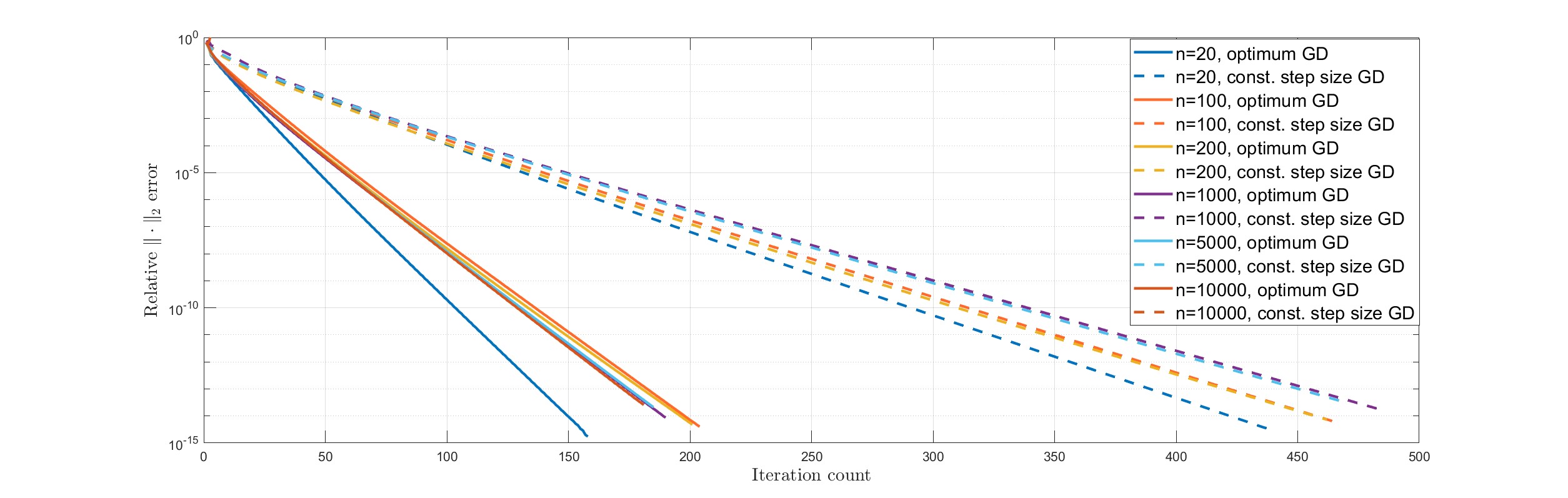Refer to caption — Figure 1: ROC of constant step size GD vs optimum GD for the phase retrieval problem

Not only is the speedup in ROC by exact line search outweighs the 50% increase in per-iteration cost, the determination of step size is automatic and requires no tuning. For each $n$ , the ROC for exact line search GD in Figure 1 is slightly faster than $O([(1-a)/(1+a)]^{k})$ for $a={\rm cond}(\nabla^{2}f(x^{\ast}))^{-1}$ – the ROC attained by optimum GD as if the degree 4 objective has a constant Hessian $\nabla^{2}f(x^{\ast})$ (Theorem 1.3)– suggesting also that the GD method implicitly avoids the ill-conditioned directions (recall the table above), akin to what is established in [13]. Unsurprisingly, our experiments also suggest that exact line search GD is more robust than its constant step size counterpart for different choices of initial vectors. Similar advantages for exact line search GD was observed for the matrix completion problem.

2 Properties of OGD and Akaike’s $T$

Let $\mbox{$\mathbb{R}$}^{n}_{\ast}$ be $\mbox{$\mathbb{R}$}^{n}$ with the origin removed. For $x\in\mbox{$\mathbb{R}$}^{n}$ , define $|x|\in\mbox{$\mathbb{R}$}^{n}$ by $|x|_{i}=|x_{i}|$ . Notice from (1.8) that, for a fixed $\lambda$ , $\rho(\cdot,\lambda)$ is invariant under both scaling and sign-changes of the components, i.e.

\displaystyle\begin{split}\rho(\alpha\mathcal{E}x,\lambda)=\rho(x,\lambda),\quad\forall x\in\mbox{$\mathbb{R}$}^{n}_{\ast},\;\alpha\neq 0,\;\mathcal{E}={\rm diag}(\varepsilon_{1},\ldots,\varepsilon_{n}),\;\varepsilon_{i}\in\{1,-1\}.\end{split}

(2.1)

In other words, $\rho(x,\lambda)$ depends only on the equivalence class $[x]_{\sim}$ , where $x\sim y$ if $|x|/\|x\|=|y|/\|y\|$ .

By inspecting (1.4) one sees that

\displaystyle\begin{split}\textsf{OGD}(\alpha\mathcal{E}x,\lambda)=\alpha\mathcal{E}\!\cdot\!\textsf{OGD}(x,\lambda),\quad\forall x\in\mbox{$\mathbb{R}$}^{n}_{\ast},\;\alpha\neq 0,\;\mathcal{E}={\rm diag}(\varepsilon_{1},\ldots,\varepsilon_{n}),\;\varepsilon_{i}\in\{1,-1\}.\end{split}

(2.2)

This means $[\textsf{OGD}(x)]_{\sim}$ , when well-defined, depends only on $[x]_{\sim}$ . In other words, OGD descends to a map

\displaystyle[\textsf{OGD}]:{\rm dom}([\textsf{OGD}])\subset\mbox{$\mathbb{R}$}^{n}_{\ast}/\!\!\sim\rightarrow\mbox{$\mathbb{R}$}^{n}_{\ast}/\!\!\sim.

(2.3)

It can be shown that $[\textsf{OGD}]$ is well-defined on

\displaystyle{\rm dom}([\textsf{OGD}])=\big{\{}[x]_{\sim}\in\mbox{$\mathbb{R}$}^{n}_{\ast}/\!\!\sim\,:\mbox{$x$ is not an eigenvector of $A$}\big{\}};

(2.4)

also $[\textsf{OGD}]({\rm dom}([\textsf{OGD}]))\subset{\rm dom}([\textsf{OGD}])$ . (We exclude the proof here because it also follows from one of Akaike’s results; see (2.10) below.) Except when $n=2$ with $\lambda_{1}>\lambda_{2}$ , $[\textsf{OGD}]$ does not extend continuously to the whole $\mbox{$\mathbb{R}$}^{n}_{\ast}/\!\!\sim$ ; see below.

Akaike’s map $T$ . While Akaike, a statistician, did not use jargons such as ‘invariance’ or ‘parametrization’ in his paper, the map $T$ introduced in [5] is the representation of $[\textsf{OGD}]$ under the identification of $[x]_{\sim}$ with

\displaystyle\sigma([x]_{\sim}):=\Big{[}\lambda_{1}^{2}x_{1}^{2},\ldots,\lambda_{n}^{2}x_{n}^{2}\Big{]}^{T}/\sum_{j}\lambda_{j}^{2}x_{j}^{2}\in\triangle_{n}:=\Big{\{}p\in\mbox{$\mathbb{R}$}^{n}:\sum_{j}p_{j}=1,p_{j}\geq 0\Big{\}}.

(2.5)

In above, $\triangle_{n}$ , or simply $\triangle$ , is usually called the standard simplex, or the probability simplex as Akaike would prefer. One can verify that $\sigma:\mbox{$\mathbb{R}$}^{n}_{\ast}/\!\!\sim\rightarrow\triangle$ is a well-defined bijection and hence

\displaystyle\sigma^{-1}:\triangle\rightarrow\mbox{$\mathbb{R}$}^{n}_{\ast}/\!\!\sim,\quad p\mapsto[x]_{\sim},\;x_{j}=\frac{\sqrt{p_{j}}}{\lambda_{j}}

(2.6)

may be viewed as a parametrization of the quotient space $\mbox{$\mathbb{R}$}^{n}_{\ast}/\!\!\sim$ . (Strictly speaking, the map $\sigma^{-1}$ is not a parametrization. As a manifold, $\mbox{$\mathbb{R}$}^{n}_{\ast}/\!\!\sim$ is $(n-1)$ -dimensional, which means it deserves a parametrization with $n-1$ parameters. But, of course, we can identify any $p\in\triangle$ with $[s_{1},\ldots,s_{n-1}]^{T}$ by $p=[s_{1},\ldots,s_{n-1},1-\sum_{i=1}^{n-1}s_{i}]^{T}$ .)

We now derive a formula for $T:=\sigma\circ[\textsf{OGD}]\circ\sigma^{-1}$ : By (1.4) and (2.6), $[\textsf{OGD}](\sigma^{-1}(p))$ has a representor $y\in\mbox{$\mathbb{R}$}^{n}_{\ast}$ with

\displaystyle y_{i}

\displaystyle=\frac{\sqrt{p_{j}}}{\lambda_{j}}-\frac{\sum_{j}\lambda_{j}^{2}p_{j}/\lambda_{j}^{2}}{\sum_{j}\lambda_{j}^{3}p_{j}/\lambda_{j}^{2}}\lambda_{i}\frac{\sqrt{p_{j}}}{\lambda_{j}}=\sqrt{p_{i}}\Big{[}\frac{1}{\lambda_{i}}-\frac{1}{\sum_{j}\lambda_{j}p_{j}}\Big{]}=\sqrt{p_{i}}\,\frac{\overline{\lambda}(p)-\lambda_{i}}{\lambda_{i}\overline{\lambda}(p)},

where $\overline{\lambda}(p):=\sum_{j}\lambda_{j}p_{j}$ . Consequently,

\displaystyle T(p)_{i}=\lambda_{i}^{2}\Big{(}\sqrt{p_{i}}\,\frac{\overline{\lambda}(p)-\lambda_{i}}{\lambda_{i}\overline{\lambda}(p)}\Big{)}^{2}/\sum_{j}\lambda_{j}^{2}\Big{(}\sqrt{p_{j}}\,\frac{\overline{\lambda}(p)-\lambda_{j}}{\lambda_{j}\overline{\lambda}(p)}\Big{)}^{2}=\frac{p_{i}(\overline{\lambda}(p)-\lambda_{i})^{2}}{\sum_{j}p_{j}(\overline{\lambda}(p)-\lambda_{j})^{2}}.

(2.7)

The last expression is Akaike’s map $T$ defined in [5, §1]. Under the distinct eigenvalues assumption (see below), $T(p)$ is well-defined for any $p$ in

\displaystyle{\rm dom}(T)=\triangle_{n}\backslash\{e_{1},\ldots,e_{n}\},

(2.8)

i.e. the standard simplex with the standard basis of $\mbox{$\mathbb{R}$}^{n}$ removed. Also, $T$ is continuous on its domain. By (2.11) below, when $n=2$ , $T$ extends continuously to $\triangle_{2}$ . But for $n\geq 3$ it does not extend continuously to any $e_{i}$ ; for example, if $n=3$ and $i=2$ , then (assuming $\lambda_{1}>\lambda_{2}>\lambda_{3}$ ),

\displaystyle T([\epsilon,1-\epsilon,0]^{T})=[1-\epsilon,\epsilon,0]^{T}\quad\mbox{and}\quad T([0,1-\epsilon,\epsilon]^{T})=[0,\epsilon,1-\epsilon]^{T}.

(2.9)

This follows from the $n=2$ case of Proposition 2.1 and the following diagonal property of $T$ .

Diagonal property. Thanks to the matrix $A$ being diagonal, $T$ is invariant under $\triangle_{J}:=\{p\in\triangle_{n}:p_{i}=0,\;\forall i\notin J\}$ for any $J\subset\{1,\ldots,n\}$ . Notice the correspondence between $\triangle_{J}$ and $\triangle_{|J|}$ via the projection $\lambda\mapsto\lambda_{J}:=(\lambda_{i})_{i\in J}$ . If we write $T_{\lambda}$ to signify the dependence of $T$ on $\lambda$ , then under this correspondence $T|_{\triangle_{J}}$ is simply $T_{\lambda_{J}}$ acting on $\triangle_{|J|}$ .

This obvious property will be useful for our proof later; for now, see (2.9) above for an example of the property in action.

Distinct eigenvalues assumption. It causes no loss of generality to assume that the eigenvalues $\lambda_{i}$ are distinct: if $\hat{\lambda}=[\hat{\lambda}_{i},\ldots,\hat{\lambda}_{m}]^{T}$ consists of the distinct eigenvalues of $A$ , then $A={\rm diag}(\hat{\lambda}_{i}I,\ldots,\hat{\lambda}_{m}I)$ , where each $I$ stands for an identity matrix of the appropriate size. Accordingly, each initial vector $x^{(0)}$ can be written in block form $[\mathbf{x}^{(0)}_{1},\ldots,\mathbf{x}^{(0)}_{m}]^{T}$ . It is easy to check that if we apply the optimum GD method to $\hat{f}(\hat{x})=\frac{1}{2}\hat{x}^{T}\hat{A}\hat{x}$ with $\hat{A}={\rm diag}(\hat{\lambda}_{i},\ldots,\hat{\lambda}_{m})$ and initial vector $\hat{x}^{(0)}=\big{[}\|\mathbf{x}^{(0)}_{1}\|_{2},\ldots,\|\mathbf{x}^{(0)}_{m}\|_{2}\big{]}^{T}$ , then the ROC of the reduced system is identical to that of the original. Moreover, the map

P:\mbox{$\mathbb{S}$}^{n-1}_{+}\rightarrow\mbox{$\mathbb{S}$}^{m-1}_{+},\quad[\mathbf{x}_{1},\ldots,\mathbf{x}_{m}]^{T}\mapsto\big{[}\|\mathbf{x}_{1}\|_{2},\ldots,\|\mathbf{x}_{m}\|_{2}\big{]}^{T},

is a submersion and hence has the property that $P^{-1}(N)$ is a null set in $\mbox{$\mathbb{S}$}^{n-1}$ for any null set $N$ in $\mbox{$\mathbb{S}$}^{m-1}_{+}$ ; see Lemma A.1. Therefore, it suffices to prove Theorem 1.2 and Theorem 1.3 under the distinct eigenvalues assumption.

So from now on we make the blanket assumption that $\lambda_{1}>\cdots>\lambda_{n}>0$ .

Connection to variance. Akaike’s $\lambda$ -dependent parametrization (2.5)-(2.6) does not only give $[\textsf{OGD}]$ the simple representation $T$ (2.7), the map $T$ also has an interesting probabilistic interpretation: if we think of $p$ as a probability distribution associated to the values in $\lambda$ , then $\overline{\lambda}(p)$ is the mean of the resulted random variable, the expression in the dominator of the definition of $T$ , i.e. $\sum_{j}p_{j}(\overline{\lambda}(p)-\lambda_{j})^{2}$ , is the variance of the random variable. What, then, does the map $T$ do to $p$ ? It produces a new probability distribution, namely $T(p)$ , to $\lambda$ . The definition of $T$ in (2.7) suggests that $T(p)_{i}$ will be bigger if $\lambda_{i}$ is far from the mean $\overline{\lambda}(p)$ , so the map polarizes the probabilities to the extremal values $\lambda_{1}$ and $\lambda_{n}$ . This also suggests that the map $T$ tends to increase variance. Akaike proved that it is indeed the case in [5, Lemma 2]: Using the notation $\overline{f(\lambda)}(p)$ for $\sum_{i=1}^{n}f(\lambda_{i})p_{i}$ , the result can be expressed as

\displaystyle\overline{(\lambda-\overline{\lambda}(T(p)))^{2}}(T(p))\geq\overline{(\lambda-\overline{\lambda}(p))^{2}}(p).

(2.10)

This monotonicity result is a key to Akaike’s proof of (2.12) below. As an immediate application, notice that by (2.8) $p\in{\rm dom}(T)$ is equivalent to saying that the random variable with probability $p_{i}$ attached to the value $\lambda_{i}$ has a positive variance. Therefore (2.10) implies that if $p\in{\rm dom}(T)$ , then $T(p)\in{\rm dom}(T)$ also, and so $T^{k}(p)$ is well-defined for all $k\geq 0$ .

The following fact is instrumental for our proof of the main result; it not explicitly stated in [5].

Proposition 2.1 (Independence of $\lambda_{1}$ and $\lambda_{n}$ )

The map $T$ depends only on $\alpha_{i}\in(0,1)$ , $i=2,\ldots,n-1$ , defined by

\lambda_{i}=\alpha_{i}\lambda_{1}+(1-\alpha_{i})\lambda_{n}.

In particular, when $n=2$ , $T$ is independent of $\lambda$ ; in fact,

\displaystyle T([s,1-s]^{T})=[1-s,s]^{T}.

(2.11)

While elementary to check, it is not clear if Akaike was aware of the first part of the above proposition. It tells us that the condition number of $A$ does not play a role in the dynamics of $T$ . However, he must be aware of the second part of the proposition, as he proved the following nontrivial generalization of (2.11) in higher dimensions. When the dimension is higher than 2, $T$ is no longer an involution, but yet $T$ resembles (2.11) in the following way:

Theorem 2.2

[5, Theorem 2] For any $p^{(0)}\in{\rm dom}(T)$ , there exists $s\in[0,1]$ such that

\displaystyle p^{(\infty)}:=\lim_{k\rightarrow\infty}T^{2k}(p^{(0)})=[1-s,0,\ldots,0,s]^{T}\;\mbox{ and }\;p^{\ast(\infty)}:=\lim_{k\rightarrow\infty}T^{2k+1}(p^{(0)})=[s,0,\ldots,0,1-s]^{T}.

(2.12)

Our proof of Theorem 1.3 shall rely on this result, which says that the dynamical system defined by $T$ polarizes the probabilities to the two extremal eigenvalues. This makes part of the problem essentially two-dimensional. So we begin by analyzing the ROC in the 2-D case.

3 Analysis in 2-D and Proof of Theorem 1.2(i)

When $n=2$ , we may represent a vector in $\triangle$ by $[1-s,s]^{T}$ with $s\in[0,1]$ . Recall (2.11) and note that $\rho$ depends on $\lambda$ only through $a:=\lambda_{2}/\lambda_{1}={\rm cond}(A)^{-1}$ . So, we may represent $T$ and $\rho$ in the parameter $s$ and the quantity $a$ as:

\displaystyle t(s)=1-s,\quad\overline{\rho}^{2}(s,a)=1-(1-s+sa)^{-1}(1-s+sa^{-1})^{-1}.

(3.1)

So $\overline{\rho}({t}(s),a)=\overline{\rho}(s,a)$ , and the otherwise difficult-to-analyze ROC $\rho^{\ast}$ ((1.9)) is determined simply by

\displaystyle\rho^{\ast}(x^{(0)},\lambda)=\rho(x^{(0)},\lambda).

(3.2)

By (3.1), the value $s\in[0,1]$ that maximizes $\overline{\rho}$ is given by $s_{\rm max}=1/2$ , with maximum value $(1-a)/(1+a)$ ( $=(\lambda_{1}-\lambda_{n})/(\lambda_{1}+\lambda_{n})$ ). It may be instructive to see that the same can be concluded from Henrici’s proof of Kantorovich’s inequality in [12]: The one-step shrinking factor $\rho(x,\lambda)$ (in any dimension) attains it maximum value $\frac{\lambda_{1}-\lambda_{n}}{\lambda_{1}+\lambda_{n}}$ when and only when (i) for every $i$ such that $x_{i}\neq 0$ , $\lambda_{i}$ is either $\lambda_{1}$ or $\lambda_{n}$ , and (ii) $\sum_{i:\lambda_{i}=\lambda_{1}}\lambda_{i}^{2}x_{i}^{2}=\sum_{i:\lambda_{i}=\lambda_{n}}\lambda_{i}^{2}x_{i}^{2}$ . When $n=2$ , condition (i) is automatically satisfied, while condition (ii) means

\displaystyle\lambda_{1}^{2}x_{1}^{2}=\lambda_{2}^{2}x_{2}^{2},\mbox{ or }|x_{1}|=(\lambda_{2}/\lambda_{1})|x_{2}|.

(3.3)

This is equivalent to setting $s$ to $s_{\rm max}=1/2$ .

These observations show that the worst case bound (1.7) is tight in any dimension $n$ :

Proposition 3.1

There exists initial vector $x^{(0)}\in\mbox{$\mathbb{R}$}^{n}$ such that equality holds in (1.7) for any iteration $k$ .

Proof: We have proved the claim for $n=2$ . For a general dimension $n\geq 2$ , observe that if the initial vector lies on the $x_{1}$ - $x_{n}$ plane, then – thanks to diagonalization – GD behaves exactly the same as in 2-D, with $A={\rm diag}(\lambda_{1},\lambda_{2},\ldots,\lambda_{n})$ replaced by $A={\rm diag}(\lambda_{1},\lambda_{n})$ . That is, if we choose $x^{(0)}\in\mbox{$\mathbb{R}$}^{n}$ so that $|x^{(0)}_{1}|=\frac{\lambda_{n}}{\lambda_{1}}|x^{(0)}_{n}|$ and $x^{(0)}_{i}=0$ for $2\leq i\leq n-1$ , then equality holds in (1.7) for any $k$ .

For any non-zero vector $x$ in $\mbox{$\mathbb{R}$}^{2}$ , $[x]_{\ast}$ can be identified by $[\cos(\theta),\sin(\theta)]^{T}$ with $\theta\in[0,\pi/2]$ , which, by (2.5), is identified with $[1-s,s]^{T}\in\Delta_{2}$ where

\displaystyle s=\frac{a^{2}\sin^{2}(\theta)}{\cos^{2}(\theta)+a^{2}\sin^{2}(\theta)}.

(3.4)

Proof of the first part of Theorem 1.2. As the ROC $\rho^{\ast}(x^{(0)},\lambda)$ depends only on the direction of $|x^{(0)}|$ , in 2-D the average ROC is given by

\displaystyle\mbox{Average ROC}=(\pi/2)^{-1}\int_{0}^{\pi/2}\rho([\cos(\theta),\sin(\theta)]^{T},[1,a])\,d\theta.

(3.5)

Note that

\displaystyle\rho([\cos(\theta),\sin(\theta)]^{T},[1,a]^{T})=\overline{\rho}\Big{(}\frac{a^{2}\sin^{2}(\theta)}{\cos^{2}(\theta)+a^{2}\sin^{2}(\theta)},a\Big{)}.

(3.6)

On the one hand, we have

\displaystyle\max_{\theta\in[0,\pi/2]}\rho([\cos(\theta),\sin(\theta)]^{T},[1,a]^{T})=\overline{\rho}(1/2,a)=(1-a)/(1+a),

(3.7)

so $\lim_{a\rightarrow 0^{+}}\max_{s\in[0,1]}\overline{\rho}(s,a)=1$ . On the other hand, by (3.6) and (3.1) one can verify that

\displaystyle\lim_{a\rightarrow 0^{+}}\rho([\cos(\theta),\sin(\theta)]^{T},[1,a]^{T})=0,\;\;\forall\,\theta\in[0,\pi/2].

(3.8)

See Figure 2 (left panel) illustrating the non-uniform convergence. Since $\rho([\cos(\theta),\sin(\theta)]^{T},[1,a]^{T})\leq 1$ , by the dominated convergence theorem,

\lim_{a\rightarrow 0^{+}}\int_{0}^{\pi/2}\rho([\cos(\theta),\sin(\theta)]^{T},[1,a]^{T})\,d\theta=\int_{0}^{\pi/2}\lim_{a\rightarrow 0^{+}}\rho([\cos(\theta),\sin(\theta)]^{T},[1,a]^{T})\,d\theta=0.

This proves the first part of Theorem 1.2.

An alternate proof. While the average rate of convergence $(\pi/2)^{-1}\int_{0}^{\pi/2}\rho([\cos(t),\sin(t)]^{T},a)\,d\theta$ does not seem to have a closed-form expression, the average square rate of convergence can be expressed in closed-form:

\displaystyle(\pi/2)^{-1}\int_{0}^{\pi/2}\overline{\rho}^{2}\Big{(}\frac{a^{2}\sin^{2}(\theta)}{\cos^{2}(\theta)+a^{2}\sin^{2}(\theta)},a\Big{)}\,d\theta=\frac{\sqrt{a}(1-\sqrt{a})^{2}}{(1+a)(1-\sqrt{a}+a)}.

(3.9)

By Jensen’s inequality,

\displaystyle\big{[}(\pi/2)^{-1}\int_{0}^{\pi/2}\rho([\cos(\theta),\sin(\theta)]^{T},\lambda)\,d\theta\big{]}^{2}\leq(\pi/2)^{-1}\int_{0}^{\pi/2}\rho^{2}([\cos(\theta),\sin(\theta)]^{T},\lambda)\,d\theta.

(3.10)

Since the right-hand side of (3.9) ( $=$ the r.h.s. of (3.10)) goes to zero as $a$ approaches 0, so does the left-hand side of (3.10) and hence also the average ROC.

See Figure 2 (right panel, yellow curve) for a plot of how the average ROC varies with ${\rm cond}(A)$ : as ${\rm cond}(A)$ increases from 1, the average ROC does deteriorate – as most textbooks would suggest – but only up to a certain point, after that the average ROC does not only improve, but gets arbitrarily fast, as $A$ gets more and more ill-conditioned – quite the opposite of what most textbooks may suggest. See also Appendix C.

4 Proof of Theorem 1.3 and Theorem 1.2(ii)

Let $n\geq 3$ . Denote by $\Theta$ the map

[p_{i}]_{1\leq i<n}\mapsto\big{[}T_{i}(p_{1},\ldots,p_{n-1},1-\mbox{$\sum_{j=1}^{n-1}p_{j}$})\big{]}_{1\leq i<n}.

Its domain, denoted by ${\rm dom}(\Theta)$ , is the simplex $\Lambda:=\big{\{}[p_{1},\ldots,p_{n-1}]^{T}:p_{j}\geq 0,\;0\leq\sum p_{j}\leq 1\big{\}}$ with its vertices removed. Notwithstanding, $\Theta$ can be be smoothly extended to some open set of $\mbox{$\mathbb{R}$}^{n-1}$ containing ${\rm dom}(\Theta)$ .

The 2-periodic points $[s,0,\ldots,0,1-s]^{T}$ of $T$ according to $\eqref{eq:AkaikeTheorem12}$ correspond to the fixed points $[s,0,\ldots,0]^{T}$ , which we denote more compactly by $\big{[}\!\begin{smallmatrix}s\\ 0\end{smallmatrix}\!\big{]}$ , of $\Theta^{2}=\Theta\circ\Theta$ .

The map $\sigma$ defined by (2.5)-(2.6) induces smooth one-to-one correspondences between $\mbox{$\mathbb{S}$}^{n-1}_{+}$ , $\triangle$ and $\Lambda$ . For any $x^{(0)}\in\mbox{$\mathbb{S}$}^{n-1}_{+}$ , let $p^{(0)}\in\triangle$ be the corresponding probability vector and denote by $s(x^{(0)})\in(0,1)$ the corresponding limit probability according to $\eqref{eq:AkaikeTheorem12}$ . Theorem 2.2, together with (3.1), imply that

	$\displaystyle\rho^{\ast}(x^{(0)},\lambda)$	$\displaystyle=\sqrt{1-\big{(}1-s+sa\big{)}^{-1}\big{(}1-s+sa^{-1}\big{)}^{-1}},\quad s=s(x^{(0)})$
		$\displaystyle=\frac{1-a}{\sqrt{(1+a)^{2}+a(c-c^{-1})^{2}}}\quad\mbox{ if we write $s(x^{(0)})=1/(1+c^{2})$.}$		(4.1)

A computation shows that for any $s\in(0,1)$ , the Jacobian matrix of $\Theta$ at $\big{[}\!\begin{smallmatrix}s\\ 0\end{smallmatrix}\!\big{]}$ is:

\displaystyle D\Theta|_{\big{[}\!\begin{smallmatrix}s\\ 0\end{smallmatrix}\!\big{]}}:=\frac{\partial(\Theta_{1},\ldots,\Theta_{n-1})}{\partial(p_{1},\ldots,p_{n-1})}\Big{|}_{\big{[}\!\begin{smallmatrix}s\\ 0\end{smallmatrix}\!\big{]}}=\begin{bmatrix}-1&-\frac{\alpha_{2}^{2}}{s}&\cdots&\cdots&-\frac{\alpha_{n-1}^{2}}{s}\\ 0&\frac{(\alpha_{2}-s)^{2}}{s(1-s)}&0&\cdots&0\\ \vdots&\ddots&\ddots&\ddots&\vdots\\ \vdots&\ddots&\ddots&\ddots&0\\ 0&\cdots&\cdots&0&\frac{(\alpha_{n-1}-s)^{2}}{s(1-s)}\\ \end{bmatrix},

(4.2)

where $\alpha_{i}$ is defined as in Proposition 2.1. Since $\Theta(\big{[}\!\begin{smallmatrix}s\\ 0\end{smallmatrix}\!\big{]})=\big{[}\!\begin{smallmatrix}1-s\\ 0\end{smallmatrix}\!\big{]}$ , the Jacobian matrix of $\Theta^{2}$ at its fixed point $\big{[}\!\begin{smallmatrix}s\\ 0\end{smallmatrix}\!\big{]}$ is given by

D\Theta^{2}|_{\big{[}\!\begin{smallmatrix}s\\ 0\end{smallmatrix}\!\big{]}}=D\Theta|_{\big{[}\!\begin{smallmatrix}1-s\\ 0\end{smallmatrix}\!\big{]}}\cdot D\Theta|_{\big{[}\!\begin{smallmatrix}s\\ 0\end{smallmatrix}\!\big{]}};

its eigenvalues are 1 and

\displaystyle\mu_{i}(s):=\frac{(\alpha_{i}-s)^{2}(\alpha_{i}-(1-s))^{2}}{s^{2}(1-s)^{2}}=\left(\frac{s(1-s)-\alpha_{i}(1-\alpha_{i})}{s(1-s)}\right)^{2},\;\;i=2,\ldots,n-1.

(4.3)

Each of the last $n-2$ eigenvalues, namely $\mu_{i}(s)$ , is less than or equal to 1 if and only if $s(1-s)\geq\frac{1}{2}\alpha_{i}(1-\alpha_{i})$ . Consequently, we have the following:

Lemma 4.1

The spectrum of $D\Theta^{2}|_{\big{[}\!\begin{smallmatrix}s\\ 0\end{smallmatrix}\!\big{]}}$ has at least one eigenvalue larger than one iff $s\in(-1,1)\backslash I$ , where

\displaystyle I:=\Big{\{}s:|s-1/2|\leq\frac{1}{2}\sqrt{1-2\alpha_{i^{\ast}}(1-\alpha_{i^{\ast}})}\Big{\}},\;\;\;i^{\ast}\in\mathop{\rm argmin}_{1<i<n}|\alpha_{i}-1/2|\;(=\mathop{\rm argmin}_{1<i<n}|\lambda_{i}-(\lambda_{1}+\lambda_{n})/2|.)

(4.4)

Next, observe that:

•

If $x^{(0)}\in\mbox{$\mathbb{S}$}^{n-1}_{+}$ satisfies the upper bound on $|s(x^{(0)})-1/2|$ in the definition of $I$ , then the ROC $\rho^{\ast}(x^{(0)},\lambda)$ satisfies the lower bound in (1.12). This can be checked using the expression of $\rho^{\ast}(x^{(0)},\lambda)$ in (4.1).
•

The correspondence between $\mbox{$\mathbb{S}$}^{n-1}_{+}$ and $\Lambda$ , induced by (2.5)-(2.6), maps null set to null set. This can be verified by applying Lemma A.1.

Theorem 1.3 then follows if we can establish the following:

Claim I: For almost all $s\in I$ , there exists an open set $U_{s}$ around $\big{[}\!\begin{smallmatrix}s\\ 0\end{smallmatrix}\!\big{]}$ such that $f(U_{s})\subset U_{s}$ .

Claim II: For almost all $p^{(0)}\in{\rm dom}(\Theta)$ , $\Theta^{2k}(p^{(0)})={\big{[}\!\begin{smallmatrix}s\\ 0\end{smallmatrix}\!\big{]}}$ with $s\in I$ .

Our proofs of these claims are based on (essentially part 2 of) the Theorem B.1.

By (4.3), $\Theta^{2}$ is a local diffeomorphism at $\big{[}\!\begin{smallmatrix}s\\ 0\end{smallmatrix}\!\big{]}$ for every $s\in(-1,1)\backslash\{\alpha_{i},1-\alpha_{i}:i=2,\ldots,n-1\}$ . The interval $I$ defined by (4.4) covers at least 70% of $(0,1)$ : $I\supseteq\big{[}\frac{1}{2}-\frac{1}{2\sqrt{2}},\frac{1}{2}+\frac{1}{2\sqrt{2}}\big{]}$ ; it is easy to check that $\alpha_{i^{\ast}},1-\alpha_{i^{\ast}}\in I$ , while for $i\neq i^{\ast}$ , $\alpha_{i}$ , $1-\alpha_{i}$ may or may not fall into $I$ . If we make the assumption that

\displaystyle\alpha_{i},\;1-\alpha_{i}\in I,\;\;\forall i\neq i^{\ast},

(4.5)

then Theorem B.1 can be applied verbatim to $\Theta^{2}$ at $\big{[}\!\begin{smallmatrix}s\\ 0\end{smallmatrix}\!\big{]}$ for every $s\in(-1,1)\backslash I$ and the argument below will prove the claim under the assumption (4.5), and hence a weaker version of Theorem 1.3.

Note that Claim I is local in nature, and follows immediately from Theorem B.1 – also a local result – for any $s$ in the interior of $I$ excluding $\{\alpha_{i},1-\alpha_{i}:i=2,\ldots,n-1\}$ . (If we invoke the refined version of Theorem B.1, there is no need to exclude the singularities. Either way suffices for proving Claim I.) Claim II, however, is global in nature. Its proof combines the refined version of Theorem B.1 with arguments exploiting the diagonal and polynomial properties of $\Theta$ .

Proof of the claim II. By (2.12), it suffices to show that the set

\mbox{$\bigcup_{s\in(-1,1)\backslash I}$}\Big{\{}p\in{\rm dom}(\Theta):\mbox{$\lim_{k\rightarrow\infty}$}\Theta^{2k}(p)=\big{[}\!\begin{smallmatrix}s\\ 0\end{smallmatrix}\!\big{]}\Big{\}}

has measure zero in $\mbox{$\mathbb{R}$}^{n-1}$ . By (the refined version of) Theorem B.1 and Lemma 4.1, every fixed point $\big{[}\!\begin{smallmatrix}s\\ 0\end{smallmatrix}\!\big{]}$ , $s\in(-1,1)\backslash I$ , of $\Theta^{2}$ has a center-stable manifold, denoted by $W^{\rm cs}_{\rm loc}(s)$ , with co-dimension at least 1. The diagonal property of $T$ , and hence of $\Theta$ , ensures that $W^{\rm cs}_{\rm loc}(s)$ can be chosen to lie on the plane $\{x_{i}=0:\mu_{i}(s)>1\}$ , which is contained in the hyperplane $\mathcal{P}_{\ast}:=e_{i^{\ast}}^{\perp}$ . Therefore,

\mbox{$\bigcup_{s\in J}$}W^{\rm cs}_{\rm loc}(s)\subset\mathcal{P}_{\ast}.

Of course, we also have $\big{[}\!\begin{smallmatrix}\alpha_{i}\\ 0\end{smallmatrix}\!\big{]}$ , $\big{[}\!\begin{smallmatrix}1-\alpha_{i}\\ 0\end{smallmatrix}\!\big{]}\in\mathcal{P}_{\ast}$ . So to complete the proof, it suffices to show that the set of points attracted to the hyperplane $\mathcal{P}_{\ast}$ by $\Theta^{2}$ has measure 0, i.e. it suffices to show that

\displaystyle\mbox{$\bigcup_{n\geq 0}$}\Theta^{-2n}(\mathcal{P}_{\ast}\cap{\rm dom}(\Theta))

(4.6)

is a null set.

We now argue that $D\Theta^{2}|_{p}$ is non-singular for almost all $p\in{\rm dom}(\Theta)$ . By the chain rule, it suffices to show that $D\Theta|_{p}$ is non-singular for almost all $p\in{\rm dom}(\Theta)$ . Note that the entries of $\Theta(p)$ are rational functions; in fact $\Theta_{i}(p)$ is of the form $t_{i}(p)/v(p)$ , where $t_{i}(p)$ and $v(p)$ are degree 2 polynomials in $p$ and $v(p)>0$ for $p\in{\rm dom}(\Theta)$ . So $\det(D\Theta|_{p})$ is of the form $w(p)/v(p)^{2(n-1)}$ where $w(p)$ is some polynomial in $p$ . It is clear that $w(p)$ is not identically zero, as that would violate the invertibility of $D\Theta|_{p}$ at many $p$ , as shown by (4.2). It then follows from Lemma A.2 that $w(p)$ is non-zero almost everywhere, hence the almost everywhere invertibility of $D\Theta|_{p}$ .

As $\mathcal{P}_{\ast}\cap{\rm dom}(\Theta)$ is null, we can then use Lemma A.1 inductively to conclude that $\Theta^{-2n}(\mathcal{P}_{\ast}\cap{\rm dom}(\Theta))$ is null for any $n\geq 0$ . So the set (4.6) is a countable union of null sets, hence is also null.

We have completed the proof of Theorem 1.3, and Theorem 1.2(ii) follows.

Computational examples in 3-D. Corresponding to the limit probability $s(x^{(0)})$ for $x^{(0)}\in\mbox{$\mathbb{S}$}^{n-1}$ , defined by (2.12), is the limit angle $\theta(x^{(0)})\in[0,\pi/2]$ defined by $|\hat{x}^{(\infty)}|=[\cos(\theta),0,\ldots,0,\sin(\theta)]^{T}$ , where $\hat{x}^{(\infty)}:=\lim_{k\rightarrow\infty}\textsf{OGD}^{2k}(x^{(0)})/\|\textsf{OGD}^{2k}(x^{(0)})\|$ . The limit probability and the limit angle are related by

\displaystyle\theta=\tan^{-1}\big{(}a^{-1}\sqrt{s/(1-s)}\big{)}.

(4.7)

This is just the inverse of the bijection between $\theta$ and $s$ (3.4) already seen in the 2-D case. Unlike the 2-D case, initial vectors $x^{(0)}$ uniformly sampled on the unit sphere $\mbox{$\mathbb{S}$}^{n-1}$ will not resulted in a limit angle uniformly sampled on the interval $[0,\pi/2]$ .

We consider various choices of $A$ with $n=3$ , and for each we estimate the probability distribution of the limit angles $\theta$ with $x^{(0)}$ uniformly distributed on the unit sphere of $\mbox{$\mathbb{R}$}^{3}$ . As we see from Figure 3, the computations suggest that when the intermediate eigenvalue $\lambda_{2}$ equals $(\lambda_{1}+\lambda_{3})/2$ , the distribution of the limit angles peaks at $\tan^{-1}(a^{-1})$ , the angle that corresponds to the slowest ROC $(1-a)/(1+a)$ . The mere presence of an intermediate eigenvalue, as long as it is not too close to $\lambda_{1}$ or $\lambda_{3}$ , concentrates the limit angle $\theta$ near $\tan^{-1}(a^{-1})$ . Moreover, the effect gets more prominent when $a^{-1}={\rm cond}(A)$ is large. The horizontal lines in Figure 3 correspond to Akaike’s lower bound of ROC in (1.12); the computations illustrates that the bound is tight.

5 Open Question

The computational results in Appendix C suggest that our main results Theorem 1.2 and 1.3 should extend to objectives beyond strongly convex quadratics. The article [11] shows how to extend the worst case ROC (1.7) for strongly convex quadratics to general strongly convex functions:

Theorem 5.1

[11, Theorem 1.2] If $f\in C^{2}(\mbox{$\mathbb{R}$}^{n},\mbox{$\mathbb{R}$})$ satisfies $L\cdot I\succeq\nabla^{2}f(x)\succeq\mu\cdot I$ for all $x\in\mbox{$\mathbb{R}$}^{n}$ , $x^{\ast}$ a global minimizer of $f$ on $\mbox{$\mathbb{R}$}^{n}$ , and $f^{\ast}=f(x^{\ast})$ . Each iteration of the GD method with exact line search satisfies

f\big{(}x^{(k+1)}\big{)}-f^{\ast}\leq\Big{(}\frac{L-\mu}{L+\mu}\Big{)}^{2k}\Big{(}f\big{(}x^{(k)}\big{)}-f^{\ast}\Big{)},\;\;k=0,1,\ldots.

The result is proved for the slightly bigger family of strongly convex functions $\mathcal{F}_{\mu,L}(\mbox{$\mathbb{R}$}^{n})$ that requires only $C^{1}$ regularity; see [11, Definition 1.1] or [7, Chapter 7] for the definition of $\mathcal{F}_{\mu,L}(\mbox{$\mathbb{R}$}^{n})$ .

The above result was anticipated by most optimization experts; compare it with, for example, [16, Theorem 3.4]. But the rigirous proof in [11] requires a tricky semi-definite programming formulation, which is tailored for the analysis of the worst case ROC. At this point, it is not clear how to generalize the average case ROC result in this article to objectives in $\mathcal{F}_{\mu,L}(\mbox{$\mathbb{R}$}^{n})$ .

Appendix A Two Auxiliary Measure Theoretic Lemmas.

The proof of Theorem 1.3 uses the following two lemmas.

Lemma A.1

Let $U\subset\mbox{$\mathbb{R}$}^{m}$ and $V\subset\mbox{$\mathbb{R}$}^{n}$ be open sets, $m\geq n$ , $f:U\rightarrow V$ be $C^{1}$ with ${\rm rank}(Df(x))=n$ for almost all $x$ . Then whenever $A$ is of measure zero, so is $f^{-1}(A)$ .

Lemma A.2

The zero set of any non-zero polynomial has measure zero.

For the proofs of these two lemmas, see [1] and [2].

Appendix B The Theorem of Center and Stable Manifolds

Theorem B.1 (Center and Stable Manifolds)

Let 0 be a fixed point for the $C^{r}$ local diffeomorphism $f:U\rightarrow\mbox{$\mathbb{R}$}^{n}$ where $U$ is a neighborhood of zero in $\mbox{$\mathbb{R}$}^{n}$ and $\infty>r\geq 1$ . Let $E^{\rm s}\oplus E^{\rm c}\oplus E^{\rm u}$ be the invariant splitting of $\mbox{$\mathbb{R}$}^{n}$ into the generalized eigenspaces of $Df(0)$ corresponding to eigenvalues of absolute value less than one, equal to one, and greater than one. To each of the five $Df(0)$ invariant subspaces $E^{\rm s}$ , $E^{\rm s}\oplus E^{\rm c}$ , $E^{\rm c}$ , $E^{\rm c}\oplus E^{\rm u}$ , and $E^{\rm u}$ there is associated a local f invariant $C^{r}$ embedded disc $W^{\rm s}_{\rm loc}$ , $W^{\rm cs}_{\rm loc}$ , $W^{\rm c}_{\rm loc}$ , $W^{\rm cu}_{\rm loc}$ , $W^{\rm u}_{\rm loc}$ tangent to the linear subspace at $0$ and a ball $B$ around zero in a (suitably defined) norm such that:

1.

$W^{\rm s}_{\rm loc}=\{x\in B|\mbox{ $f^{n}(x)\in B$ for all $n\geq 0$ and $d(f^{n}(x),0)$ tends to zero exponentially}\}$ . $f:W^{\rm s}_{\rm loc}\rightarrow W^{\rm s}_{\rm loc}$ is a contraction mapping.
2.

$f(W^{\rm cs}_{\rm loc})\cap B\subset W^{\rm cs}_{\rm loc}$ . If $f^{n}(x)\in B$ for all $n\geq 0$ , then $x\in W^{\rm cs}_{\rm loc}$ .
3.

$f(W^{\rm c}_{\rm loc})\cap B\subset W^{\rm c}_{\rm loc}$ . If $f^{n}(x)\in B$ for all $n\in\mbox{$\mathbb{Z}$}$ , then $x\in W^{\rm c}_{\rm loc}$ .
4.

$f(W^{\rm cu}_{\rm loc})\cap B\subset W^{\rm cu}_{\rm loc}$ . If $f^{n}(x)\in B$ for all $n\leq 0$ , then $x\in W^{\rm cu}_{\rm loc}$ .
5.

$W^{\rm u}_{\rm loc}=\{x\in B|\mbox{ $f^{n}(x)\in B$ for all $n\leq 0$ and $d(f^{n}(x),0)$ tends to zero exponentially}\}$ . $f^{-1}:W^{\rm u}_{\rm loc}\rightarrow W^{\rm u}_{\rm loc}$ is a contraction mapping.

The assumption that $f$ is invertible in Theorem B.1 happens to be unnecessary. The proof of existence of $W^{\rm cu}_{\rm loc}$ and $W^{\rm u}_{\rm loc}$ , based on [17, Theorem III.2], clearly does not rely on the invertibility of $f$ . That for $W^{\rm cs}_{\rm loc}$ and $W^{\rm s}_{\rm loc}$ , however, is based on the applying [17, Theorem III.2] to $f^{-1}$ ; and it is the existence of $W^{\rm cs}_{\rm loc}$ that is needed in our proof of Theorem 1.3. Fortunately, by a finer argument outlined in [17, Exercise III.2, Page 68] and [3], the existence of $W^{\rm cs}_{\rm loc}$ can be established without assuming the invertibility of $f$ . Thanks to the refinement, we can proceed with the proof without the extra assumption (4.5).

Appendix C The 2-D Rosenbrock function

While Akaike did not bother to explore what happened to the optimum GD method in 2-D, the 2-D Rosenbrock function $f(x)=100(x_{2}-x_{1}^{2})^{2}+(1-x_{1})^{2}$ , again a degree 4 polynomial, is often used in optimization textbooks to exemplify different optimization methods. In particular, due to the ill-conditioning near its global minimizer $x^{\ast}=[1,1]^{T}$ ( ${\rm cond}(\nabla^{2}f(x^{\ast}))\approx 2500$ ), it is often used to illustrate the slow convergence of GD methods.

A student will likely be confused if he applies the exact linesearch GD method to this objective function. Figure 4 (leftmost panel) shows the ROC of optimum GD applied to the 2-D Rosenbrock function. The black line illustrates the worst case ROC given by (1.11) under the pretense that the degree 4 Rosenbrock function is a quadratic with the constant Hessian $\nabla^{2}f(x^{\ast})$ ; the other lines show the ROC with 500 different initial guesses sampled from $x^{\ast}+z$ , $z\sim N(0,I_{2})$ . As predicted by the first part of Theorem 1.2, the average ROC is much faster than the worst case ROC shown by the black line not in spite of, but because of, the ill-conditioning of the Hessian.⁴⁴4To the best of the author’s knowledge, the only textbook that briefly mentions this difference between dimension 2 and above is [16, Page 62]. The same reference points to a specialized analysis for the 2-D case in an older optimization textbook, but the latter does not contain a result to the effect of the first part of Theorem 1.2.

The student may be less confused if he tests the method on the higher dimensional Rosenbrock function:

f(x)=\sum_{i=2}^{n}100(x_{i}-x_{i-1}^{2})^{2}+(1-x_{i-1})^{2}.

See the next two panels of the same figure for $n=3$ and $n=4$ , which are consistent with what the second part of Theorem 1.2 predicts, namely, ill-conditioning leads to slow convergence for essentially all initial vectors.

References

[1] Mathematics Stack Exchange: https://math.stackexchange.com/q/3215996 (version: 2019-05-06).
[2] Mathematics Stack Exchange: https://math.stackexchange.com/q/1920302 (version: 2022-02-07).
[3] MathOverflow: https://mathoverflow.net/q/443156 (version: 2023-03-21).
[4] A. A. Ahmadi and A. Majumdar. Some applications of polynomial optimization in operations research and real-time decision making. Optimization Letters, 10(4):709–729, 2016.
[5] H. Akaike. On a successive transformation of probability distribution and its application to the analysis of the optimum gradient method. Annals of the Institute of Statistical Mathematics, 11:1–16, 1959.
[6] A. Aubry, A. De Maio, B. Jiang, and S. Zhang. Ambiguity function shaping for cognitive radar via complex quartic optimization. IEEE Transactions on Signal Processing, 61(22):5603–5619, 2013.
[7] A. Beck. Introduction to Nonlinear Optimization: Theory, Algorithms, and Applications with MATLAB. Society for Industrial and Applied Mathematics, USA, 2014.
[8] J. J. Benedetto and M. Fickus. Finite normalized tight frames. Adv. Comput. Math., 18(2):357–385, 2003.
[9] E. J. Candès, X. Li, and M. Soltanolkotabi. Phase retrieval via Wirtinger flow: theory and algorithms. IEEE Trans. Inform. Theory, 61(4):1985–2007, 2015.
[10] E. J. Candès, T. Strohmer, and V. Voroninski. PhaseLift: exact and stable signal recovery from magnitude measurements via convex programming. Comm. Pure Appl. Math., 66(8):1241–1274, 2013.
[11] E. de Klerk, F. Glineur, and A. B. Taylor. On the worst-case complexity of the gradient method with exact line search for smooth strongly convex functions. Optimization Letters, 11(7):1185–1199, Oct 2017.
[12] P. Henrici. Two remarks on the Kantorovich inequality. Amer. Math. Monthly, 68:904–906, 1961.
[13] C. Ma, K. Wang, Y. Chi, and Y. Chen. Implicit regularization in nonconvex statistical estimation: gradient descent converges linearly for phase retrieval, matrix completion, and blind deconvolution. Found. Comput. Math., 20(3):451–632, 2020.
[14] P. Mohan, N. K. Yip, and T. P.-Y. Yu. Minimal energy configurations of bilayer plates as a polynomial optimization problem. Nonlinear Analysis, June 2022.
[15] J. Nie. Sum of squares method for sensor network localization. Computational Optimization and Applications, 43(2):151–179, 2009.
[16] J. Nocedal and S. J. Wright. Numerical Optimization. Springer, New York, NY, USA, second edition, 2006.
[17] M. Shub. Global stability of dynamical systems. Springer-Verlag, New York, 1987. With the collaboration of Albert Fathi and Rémi Langevin, Translated from the French by Joseph Christy.