The anomalous Floquet Anderson insulator in a continuously driven optical lattice

Periodically-driven quantum systems have led to interesting phenomena in different experimental platforms [2, 1, 5, 4, 3, 6] and are particularly useful in the realization of nontrivial effective equilibrium states [9, 7, 8, 6, 10]. The realization of topological models such as the Hofstadter [12, 11, 13], the Haldane [14, 15, 16, 17, 18] and the interacting Rice-Mele model [19, 20, 21] have been reported in ultracold atom and photonic systems [22, 23, 24, 25, 26]. Most of these employ the high driving-frequency limit, where multi-photon absorption processes are suppressed [2]. However, when the driving frequency becomes comparable to the other energy scales of the driven system, novel types of steady-state phases appear, which have no counterpart in equilibrium systems [27, 28, 1]. New features in the band structure show up due to multiple-photon processes between neighboring bands which can survive even with weak two-body interactions [29]. The anomalous Floquet topological insulator (AFTI), with a novel bulk-boundary correspondence was first theoretically predicted [27, 28] with a step-driving protocol, and realized in photonic systems [25, 26]. The crucial aspect for stabilizing the AFTI phase is the breaking of time-reversal symmetry by circular driving, and hence, the discrete nature of the drive does not play a major role. The AFTI system was realized in an ultracold atomic hexagonal lattice, with a continuous circular driving protocol, by modulating the amplitudes of three laser beams out of phase [16, 17, 18].

Adding disorder to the AFTI phase can lead to a remarkable new phase — the anomalous Floquet Anderson insulator (AFAI), at an intermediate disorder strength which is comparable to the driving frequency. The phase is characterized by the complete localization of all bulk states together with the existence of robust edge states at all energies. This leads to quantized pumping of charge, even when all the bulk states are localized, which is impossible in equilibrium systems. In spite of theoretical predictions in idealized models [30, 31], it has not been experimentally realized, yet. A significant achievement would be to realize this phase in ultracold atoms which will, additionally, allow us to study the interplay with two-body interactions in a controlled way.

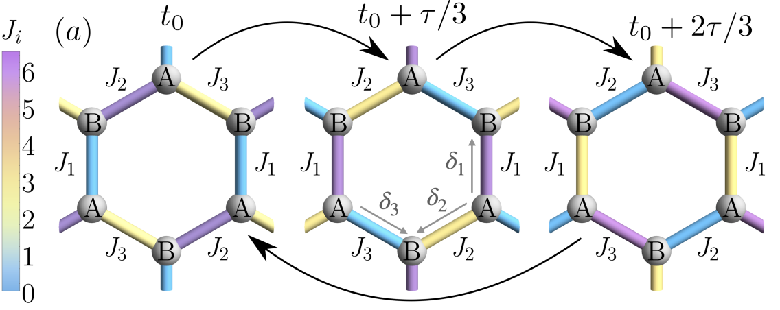
Our work provides numerical evidence that it is indeed possible to stabilize the AFAI phase in the experimentally accessible parameter regimes. However, its indicators are strongly system size dependent. This is because complete localization of bulk states for 2d systems can only be realized for very large system sizes. By considering a Laughlin pump setup we show that the pumped charge over one period of the threaded flux remains quantized even when all bulk states become localized. We work with the continuous driving protocol implemented on a honeycomb lattice as realized in Refs. [16, 17], and add onsite disorder to it. The honeycomb lattice has a 2-sublattice structure which we denote by labels $A$ and $B$ [Fig. 1(a)]. The real-space Hamiltonian is ($\hbar=1$)

where $c_{\bm{i}}^{\dagger}(c^{\vphantom{\dagger}}_{\bm{i}})$ creates (annihilates) a spinless fermion at site $\bm{i}$, $J_{\gamma}(t)=J\exp[F\cos(\Omega t+\phi_{\gamma})]$, with $\phi_{\gamma}=\frac{2\pi}{3}(\gamma-1)$, are the hoppings across three nearest-neighbour bonds $\bm{\beta}_{\bm{i}\gamma}$ at each site $\bm{i}$. If the vector $\bm{i}$ points to a site in the $A\,(B)$-sublattice then $\bm{\beta}_{\bm{i}\gamma}=+(-)\bm{\delta}_{\gamma}$ (for $\gamma=1,2,3$), where $\bm{\delta}_{1}\equiv\quantity(0,a)$, $\bm{\delta}_{2}\equiv\quantity(-\sqrt{3}a/2,-a/2)$, $\bm{\delta}_{3}\equiv\quantity(\sqrt{3}a/2,-a/2)$ [Fig. 1$(a)$], $a$ is the lattice constant, $J$ is the bare hopping amplitude, $\Omega$ is the driving frequency and $F$ is a dimensionless parameter which controls the width of the bulk bands. Henceforth, we set $a=1$, $J=1$ and $F=2$. $V_{\bm{i}}$ is an onsite disorder potential which is sampled from a uniform distribution of width $W$ and zero mean.

According to Floquet’s theorem, such a time-periodic Hamiltonian admits stationary solutions, called Floquet states, of the form $\ket{\psi_{\alpha}(t)}=\exp\quantity(-i\varepsilon_{\alpha}t)\ket{u_{\alpha}(t)}$, where $\varepsilon_{\alpha}$ is the time-independent quasienergy and $\ket{u_{\alpha}(t)}=\ket{u_{\alpha}(t+\tau)}$ is periodic with the time-period $\tau=2\pi/\Omega$ of the drive. Hence, $\ket{u_{\alpha}(t)}$ can be expanded in its harmonics $|u^{(n)}_{\alpha}\rangle=\int_{0}^{\tau}\quantity(\mathrm{d}t/\tau)\exp(in\Omega t)\ket{u_{\alpha}(t)}$, where $n$ is an integer. The Hamiltonian in Eq. (1) can be diagonalized by Fourier transformation [32] to obtain a time-independent eigenvalue problem for the Floquet harmonics $\sum_{\bm{j},m}\tilde{H}^{(n,m)}_{\bm{ij}}u_{\bm{j}\alpha}^{(m)}=\varepsilon_{\alpha}u_{\bm{i}\alpha}^{(n)}$, where $\tilde{H}^{(n,m)}_{\bm{ij}}=\frac{1}{\tau}\int\limits_{0}^{\tau}\mathrm{d}t\,e^{i\quantity(n-m)\Omega t}H_{\bm{ij}}(t)-m\Omega\delta_{nm}\delta_{\bm{ij}}$ is the “Floquet Hamiltonian” [28], $H_{\bm{ij}}(t)$ is the representation of $H(t)$ in a site-localized basis $\{\ket{\bm{i}}\}$, and $u^{(m)}_{\bm{i}\alpha}\equiv\langle\bm{i}|u^{(m)}_{\alpha}\rangle$ is the wavefunction of the $m$-th harmonic of $\ket{u_{\alpha}(t)}$ ($m$ is an integer). Henceforth, the index $\alpha$ shall be restricted to the quasienergies in the first Floquet Brillouin zone (FBZ) $-\Omega/2\leq\varepsilon_{\alpha}<\Omega/2$ [33].

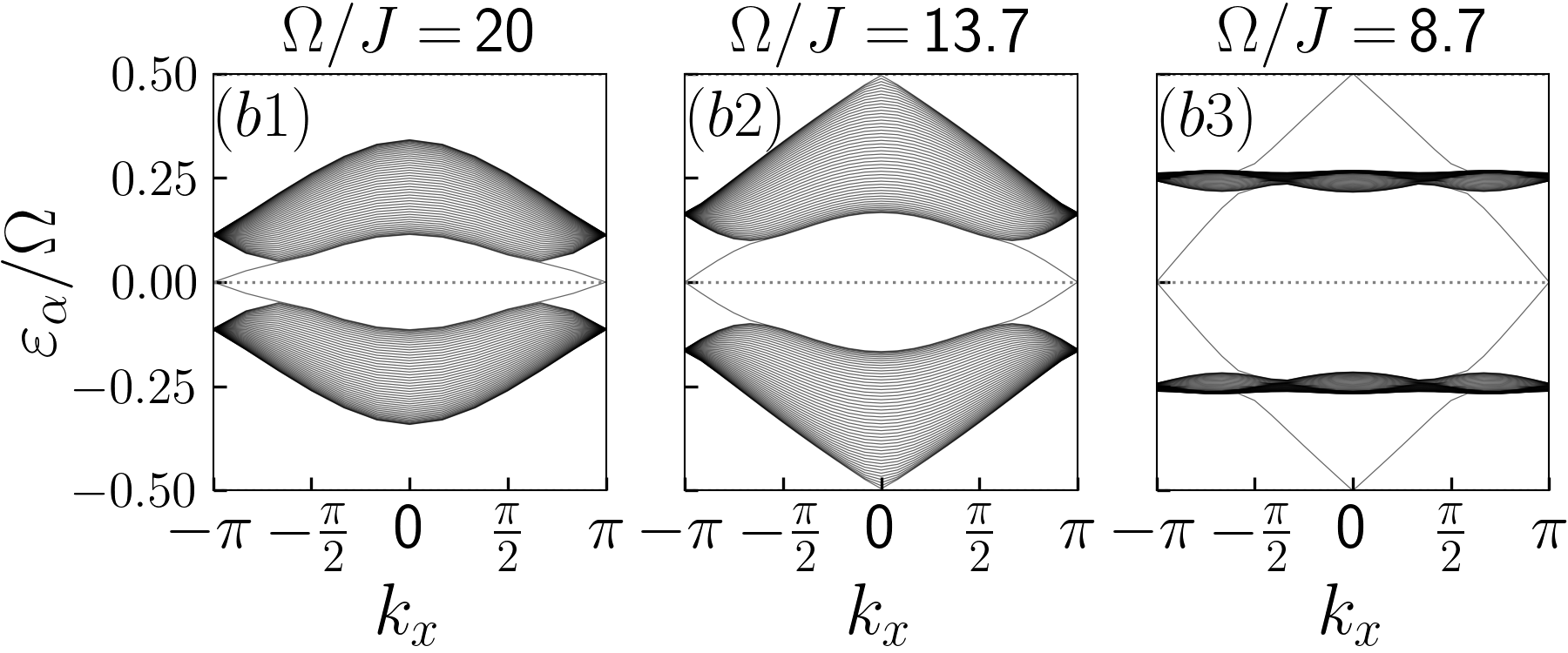
Anomalous Floquet topological insulator (AFTI).$-$We first consider a clean system. In Fig. 1, we plot the dispersion of a semi-infinite strip with zigzag edges for $\Omega/J=20,\,13.7,\,8.7$, and $|m|,|n|\leq N=9$. We define two gaps, the $0(\pi)$-gap having magnitude $\Delta_{0(\pi)}$, respectively, at the center and the edge of the Floquet Brillouin zone for bulk states. For $\Omega/J=20$, the system is a Chern insulator (CI). On decreasing $\Omega/J$, $\Delta_{\pi}$ vanishes at $\Omega/J\approx 13.7$ and the system undergoes a transition from a CI phase to an AFTI phase, akin to that realised in the experiments [16, 17]. The dispersion for a zigzag strip when $\Omega/J$ is tuned across the transition is shown in Fig. 1. In each FBZ, the Chern number of the upper (lower) band $(C^{\pm})$ is given by $C^{\pm}=\mp(\mathcal{W}_{0}-\mathcal{W}_{\pi})$, where $\mathcal{W}_{0(\pi)}$ is an integer topological invariant for the periodically-driven bulk system, called the winding number, which counts the number of chiral edge modes within the gap at quasienergy $0(\Omega/2)$ when the system is defined on a semi-infinite strip. This justifies how the Chern number for all the bulk bands in the anomalous phase can be zero while it hosts robust chiral edge states [27, 28].

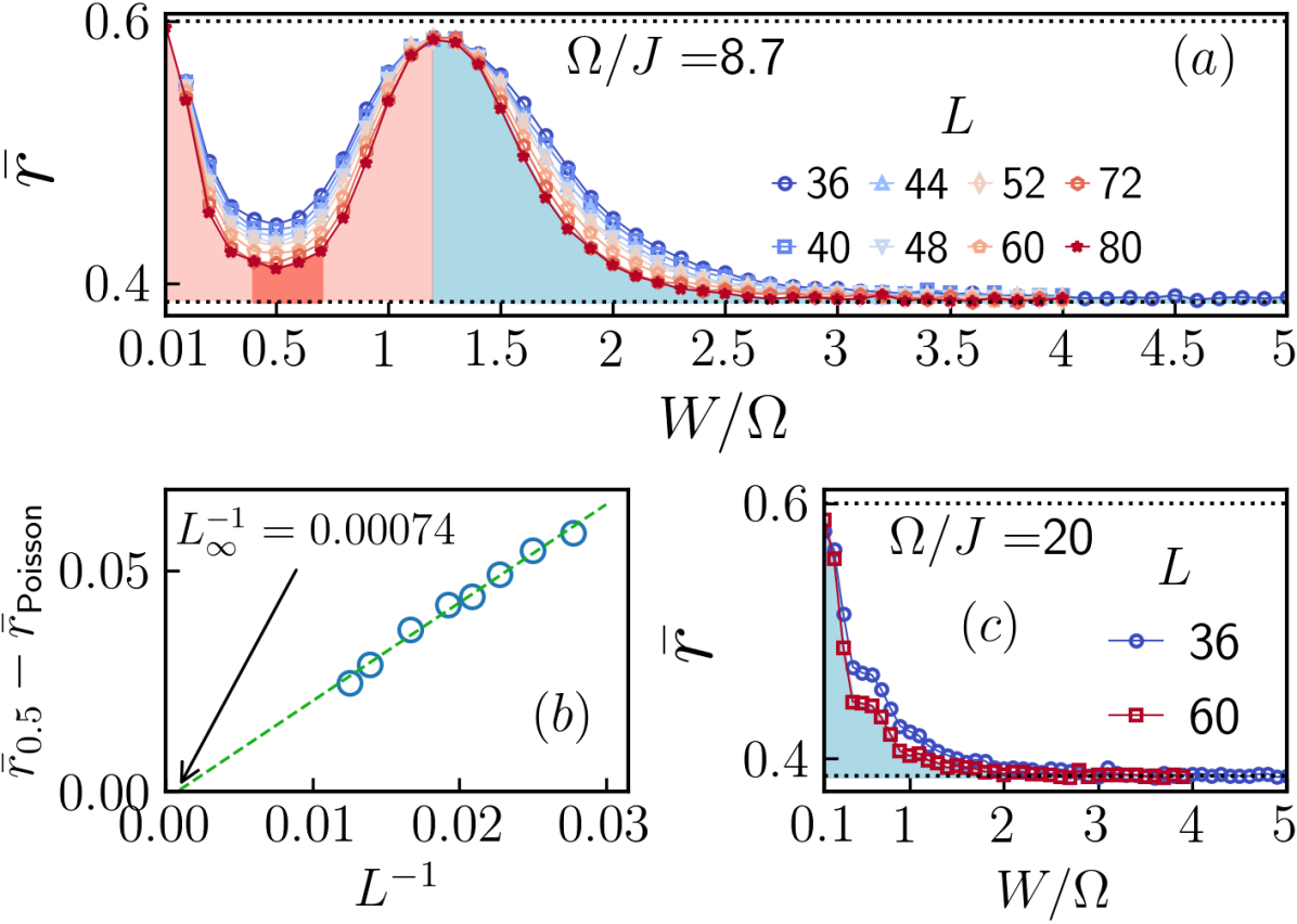
Effect of disorder on the bulk.$-$We focus on two characteristic driving frequencies, $\Omega/J=20$ in the CI phase and $\Omega/J=8.7$ in the AFTI phase, and study the effect of on-site disorder in the bulk. The degree of localisation in a disordered system can be characterised by the level spacing ratio (LSR) $r_{\alpha}$ given by $r_{\alpha}=\min\{s_{\alpha},s_{\alpha-1}\}/\max\{s_{\alpha},s_{\alpha-1}\}$, where $\alpha$ labels the quasienergies within the first FBZ and $s_{\alpha}=\varepsilon_{\alpha+1}-\varepsilon_{\alpha}$ is the spacing between consecutive quasienergy levels. The disorder-averaged LSR distribution is given by $p(r)=\langle\sum_{\alpha}\delta(r-r_{\alpha})\rangle$, where $\langle..\rangle$ denotes disorder averaging. Results from random matrix theory (RMT) suggest that $p(r)$ has a Poissonian form, characterized by the mean LSR ($\bar{r}$) approaching $\bar{r}_{\mbox{\scriptsize Poisson}}=2\ln 2-1\approx 0.39$, if all the states in the system are localized. On the other hand, $p(r)$ in a system without time-reversal invariance, in the thermodynamic limit, for extended states is given by a Wigner-Dyson form corresponding to the Gaussian unitary ensemble (GUE), which is characterized by $\bar{r}_{\mbox{\scriptsize GUE}}=2{\sqrt{3}}/{\pi}-{1}/{2}\approx 0.60$ [34, 35, 30, 36]. Fig. 2$(a)$ and $(c)$ show the behaviour of $\bar{r}$ as a function of disorder strength $W/\Omega$ for $\Omega/J=8.7$ and $20$, respectively. The two-peak structure for $\Omega/J=8.7$, along with its size dependence, indicates the presence of a localized bulk phase around $W/\Omega\approx 0.5$, which is different from the Anderson insulator (AI) phase realized for $W/\Omega\geq 3$. Moreover, the transition from this novel localized phase, which we call the anomalous localized phase, to the AI phase involves a “critical” point [30], at $W/\Omega\approx 1.2$, where $\bar{r}$ attains a maximum value. In the thermodynamic limit, we expect the transition from the anomalous localized phase to the AI phase to be “infinitely sharp” which is supported by the finite size scaling shown in Fig. 2(b).

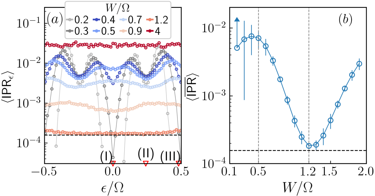
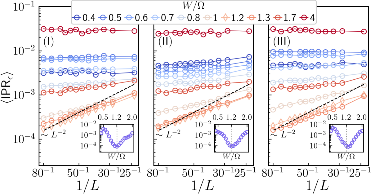
To investigate the localization properties of the anomalous localized phase in more detail, we consider the inverse participation ratio (IPR) for the time-averaged state $|u_{\alpha}^{(0)}\rangle$, defined, for each disorder realization, as $\mbox{IPR}_{\epsilon}\equiv\sum_{\bm{i},\alpha}|\langle\bm{i}|u^{(0)}_{\alpha}\rangle|^{4}\delta(\epsilon-\varepsilon_{\alpha})$, where $\ket{\bm{i}}$ is the site basis state. $\mbox{IPR}_{\epsilon}$ scales as $L^{-2}$ for extended states in $2$-dimensions, where $L$ is the linear dimension. For localized states it becomes independent of system size, for sufficiently large $L$. Fig. 3 (a) shows the disorder averaged IPR, $\langle\mbox{IPR}_{\epsilon}\rangle$ for $\epsilon$ in the first FBZ, for different disorder strengths $W/\Omega$. For $W/\Omega<0.3$, the spectrum has a gap at $\epsilon/\Omega=0$ and $\pm 0.5$, even for the largest system size which could be accessed ($80\times 80$). For $W/\Omega\approx 0.3$, the spectrum becomes gapless for large $L$, but has a gap at lower $L$ values, while for $W\geq 0.4$ the spectrum remains gapless for all the accessed $L$ values. In order to understand the overall behaviour of $\langle\mbox{IPR}_{\epsilon}\rangle$ with changing $W$, we show its mean over $\epsilon$, $\langle\overline{\mbox{IPR}}\rangle$, along with the corresponding standard deviation in Fig. 3 (b). As $W/\Omega$ increases, $\langle\overline{\mbox{IPR}}\rangle$ attains its maximum value near $W/\Omega=0.5$, indicating a maximally localized state on average, and minimum value near $W/\Omega=1.2$, indicating that on average, a maximum number of states are delocalized.

To further support these observations, we show the size dependence of $\langle\mbox{IPR}_{\epsilon}\rangle$ at three characteristic quasienergies chosen at the center $(\mbox{I})$, three-quarters $(\mbox{II})$ and edge $(\mbox{III})$ of the first FBZ in the bottom panel of Fig. 3. These points are indicated by red triangles in Fig. 3 (a). We find that for $0.4\leq W/\Omega\leq 0.7$, $\langle\mbox{IPR}_{\epsilon}\rangle$ remains $L$ independent for $L\geq 60$, across all the three $\epsilon$ slices. Hence, we expect the bulk states at all quasienergies to be localized for this range of $W$ values. Even for lower $L$ values $\langle\mbox{IPR}_{\epsilon}\rangle$ shows almost no scaling at the center and edge of the first FBZ for these values of $W/\Omega$, but shows scaling behaviour for a quasienergy in between them [slice $(\mbox{II})$]. Furthermore, at $W/\Omega\approx 1.2$ we find the emergence of $L^{-2}$ scaling for large $L$, at all the three $\epsilon$-slices, even though the disorder strength is even larger than the bandwidth of the clean system. This confirms the presence of an additional localized phase around $W/\Omega=0.5$ and a localization-delocalization transition around $W/\Omega=1.2$, as indicated by the LSR.

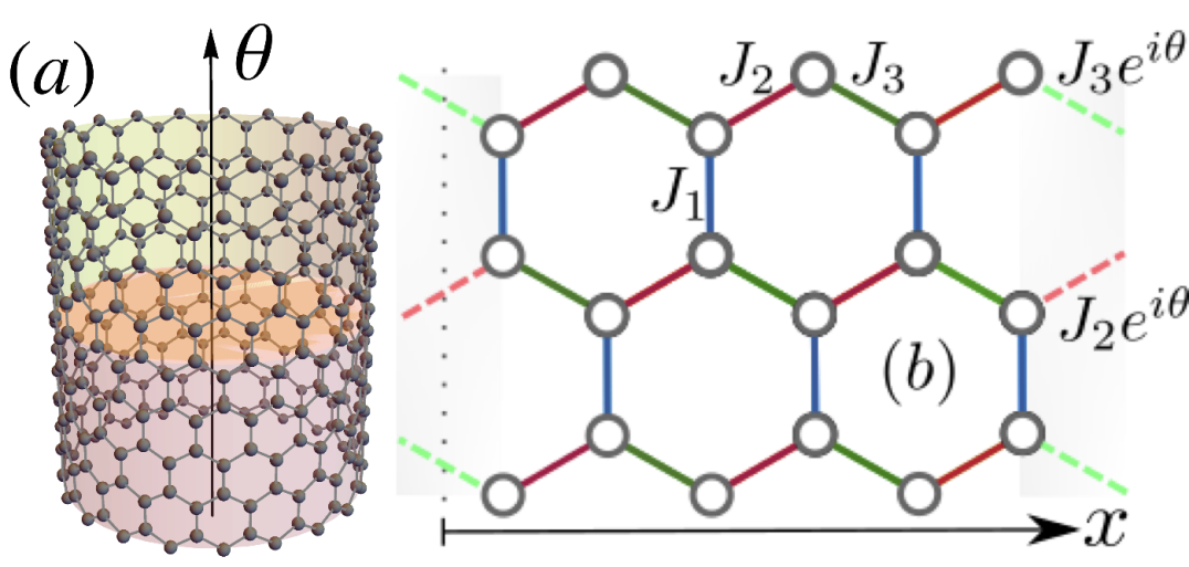
Charge pumping.$-$ The topological properties of the phases can by evaluated by setting up a Laughlin charge pump, where a flux $\theta$ is threaded through the system in a cylindrical geometry [38, 37], as shown in Fig. 4(a). Assuming that the zigzag edge of the cylinder is oriented along the $x$-direction, we choose a gauge such that the nearest-neighbour hopping elements across the bonds which intersect the line $x=0$ acquire an additional phase $\exp(\pm i\theta)$ [30] for hopping to the right (left) [Fig. 4(b)]. The total occupancies in the upper ($\mathcal{U}$) and lower ($\mathcal{L}$) halves of the cylinder are given by $Q_{\mathcal{U}(\mathcal{L})}(\theta)=\sum_{\bm{i}\in\mathcal{U}(\mathcal{L})}Q_{\bm{i}}$, where $Q_{\bm{i}}$ is the occupancy of the site at position $\bm{i}$. The difference between the total particle numbers accumulated in the upper and lower halves of the cylinder is $\delta Q(\theta)=Q_{\mathcal{U}}(\theta)-Q_{\mathcal{L}}(\theta)$ and $P\equiv(\max\{\delta Q(\theta)\}-\min\{\delta Q(\theta)\})/2$ is the pumped charge in one period of the threaded flux $\theta$. In a topologically nontrivial phase, the flux threading is accompanied by a discontinuity of $\delta Q$ as $\theta$ is varied between $[0,2\pi]$ [37].

The site occupancies $Q_{\bm{i}}$ can be expressed in terms of the lesser Floquet Green’s function $G^{<}$ [37, 32, 39]

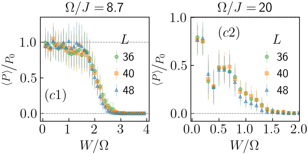
where $f(\omega)\equiv\quantity(1+\exp\quantity(\omega/T))^{-1}$, and $n$ and $p$ are integers. In order to specify an initial state we have introduce a bath at temperature $T$ which is quadratically coupled to the system with a coupling strength $\Gamma$ [32, 40]. However, the experimentally prepared ultracold atomic systems are essentially isolated, so we take the limit $\Gamma\rightarrow 0$ and set $T=0.01$ in Eq. (The anomalous Floquet Anderson insulator in a continuously driven optical lattice). We use $Q_{\bm{i}}$ to calculate the disorder-averaged steady-state pumped charge $\langle P\rangle$, normalized by its reference value $P_{0}$ in the clean system, by tracking the $\theta$ dependence of $\delta Q$ for every disorder realisation. $\langle P\rangle/P_{0}$ has been plotted in Fig. 4 $(c1)$ for $\Omega/J=8.7$ in the anomalous localized phase and in Fig. 4 $(c2)$ for $\Omega/J=20$ in the CI phase. We find that $\langle P\rangle/P_{0}$ remains quantized in the anomalous phase for $W/\Omega<1.2$, while it decreases rapidly with increasing $W/\Omega$ in the CI phase [41]. This means the phase at $\Omega/J=8.7$ supports quantized charge pumping through the edge states while its time-averaged bulk states remain completely localized for $0.4\leq W/\Omega\leq 0.7$. This is the signature of the AFAI phase, as discussed in Ref. [30], which supports one chiral edge mode at each edge of the cylinder, and the two edge modes have opposite chiralities.

Discussion.$-$When all the bulk states are localized then the Chern number at any quasienergy must be zero. However we find that two chiral edge states, each localized at one of edges of the system defined on a cylinder coexist with the localized bulk states [32]. The quasienergies of chiral edge states have a nontrivial flow under flux threading, which gives rise to a quantized pumped charge, as was previously observed in Ref. [30]. The localized bulk states do not flow under threading of flux and hence do not contribute to the charge pumping. It was also shown in Ref. [30] that if one of the edge modes is fully occupied, while the other remains unoccupied, then the net charge flowing across any bond on the occupied edge, per unit time remains quantized, and is equal to the winding number in the bulk when the system has been driven over many cycles. Here we show that the net charge pumped from the bulk to the edges when one quantum of flux is threaded through the cylinder also remains quantized.

Tuning $F$ away from $F=2$, for $\Omega/J=8.7$, increases the dispersion of the bulk bands which has a destabilizing effect on the AFAI phase. We find that the AFAI is stable between $1.9\leq F\leq 2.1$ [32]. Topological edge states have been observed in ultracold atoms by creating a programmable repulsive potential and releasing a localized Bose Einstein condensate near the edge using an optical tweezer. Subsequently, in the clean system, the wave packet propagates along the potential boundary, following its curvature, which is a characteristic for chiral edge states [17]. Such chiral motion at the potential boundary should also be observable in the AFAI, while, in contrast, once the repulsive potential is switched off the initial wave packet should remain localized. For weak disorder, when the system is not in the AFAI phase, sufficiently high energy wave packets, within the first FBZ, will not remain localized, while for strong disorder when the system is in the AI phase, there should be no chiral motion at the edge.

Conclusion.$-$We have studied localization properties and charge pumping in a disordered, circularly driven honeycomb lattice with a continuous driving protocol realized in the experiments [16, 17]. Within the scope of finite size numerics, we found that a new phase emerges at intermediate disorder strength, in which the time-averaged bulk states are fully localized while the system supports quantized charge pumping via edge states, when the system has been evolved over many driving cycles. This is the AFAI phase which was previously predicted in a simplified model [30], which is difficult to realize with ultracold atoms. We also show that the quantized charge pumping in the AFAI phase remains robust at intermediate disorder strength, in contrast to the CI phase. Our approach will also allow us in the future to study the interplay of on-site interactions and strong disorder in the periodically driven system, which can lead to discovery of new phases in hitherto unexplored parameter regimes using Floquet-DMFT [29, 37].

Acknowledgements.$-$This work was supported by the Deutsche Forschungsgemeinschaft (DFG, German Research Foundation) under Project No. 277974659 via Research Unit FOR 2414. J.-H. Z. acknowledges support from the NSFC under Grant No.12247103 and No.12175180, Shaanxi Fundamental Science Research Project for Mathematics and Physics under Grant No. 22JSQ041 and No. 22JSZ005, and the Youth Innovation Team of Shannxi Universities. M.A. also acknowledges support from the Deutsche Forschungsgemeinschaft (DFG) under Germany’s Excellence Strategy – EXC-2111 – 390814868. A.D. thanks Y. Xu for helpful discussions. The authors gratefully acknowledge the Gauss Centre for Supercomputing e.V. (www.gauss-centre.eu) for funding this project by providing computing time through the John von Neumann Institute for Computing (NIC) on the GCS Supercomputer JUWELS at Jülich Supercomputing Centre (JSC). Calculations for this research were also performed on the Goethe-NHR high performance computing cluster. The cluster is managed by the Center for Scientific Computing (CSC) of the Goethe University Frankfurt.

References

- [1] M. S. Rudner and N. H. Lindner, Nat. Rev. Phys. 2, 229 (2020); M. S. Rudner and N. H. Lindner, arXiv:2003.08252.
- [2] A. Eckardt and E. Anisimovas, New J. Phys. 17, 093039 (2015).
- [3] M. Holthaus, J. Phys. B: At. Mol. Opt. Phys. 49, 013001 (2016).
- [4] A. Eckardt, Rev. Mod. Phys. 89, 011004 (2017).
- [5] C. Weitenberg and J. Simonet, Nat. Phys. 17, 1342 (2021).
- [6] W. Hofstetter and T. Qin, J. Phys. B: At. Mol. Opt. Phys. 51, 082001 (2018).
- [7] M. Aidelsburger, S. Nascimbene, N. Goldman, Compt. Rend. Phys. 19, 394 (2018).
- [8] R. Citro and M. Aidelsburger, Nat. Rev. Phys. 5, 87 (2023).
- [9] N. R. Cooper, J. Dalibard, and I. B. Spielman, Rev. Mod. Phys. 91, 015005 (2019).
- [10] T. Ozawa, H. M. Price, A. Amo, N. Goldman, M. Hafezi, L. Lu, M. C. Rechtsman, D. Schuster, J. Simon, O. Zilberberg, and I. Carusotto, Rev. Mod. Phys. 91, 015006 (2019).
- [11] M. Aidelsburger, M. Atala, M. Lohse, J. T. Barreiro, B. Paredes, and I. Bloch, Phys. Rev. Lett. 111, 185301 (2013).
- [12] H. Miyake, G. A. Siviloglou, C. J. Kennedy, W. C. Burton, and W. Ketterle, Phys. Rev. Lett. 111, 185302 (2013).
- [13] M. Aidelsburger, M. Lohse, C. Schweizer, et al., Nat. Phys. 11, 162 (2015).
- [14] G. Jotzu, M. Messer, R. Desbuquois, et al., Nature 515, 237 (2014).
- [15] N. Fläschner, B. S. Rem, M. Tarnowski, D. Vogel, D. S. Lühmann, K. Sengstock, and C. Weitenberg, Science 352, 1091 (2016).
- [16] K. Wintersperger, C. Braun, F. N. Ünal, et al., Nat. Phys. 16, 1058–1063 (2020).
- [17] C. Braun, R. Saint-Jalm, A. Hesse, J. Arceri, I. Bloch and M. Aidelsburger, arXiv:2304.01980.
- [18] J.-H. Zheng, A. Dutta, M. Aidelsburger, and W. Hofstetter, arXiv:2309.07035.
- [19] M. Lohse, C. Schweizer, O. Zilberberg, et al., Nature Phys 12, 350 (2016).
- [20] S. Nakajima, T. Tomita, S. Taie, et al., Nature Phys 12, 296 (2016).
- [21] A. S. Walter, Z. Zhu, M. Gächter, et al., Nat. Phys. (2023).
- [22] M. Rechtsman, J. Zeuner, Y. Plotnik, et al., Nature 496, 196 (2013).
- [23] M. Hafezi, S. Mittal, J. Fan, et al., Nat. Phot. 7, 1001 (2013).
- [24] S. Mittal, V. V. Orre, D. Leykam, Y. D. Chong, and M. Hafezi, Phys. Rev. Lett. 123, 043201 (2019).
- [25] L. Maczewsky, J. Zeuner, S. Nolte, et al., Nat Commun. 8, 13756 (2017).
- [26] S. Mukherjee, A. Spracklen, M. Valiente, et al., Nat. Commun. 8, 13918 (2017).
- [27] T. Kitagawa, E. Berg, M. Rudner, and E. Demler, Phys. Rev. B 82, 235114 (2010).
- [28] M. S. Rudner, N. H. Lindner, E. Berg, and M. Levin, Phys. Rev. X 3, 031005 (2013).
- [29] T. Qin and W. Hofstetter, Phys. Rev. B 96, 075134 (2017).
- [30] P. Titum, E. Berg, M. S. Rudner, G. Refael, and N. H. Lindner, Phys. Rev. X 6, 021013 (2016).
- [31] A. Kundu, M. Rudner, E. Berg, and N. H. Lindner Phys. Rev. B 101, 041403(R) (2020).
- [32] Supplementary material.
- [33] It can be easily verified that for two integers and , if satisfies with the quasienergy , then also satisfies the same eigenvalue problem with quasienergy
- [34] Y. Y. Atas, E. Bogomolny, O. Giraud, and G. Roux, Phys. Rev. Lett. 110, 084101 (2013).
- [35] V. Oganesyan and D. A. Huse, Phys. Rev. B 75, 155111 (2007).
- [36] T. Guhr, A. Müller–Groeling, H. A. Weidenmüller, Phys. Rep. 299, 189 (1999).
- [37] T. Qin, A. Schnell, K. Sengstock, C. Weitenberg, A. Eckardt, and W. Hofstetter Phys. Rev. A 98, 033601 (2018).
- [38] R. B. Laughlin, Phys. Rev. B 23, 5632(R) (1981).
- [39] H. Aoki, N. Tsuji, M. Eckstein, M. Kollar, T. Oka, and P. Werner, Rev. Mod. Phys. 86, 779 (2014).
- [40] T. Qin and W. Hofstetter, Phys. Rev. B 97, 125115 (2018).
- [41] For different disorder realizations, the discontinuities appear at different values. In the numerical implementation, working with a fixed grid makes it impossible to capture the discontinuity for all disorder realizations. This further smears out the transition from the AFAI to the AI phase, and from the CI to AI phase.