The Algorithm for Solving Quantum Linear Systems of Equations With Coherent Superposition and Its Extended Applications

Among the classical algorithms for solving linear equations, the most common one is the Gaussian elimination algorithm. Here, we introduce Gaussian elimination algorithm over binary fields.

We briefly introduce the relevant knowledge of quantum circuits. A circuit composed of multiple quantum gates with certain logic functions is called a quantum circuit. It is applied to a series of operations of a group of qubits and can be used to describe the change of the quantum state in the two-dimensional Hilbert space. Each quantum logic gate can be represented by a unitary matrix.

A single qubit has two quantum ground states $|0\rangle$,$|1\rangle$. If the quantum state $|\varphi\rangle$ is in a state other than the ground state and can be represented linearly by $|0\rangle$ and $|1\rangle$, then the state is called a superposition state $|\varphi\rangle=\alpha|0\rangle+\beta|1\rangle$. The probability amplitudes $\alpha$ and $\beta$ are complex numbers and satisfy $|\alpha|^{2}+|\beta|^{2}=1$.

When given $n$ qubits, the computational basis has $2^{n}$ vectors. After applying a series of quantum gates to the initial state, the original quantum superposition state is changed. Finally, we measure the quantum system and get some $n$-qubit vectors on the computational ground state to obtain our desired results.

In quantum circuits, the unitary operators in the Hilbert space are all reversible, and it may be necessary to use auxiliary qubits to achieve our desired goal. Typically, we can perform some computations, copy the results to an output register using Controlled-NOT (CNOT) gates, and uncompute (performing the same operation backwards) to restore the initial state of the auxiliary qubits. That is, if there is a computational operation $U$, then the uncomputing operation is a hermitian conjugate transpose operator $U^{\dagger}$. Since arbitrary quantum gates can be represented by single-qubit quantum gates and CNOT gates, we focus on these quantum gates. We first show single-qubit quantum gates in Figure 1.

In quantum circuits, multi-qubit gates are often used. Common multi-qubit gates include CNOT gates, Toffoli gates, SWAP gates, and Fredkin gates. The XOR gate in the classical circuit can be implemented by the CNOT gate in the quantum logic gates. Similarly, the Toffoli gate can implement the "AND" operation in quantum computing, and it can also be regarded as a double-controlled CNOT gate. The Fredkin gate can be viewed as a controlled SWAP gate. They are shown in Figure 2.

In an ion-trap quantum computer, CNOT gates can only operate serially. Even though different CNOT gates involve different qubits, they cannot operate in parallel [26]. Therefore, the number of CNOT gates significantly affects the running time of quantum algorithms. When considering the computational complexity of quantum algorithms, we focus on the number of CNOT gates. Since CNOT gates are very critical in quantum computers, in order to calculate the number of CNOT gates in the subsequent article, we decompose a Toffoli gate into single-qubit quantum gates and CNOT gates.

Shende and Markov confirmed [27] that no matter whether the auxiliary system is used or not, at least 6 CNOT gates are needed to implement the Toffoli gate decomposition. A Toffoli gate can be decomposed into six CNOT gates, seven T gates, two H gates, and one S gate. The quantum circuit is as Figure 3.

In [28], seven CNOT gates can be used to implement the decomposition of Fredkin gates. A Fredkin gate can be decomposed into seven CNOT gates, seven T gates, two H gates, and three S gates. The quantum circuit is Figure 4.

Usually, in order to reduce the loss of resources, Toffoli gates are usually used to implement the exchange effect of Fredkin gates, so as to reduce the number of decomposed CNOT gates, such as Algorithm 2 and Algorithm 3 in section 3.

According to Theorem 3, we first translate the classical Gaussian-Jordan elimination Algorithm 4 in the Appendix to the equivalent quantum algorithm, as shown in Algorithm 1.

Brief description of Algorithm 1: If $m<n$, add $(n-m)\times(n+1)$ zero quantum states below the original augmented matrix for Gaussian elimination transformation and a $n\times(n+1)$ all-zero matrix for storing the basic solution system and special solution. First traverse by row, then traverse by column, and use Toffoli gates to find the pivot in each row. If $a_{ij}$ is the first element with 1 in the $i$-th row, mark it as the pivot with a CNOT gate and store it in auxiliary qubits $Pivot_{ij}$; use the $i$-th row to eliminate the row where the element is 1 (except the pivot) in the pivot column. Using $Pivot_{ij}$ as control qubits, exchange the elements of the $i$-th row and the $j$-th row such that the pivot is on the main diagonal. After traversing all the rows and columns, if a column is the pivot column, then the data qubit $a_{jj}$ is 1; otherwise, $a_{jj}$ is 0. Continue to traverse by column, if the $j$-th column is the column where the pivot is located, then use the Toffoli gates to XOR $b_{j}$ to $b_{j+n}$ ($j=1,\cdots,n$), and store it in the special solution; otherwise, use the Toffoli gates to XOR $a_{ij}$ to $a_{(i+n)j}$ ($i,j=1,\cdots,n$) and assign $a_{(j+n)j}$ to 1, then store them in the basic solution system. Then the coefficient before each vector in the basic solution system is obtained to be 0 or 1 by using the Hadamard transformation. By measuring, $x_{j}=b_{j}+k_{1}a_{(j+n)1}+\cdots+k_{n}a_{(j+n)n}$.

We analyze the number of quantum gates needed by quantum Gaussian-Jordan elimination algorithm for solving quantum linear equations. Steps 8-10 need $m(n-1)$ CNOT gates, step 19 needs $n$ CNOT gates, step 24 needs $n$ CNOT gates, the total number of CNOT gates is $mn+2n-m$; steps 8-10 need $\frac{(n-1)mn}{2}$ Toffoli gates, step 12 needs $(m-1)mn$ Toffoli gates, step 13 needs $(m-1)mn(n+1)$ Toffoli gates, step 16 needs $n$ Toffoli gates, step 18 needs $(n-1)n$ Toffoli gates, step 23 needs $n^{2}$ Toffoli gates, the total number of Toffoli gates is $\frac{2m^{2}n^{2}+4m^{2}n-mn^{2}+4n^{2}-5mn}{2}$; step 14 needs $mn(n+1)$ Fredkin gates. Therefore, the number of CNOT gates required is $\mathcal{O}(mn)$; the number of Toffoli gates required is $\mathcal{O}(m^{2}n^{2})$; the number of Fredkin gates required is $\mathcal{O}(mn^{2})$.

In this section, we propose a quantum algorithm that given m n-qubit vectors as input, computes the rank of its span and general solutions. The algorithm can polynomially reduce the number of quantum gates compared with Algorithm 1.

This algorithm needs to add $n\times(n+1)$ zero quantum states as auxiliary qubits above the original quantum state matrix to form a $(m+n)\times(n+1)$ quantum state matrix, which does not change the rank and solution of the original quantum linear system of equations. We can use the original matrix only as the quantum storage register to complete the process of solving the general solution and rank with this quantum algorithm. We use the symbols $tag_{i}$ and $mark_{j}$ (which can be regarded as auxiliary qubits). $tag_{i}$ indicates whether the $i$-th row in the original quantum state matrix is added to the $j$-th row of the all-zero matrix; $mark_{j}$ indicates whether the $j$-th column is the pivot column or the free variable column after adding the zero quantum states as auxiliary qubits.

When $m<n$, the $n\times(n+1)$ matrix added above the original matrix is used to store the quantum state matrix $|U\rangle$ after being transformed into an upper triangle; $(n-m)\times(n+1)$ matrix $O$ below the original matrix is stored in the same register as the original matrix. According to Theorem 1, considering the case where there are solutions, we analyze from the coefficient augmented matrix (ignoring the amplitude here), then the coefficient augmented matrix can be transformed into the form as in formula (1).

When $m\geq n$, only need to add $n\times(n+1)$ quantum states $O$ above the original matrix to store the quantum state matrix $|U\rangle$ transformed into the upper triangle, and its coefficient augmented matrix is transformed into the form as in formula (2).

In the above two formulas, $|a_{ij}\rangle$ in the original matrix corresponds to $|a_{(i+n)j}\rangle$ in the new matrix, $a_{ij}\in\mathbb{F}_{2}$ ; $|b_{i}\rangle$ in the original matrix corresponds to $|b_{(i+n)}\rangle$ in the new matrix, $b_{i}\in\mathbb{F}_{2}$. Initialize $tag_{i}$ and $mark_{j}$, set all $tag_{i}$ to 0 and all $mark_{j}$ to 1. The detailed quantum algorithm is as shown in Algorithm 2.

Brief description of Algorithm 2: add $n\times(n+1)$ zero quantum states above the original matrix, when $m<n$, the $(n-m)\times(n+1)$ zero quantum states need to be added to the original matrix register; when $m\geq n$, there is no need to add the zero quantum states. After traversing all the rows and columns, store the basic solution system and special solution in the original matrix register. The first $n\times n$ qubits store the basic solution system, and $n\times 1$ qubits store the special solution. Use the intermediate variables $tag_{i-n}$ (initialized to 0) and $mark_{j}$ (initialized to 1) for marking. Traverse the elements of the $j$-th column, if $a_{ij}$ ($i=n+1,\cdots,2n$) is the first element with 1 in the $j$-th column, then update the value of $tag_{i-n}$ to 1, the value of $mark_{j}$ to 0, and add the $i$-th row to the $j$-th row to achieve swapping with Toffoli gates; continue to find the element $a_{\ell j}$ ($\ell=1,\cdots,j-1,n+1,\cdots,m+n$) of the $1$-th to the $(j-1)$-th row and the $(n+1)$)-th to the $(m+n)$-th row, $tag_{i-n}$ remains unchanged and is still 0, $mark_{j}$ is still 0 after updating; use the $j$-th row to eliminate the row where the element in the $\ell$-th column is 1 with Toffoli gates. Judge by the updated value of $mark_{j}$, if the value of $mark_{j}$ is 1, then this column is the column where the free variable is located. Add this column to the $j$-th column of the register where the original matrix is located, i.e., the $(n+1)$-th row to the $(2n)$-th row of the $j$-th column of the new matrix, and assign $a_{(j+n)j}$ to 1; if the value of $mark_{j}$ is 0, then this column is the column where the pivot is located, and the $b_{j}$ is the special solution corresponding to the $j$-th row. This special solution is added to the $(n+1)$-th element of the $(n+j)$-th row of the new matrix. The $(n+1)$-th to $(2n)$-th rows of the new matrix correspond to the solutions $x_{1},\cdots,x_{n}$ respectively, and the auxiliary qubits $|k_{h}\rangle$ are subjected to Hadamard transformation, so that the coefficient of the basic solution system is 0 or 1, then add its row to the auxiliary qubits $|solution\rangle$.

Its quantum circuit is as shown in Figure 5:

We analyze the number of quantum gates needed by the quantum algorithm Algorithm 2 for solving the quantum linear equations. Step 10 needs $mn+\frac{n(n-1)}{2}$ CNOT gates, step 14 needs $n$ CNOT gates, step 20 needs $n$ CNOT gates, the total number of CNOT gates is $\frac{2mn+n^{2}+3n}{2}$; step 7 needs $2mn$ Toffoli gates, step 8 needs $mn(n+1)$ Toffoli gates, step 11 needs $mn(n+1)+\frac{n(n-1)(n+1)}{2}$ Toffoli gates, step 13 needs $n(n-1)$ Toffoli gates, step 15 needs $n$ Toffoli gates, step 19 needs $n^{2}$ Toffoli gates, the total number of Toffoli gates is $\frac{4mn^{2}+n^{3}+8mn+4n^{2}-n}{2}$. Therefore, the number of CNOT gates required is $\mathcal{O}(\frac{2mn+n^{2}}{2})$; the number of Toffoli gates required is $\mathcal{O}(\frac{4mn^{2}+n^{3}}{2})$.

More visually, we do not write other registers. when $m<n$, $|A^{\prime}\rangle$ is operated, and $|A^{\prime}\rangle$ will become the following form after Algorithm 2:

where $|\frac{A_{m\times n}}{O_{(n-m)\times n}}\rangle_{n\times n}$ indicates that the all-zero quantum state matrix $|O\rangle_{(n-m)\times n}$ is added below the original matrix $|A\rangle_{m\times n}$, $|\frac{b_{m\times 1}}{O_{(n-m)\times 1}}\rangle_{n\times 1}$ indicates that all-zero vector $|O\rangle_{(n-m)\times 1}$ is added below the constant vector $|b\rangle_{m\times 1}$. $|b^{\prime}\rangle_{n\times 1}$ is a special solution vector, $|\eta\rangle_{n\times n}$ is a basic solution system.

When $m\geq n$, $|A^{\prime\prime}\rangle$ is operated, and $|A^{\prime\prime}\rangle$ will become the following form after Algorithm 2:

where $|\frac{\eta_{n\times n}}{O_{(m-n)\times n}}\rangle_{m\times n}$ indicates that the all-zero quantum state matrix $|O\rangle_{(m-n)\times n}$ is added below the basic solution system $|\eta\rangle_{n\times n}$, $|\frac{b^{\prime}_{n\times 1}}{O_{(m-n)\times 1}}\rangle_{m\times 1}$ indicates that the all-zero vector $|O\rangle_{(m-n)\times 1}$ is added below the special solution vector $|b^{\prime}\rangle_{n\times 1}$. $|U\rangle_{n\times n}$ is an upper triangular quantum state matrix, $|b^{\prime}\rangle_{n\times 1}$ a special solution vector.

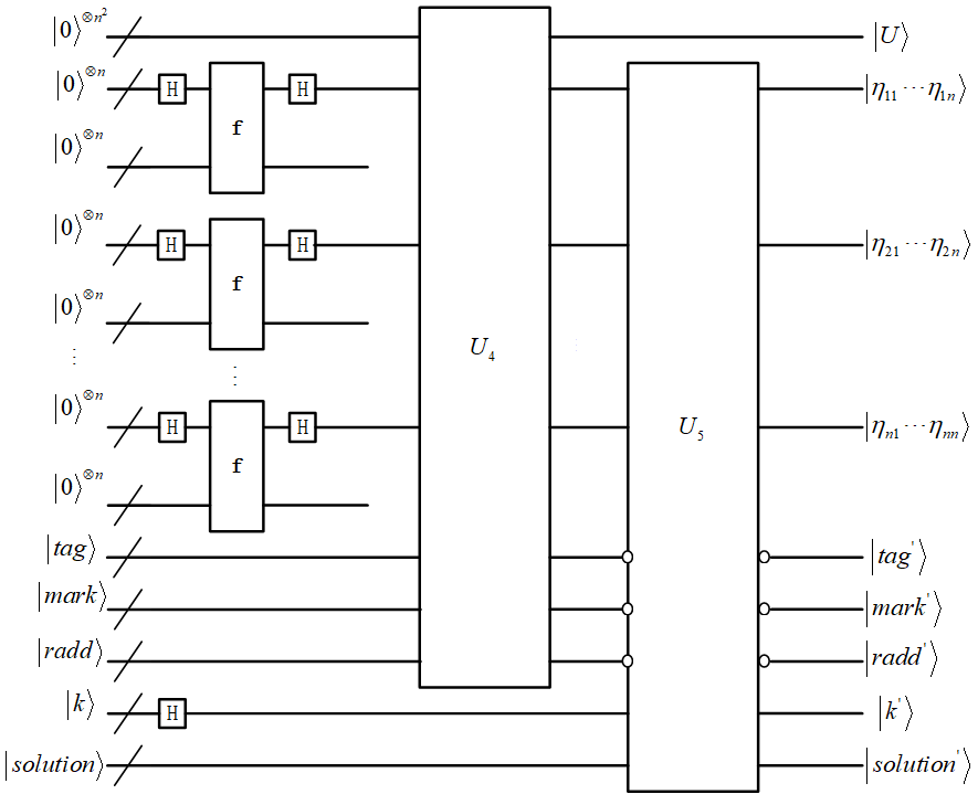
Its universal quantum circuit is as shown in Figure 6.

Note that $|A^{\prime}\rangle_{2n\times(n+1)}$ and $|A^{\prime\prime}\rangle_{(m+n)\times(n+1)}$ are operated respectively when $m<n$ and $m\geq n$. $U_{i}$ means unitary transformation, and the registers are entangled with eacn other after $U_{i}$. "$\circ$" means not to undergo this unitary transformation. In Algorithm 2, for each column, step 7 can be represented by $U_{11}$, step 8 can be represented by $U_{12}$, steps 6-8 can be represented by $U_{1}$, judging whether the row is added and whether the column is the pivot column; steps 9-11 can be represented by $U_{2}$, eliminating the rest elements with 1 in the pivot column; steps 12-15 can be represented by $U_{3}$, judging whether the colum is a free variable column or a pivot column and operating respectively. Steps 5-15 can be represented by $U_{4}$, storing the general solution; steps 16-21 can be represented by $U_{5}$, obtaining the final solution (by last measurement).

This quantum algorithm cannot disentangle the data register containing $|A^{\prime}\rangle$ or $|A^{\prime\prime}\rangle$ with other auxiliary registers since the data register is used as control qubits, and the unitary operation $U_{5}$ is performed. But auxiliary qubits can be saved, and they can be directly used in the circuits of some quantum algorithms for solving linear equations. For example, it can be directly applied to the circuit of parallel Simon’s algorithm (in section 4). However, in the case where we need to obtain the solutions of the quantum linear equations by one measurement at last, the data register can be used as a single input and output, and the data register is disentangled with other auxiliary registers at this time.

We propose another algorithm that uses an auxiliary register as a storage register. This algorithm needs to add $n\times(n+1)$ zero quantum states as auxiliary qubits above and below the original quantum state matrix to form a $(m+2n)\times(n+1)$ quantum state matrix, which does not change the rank and solution of the original quantum linear equations. Similarly, the symbols $tag_{i}$ and $mark_{j}$ are also given. The difference from Algorithm 2 is that we use the $n\times(n+1)$ zero quantum states added below as the storage register for storing the general solution. It can completely disentangle the original quantum coefficient matrix register with other registers and keep data qubits unchanged. According to Theorem 1, considering the case where there are solutions, we analyze from coefficient augmented matrix (ignoring the amplitude), the transformation form is as shown in formula (3), where $|a_{ij}\rangle$ and $|b_{i}\rangle$ of the original matrix correspond to $|a_{(i+n)j}\rangle$ and $|b_{(i+n)}\rangle$, respectively.

References

- [1] Peter W Shor. Algorithms for quantum computation: discrete logarithms and factoring. In Proceedings 35th annual symposium on foundations of computer science, pages 124–134. Ieee, 1994.
- [2] Lov K Grover. A fast quantum mechanical algorithm for database search. In Proceedings of the twenty-eighth annual ACM symposium on Theory of computing, pages 212–219, 1996.
- [3] Lov K Grover. Quantum mechanics helps in searching for a needle in a haystack. Physical review letters, 79(2):325, 1997.
- [4] Hidenori Kuwakado and Masakatu Morii. Quantum distinguisher between the 3-round feistel cipher and the random permutation. In 2010 IEEE International Symposium on Information Theory, pages 2682–2685. IEEE, 2010.
- [5] Marc Kaplan, Gaëtan Leurent, Anthony Leverrier, and María Naya-Plasencia. Breaking symmetric cryptosystems using quantum period finding. In Advances in Cryptology–CRYPTO 2016: 36th Annual International Cryptology Conference, Santa Barbara, CA, USA, August 14-18, 2016, Proceedings, Part II 36, pages 207–237. Springer, 2016.
- [6] Xavier Bonnetain. Quantum key-recovery on full aez. In Selected Areas in Cryptography–SAC 2017: 24th International Conference, Ottawa, ON, Canada, August 16-18, 2017, Revised Selected Papers 24, pages 394–406. Springer, 2018.
- [7] Xavier Bonnetain, Akinori Hosoyamada, María Naya-Plasencia, Yu Sasaki, and André Schrottenloher. Quantum attacks without superposition queries: the offline simon’s algorithm. In Advances in Cryptology–ASIACRYPT 2019: 25th International Conference on the Theory and Application of Cryptology and Information Security, Kobe, Japan, December 8–12, 2019, Proceedings, Part I, pages 552–583. Springer, 2019.
- [8] Daniel R Simon. On the power of quantum computation. SIAM journal on computing, 26(5):1474–1483, 1997.
- [9] Robert Beals, Harry Buhrman, Richard Cleve, Michele Mosca, and Ronald De Wolf. Quantum lower bounds by polynomials. Journal of the ACM (JACM), 48(4):778–797, 2001.
- [10] Hidenori Kuwakado and Masakatu Morii. Security on the quantum-type even-mansour cipher. In 2012 International Symposium on Information Theory and its Applications, pages 312–316. IEEE, 2012.
- [11] THOMAS SANTOLI and CHRISTIAN SCHAFFNER. Using simon’s algorithm to attack symmetric-key cryptographic primitives. Quantum Information and Computation, 17(1&2):0065–0078, 2017.
- [12] Xavier Bonnetain, María Naya-Plasencia, and André Schrottenloher. On quantum slide attacks. In Selected Areas in Cryptography–SAC 2019: 26th International Conference, Waterloo, ON, Canada, August 12–16, 2019, Revised Selected Papers, pages 492–519. Springer, 2020.
- [13] Gregor Leander and Alexander May. Grover meets simon–quantumly attacking the fx-construction. In Advances in Cryptology–ASIACRYPT 2017: 23rd International Conference on the Theory and Applications of Cryptology and Information Security, Hong Kong, China, December 3-7, 2017, Proceedings, Part II 23, pages 161–178. Springer, 2017.
- [14] Aram W Harrow, Avinatan Hassidim, and Seth Lloyd. Quantum algorithm for linear systems of equations. Physical review letters, 103(15):150502, 2009.
- [15] Dominic W Berry, Andrew M Childs, Richard Cleve, Robin Kothari, and Rolando D Somma. Exponential improvement in precision for simulating sparse hamiltonians. In Proceedings of the forty-sixth annual ACM symposium on Theory of computing, pages 283–292, 2014.
- [16] Andrew M Childs, Robin Kothari, and Rolando D Somma. Quantum algorithm for systems of linear equations with exponentially improved dependence on precision. SIAM Journal on Computing, 46(6):1920–1950, 2017.
- [17] Leonard Wossnig, Zhikuan Zhao, and Anupam Prakash. Quantum linear system algorithm for dense matrices. Physical review letters, 120(5):050502, 2018.
- [18] Iordanis Kerenidis and Anupam Prakash. Quantum recommendation systems. In Christos H. Papadimitriou, editor, 8th Innovations in Theoretical Computer Science Conference, ITCS 2017, January 9-11, 2017, Berkeley, CA, USA, volume 67 of LIPIcs, pages 49:1–49:21. Schloss Dagstuhl - Leibniz-Zentrum für Informatik, 2017.
- [19] Yiğit Subaşı, Rolando D Somma, and Davide Orsucci. Quantum algorithms for systems of linear equations inspired by adiabatic quantum computing. Physical review letters, 122(6):060504, 2019.
- [20] Simone Perriello, Alessandro Barenghi, and Gerardo Pelosi. A complete quantum circuit to solve the information set decoding problem. In 2021 IEEE International Conference on Quantum Computing and Engineering (QCE), pages 366–377. IEEE, 2021.
- [21] Andre Esser, Sergi Ramos-Calderer, Emanuele Bellini, José I. Latorre, and Marc Manzano. An optimized quantum implementation of ISD on scalable quantum resources. CoRR, abs/2112.06157, 2021.
- [22] Charles H Bennett and Gilles Brassard. Quantum cryptography: Public key distribution and coin tossing. Theoretical Computer Science, 560:7–11, 2014.
- [23] Marcos Curty and David J Santos. Quantum authentication of classical messages. Physical Review A, 64(6):062309, 2001.
- [24] Chuan Wang, Fu-Guo Deng, Yan-Song Li, Xiao-Shu Liu, and Gui Lu Long. Quantum secure direct communication with high-dimension quantum superdense coding. Physical Review A, 71(4):044305, 2005.
- [25] Xavier Bonnetain and Samuel Jaques. Quantum period finding against symmetric primitives in practice. IACR Transactions on Cryptographic Hardware and Embedded Systems, 2022(1):1–27, 2021.
- [26] Li Yang and Rui-Rui Zhou. On the post-quantum security of encrypted key exchange protocols. arXiv preprint arXiv:1305.5640, 2013.
- [27] Vivek V Shende and Igor L Markov. On the cnot-cost of toffoli gates. Quantum Information & Computation, 9(5):461–486, 2009.
- [28] Amit Saha and Om Khanna. Intermediate-qudit assisted improved quantum algorithm for string matching with an advanced decomposition of fredkin gate. CoRR, abs/2304.03050, 2023.
- [29] Michael A Nielsen and Isaac L Chuang. Quantum computation and quantum information. Cambridge university press, 2010.
- [30] Gilles Brassard, Peter Hoyer, Michele Mosca, and Alain Tapp. Quantum amplitude amplification and estimation. Contemporary Mathematics, 305:53–74, 2002.
- [31] Ye Wang, Mark Um, Junhua Zhang, Shuoming An, Ming Lyu, Jing-Ning Zhang, L-M Duan, Dahyun Yum, and Kihwan Kim. Single-qubit quantum memory exceeding ten-minute coherence time. Nature Photonics, 11(10):646–650, 2017.
- [32] Biyao Yang and Li Yang. Effect on ion-trap quantum computers from the quantum nature of the driving field. Science China Information Sciences, 63:1–15, 2020.
- [33] Joe Kilian and Phillip Rogaway. How to protect des against exhaustive key search. In Advances in Cryptology—CRYPTO’96: 16th Annual International Cryptology Conference Santa Barbara, California, USA August 18–22, 1996 Proceedings 16, pages 252–267. Springer, 1996.
- [34] Julia Borghoff, Anne Canteaut, Tim Güneysu, Elif Bilge Kavun, Miroslav Knezevic, Lars R Knudsen, Gregor Leander, Ventzislav Nikov, Christof Paar, Christian Rechberger, et al. Prince–a low-latency block cipher for pervasive computing applications. In Advances in Cryptology–ASIACRYPT 2012: 18th International Conference on the Theory and Application of Cryptology and Information Security, Beijing, China, December 2-6, 2012. Proceedings 18, pages 208–225. Springer, 2012.
- [35] Martin R Albrecht, Benedikt Driessen, Elif Bilge Kavun, Gregor Leander, Christof Paar, and Tolga Yalçın. Block ciphers–focus on the linear layer (feat. pride). In Advances in Cryptology–CRYPTO 2014: 34th Annual Cryptology Conference, Santa Barbara, CA, USA, August 17-21, 2014, Proceedings, Part I 34, pages 57–76. Springer, 2014.
Appendix
Gaussian-Jordan Elimination over Binary Fields
We first give a lemma about the relationship between the rank of the matrix and the number of the basic solution vectors, so as to understand the Gaussian-Jordan elimination algorithm over binary fields.
Lemma 3.
(Rank of matrix over binary fields) Given a matrix over binary fields, then its rank equals the number of unknown variables minus the number of the basic solution vectors.
Proof.
Let be the rank of , and be the number of basic solution vectors.
equals the dimension of the column space of , i.e., the maximum number of linearly independent column vectors of . The matrix has columns in total, and the number of free vector columns is , so the rank of is equal to , the number of basic solution vectors (consists of free vector columns) is . Therefore, the rank of the matrix is equal to the number of unknown variables minus the number of basic solution vectors , i.e., . ∎
According to Lemma 3, we can know that given a matrix over binary fields, when , the number of basis vectors of the solution is , then its coefficient augmented matrix must be transformed into the following form through Gaussian-Jordan elimination method and row-column transformation:
The -th to -th columns are the columns where the free variables are located, then the basic solution system of the linear equations is:
The special solution of the linear equations is . We can obtain the general solution is , where .
Since the above form has undergone a column transformation, the order of the variable vectors corresponding to the special solution and the basic solution system is not sequential. When the general solution is given, the order of the variable vectors still needs to be adjusted. Algorithm 4 gives the method for solving the general solution of the linear equations without column transformation, and the order of the variable vectors does not change at this time.
The row echelon matrix is the middle matrix form of the elimination step in the Gaussian elimination method, which is also a critical step. The row reduced form matrix is the final matrix form after the Gauss-Jordan elimination operation. Based on the two forms, after performing elementary transformations on augmented matrices, we give a Gaussian-Jordan elimination algorithm 4 for the general solutions of linear equations over binary fields.
Brief description of Algorithm 4: Initialization the list, including Pivot, , and base solution system list. If , use the all-zero elements to complement the list into a matrix; if , the matrix remains unchanged. First traverse by row and then traverse by column, if is the first element with 1 in the -th row, mark it as the pivot and store the column index in the list Pivot. Use the -th row to eliminate the row where the element 1 is located in the -th column. Swap the -th row and the -th row so that all pivots are on the main diagonal. After traversing all the rows and columns, at this time, Pivot stores the index of the columns where all the pivots are located in row order. Afterwards, continue to traverse by column, if is in the list Pivot, it means that there is a pivot element in this column, then traverse by row, find the pivot, swap the -th row and the -th row such that the pivot is on the main diagonal, and store the special solution corresponding to in the list at this time, otherwise add zero to the list . If is not in the list Pivot, add the elements in this column to the list in reverse order, and assign the -th element in to 1. Finally, we can obtain the general solution , and the rank is the length of the list Pivot.
A Proof of Theorem 4
Given a lemma in [5], as follows:
Lemma 4.
For , consider function , Where, . For , satisfy