The spectral radius of -connected graphs with given diameter
Abstract
Let be a graph with adjacency matrix and degree diagonal matrix . In 2017, Nikiforov defined the matrix for any real . The largest eigenvalue of is called the spectral radius or the -index of . Let be the set of -connected graphs with order and diameter . In this paper, we determine the graphs with maximum spectral radius among all graphs in for any , where and . We generalizes the results of adjacency matrix in [P. Huang, W.C. Shiu, P.K. Sun, Linear Algebra Appl., 2016, Theorem 3.6] and the results of signless Laplacian matrix in [P. Huang, J.X. Li, W.C. Shiu, Linear Algebra Appl., 2021, Theorem 3.4]. Key Words: spectral radius; -connected; diameter AMS Subject Classification (2020): 05C50
1 Introduction
All graphs considered here are simple. Let be a graph with vertex set and edge set . The order of is and the size of is , where and . The neighbor set of a vertex in is denoted by , the degree of the vertex in is denoted by , where . The minimum degree and the maximum degree of are denoted by and , respectively. The distance between two distinct vertices of a connected graph is the length of the shortest path connecting them. The diameter of is the maximum distance among all distinct vertices pairs of . For a subset , let be the subgraph induced by and . A graph is -connected if is connected for any subset with . The sequential join of graphs , is the graph formed by taking one copy of each graph and adding additional edges from each vertex of to all vertices of , for . A path and a complete graph of order are denoted by and , respectively. Unless otherwise stated, we use the standard notations and terminologies in [2, 23].
The spectral radius of a graph is the largest eigenvalue of , where is a responding graph matrix defined in a prescribed way, such as adjacency matrix, (signless) Laplacian matrix and others. The adjacency matrix of a graph with order is an 0-1 matrix, denoted by , where if , and otherwise. The degree diagonal matrix of is . The Laplacian matrix of a graph is , and the signless Laplacian matrix of is . In 2017, Nikiforov [19] defined the matrix of a graph as for any real , which can underpin a unified theory of and . The spectral radius of a graph is denoted as . Based on the well-known Perron-Frobenius theorem, there exists a positive eigenvector corresponding to , also called the Perron vector of . For a vertex , the eigenequation of corresponding to is written as
| (1) |
Moreover, we have
| (2) |
By Rayleigh Quotient, we have
| (3) |
The Brualdi-Solheid problem, which was first presented in 1986 by Brualdi and Solheid in article [3], is a well-known question about finding a tight bound for the spectral radius in a set of graphs and characterizing the extremal graphs. Many recent results on this problem for various kinds of graphs and their adjacency spectral radius have been obtained, we refer to articles [1, 7, 8, 24, 29], some monographs [22, 23] and the references therein. The results of the Brualdi-Solheid problem about the signless Laplacian spectral radius and spectral radius, we refer to articles [10, 11, 15, 18, 28] and [4, 9, 12, 16, 21, 30], respectively. Further, other results for the spectral radius of digraph can be refered to [17, 25, 26] and the references therein. Recently, the spectral extremal problem of adjacency matrix and matrix has also attracted lots of attention, some results can be found in articles [5, 6] and the references therein.
Let be the set of -connected graphs of order with given diameter . Huang, Shiu, Sun [14] and Huang, Li, Shiu [13] solved the Brualdi-Solheid problem in for adjacency spectral radius and signless Laplacian spectral radius, respectively. Their conclusions are as follows.
Theorem 1.1 ([13, 14]).
For and , the graph attains the maximum signless Laplacian spectral radius in , where for , and .
Furthermore, Huang, Li and Shiu [13] believed that the results of Theorem 1.1 also hold for spectral radius in with . For , it is obvious that is the unique graph with the maximum spectral radius. For and , Xue et al. [27] characterized that is the unique graph with the maximum spectral radius, where is the graph obtained from by connecting its all vertices to an end vertex of and an end vertex of . In this paper, we confirm Huang, Li and Shiu’s conjecture for all and . Our conclusion is as follows.
Theorem 1.2.
For and , the graph attains the maximum spectral radius in , where for each , . Further,
2 Preliminaries
In this section, we present some preliminary results, which will be used in Section 3.
A graph is called diameter critical if its diameter decreases with any addition of an edge. The structure of a diameter critical -connected graph was characterized by Ore [20] in 1968.
Lemma 2.1 ([20]).
Let be a graph in . If is a diameter critical graph, then , where for each .
Following that, we present several results on the spectral radius. In this paper, the vertices and of are said to be equivalent, if there exists an automorphism : such that .
Lemma 2.2 ([19]).
Let . Then .
Lemma 2.3 ([19]).
Let be a connected graph and be a proper subgraph of . Then for .
Lemma 2.4 ([19]).
Let be a connected graph. Let and be two equivalent vertices in . If is the positive eigenvector of corresponding to , then for .
Lemma 2.5 ([19]).
Let be a graph with maximum degree . If , then
If is connected, then equality holds if and only if . In particular,
Lemma 2.6.
Lemma 2.7 ([27]).
Let be a connected graph and be a positive eigenvector of corresponding to . For two distinct vertices , of , suppose . Let . If and , then for .
In order to prove our main results, we generalize Lemma 2.7, our conclusion is shown in Lemma 2.8. In addition, we characterize the spectral radius about the sequential join of three complete graphs , , and , the results are shown in Lemma 2.9.
Lemma 2.8.
Let be a connected graph and be a positive eigenvector of corresponding to . Let and be two disjoint subsets of that satisfy . For each pair of vertices , resp. , are equivalent in , then resp. . Suppose . Let be a graph from by deleting all edges between and and adding all edges between and . If , then .
Proof.
Lemma 2.9.
Let . Then is the largest root of , where
In Particular, we have the following two results.
-
(i)
If , then , where
-
(ii)
If , then .
Proof.
Note that all vertices in , all vertices in and all vertices in are equivalent, respectively. Let be the Perron vector corresponding to , where for each . By Equation (1), we have
| (4) |
Let be the determinant of the coefficient matrix of the Equation (4). Notice that , by using the theory of solving homogeneous linear equations, then is the largest root of , where
-
(i)
If , then the vertices in are equivalent in , that is . similarly we have
Similarly, according to the theory of solving homogeneous linear equations, by direct calculation, we have , where
-
(ii)
If , by direct calculation, then
These complete the proof. ∎
Lemma 2.10.
Let . Then , where . In Particular, if , then .
3 Proof of Theorem 1.2
Let be the graph with the maximum spectral radius among all graphs in . We call the graph is maximal in .
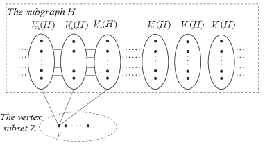
According to Lemmas 2.1 and 2.3, the maximal graph must be diameter critical. Since adding edges increases the spectral radius. We have , where and for each , as shown in Figure 1. The vertices sets of the subgraph in are simply denoted as for each . Therefore, is a partition of .

Note that any two distinct vertices in (resp. ) are equivalent. Let be the Perron vector corresponding to . Then we have .

Let be a subgraph of with vertex set . Let , where , , as shown in Figure 2. Thus is a partition of , where , , and for each . Similarly, is a partition of . It is possible that for some , for instance .
Let be the set of all graphs of order , in which each graph is isomorphic to , where , and there exists only one such that and for each . Obviously, .
Next, we keep the notations defined in the preceding section unless otherwise stated and prove several Lemmas.
Lemma 3.1.
Let be a maximal graph in . If and , then .
Proof.
For and , it is obvious that . Next we consider and .
By contradiction, we suppose , then there exists at least two ,…, such that and for each , which also implies that .
For and , if , then and . Let be a graph obtained from by deleting all edges between and and adding all edges between and . Without loss of generality, we assume . Since , by using Lemma 2.7, we have . Note that , which contradicts the assumption that is the maximal graph in . Thus .
Next we consider and . Let be three largest values in the set of the graph , where , and are pairwise distinct. Next we consider the following two cases:
-
Case 1.
or .
For any a vertex , let be three elements of the vertex partition set of , whose vertices are adjacent to . It is possible that . Because , without loss of generality, we assume , and .
-
Step 1.
Let be a graph obtained from by deleting all edges between and , , , respectively, and adding all edges between and , , , respectively.
For or , the graph and the graph ( or ) is shown in Figure 3 (), (), respectively. In Figure 3 (), we denote the edge-shifting operation from the graph to the graph ( or ) as ( or ), where the thick dashed lines are the deleted edges in the graph and the thick solid lines are the added edges in the graph . In Figures 39, take Figure 3 () as an example, we just show the edge-shifting operations between the corresponding two graphs.
If or , by using Equations (2) and (3), then
If or , by symmetry, we can suppose . By using Equations (2) and (3), then we have
Therefore, .
(a) The graph ( or ). 
(b) The graph ( or ). 
(c) The edge-shifting operations from to ( or ). Figure 3: ( or ). -
Step 2.
Let be a vertex of and .
If or , let be three elements of the vertex partition set of , whose vertices are adjacent to . According to our assumption, , thus without loss of generality, we assume , , . Next we do the same operation as Step 1. and obtain a graph from by deleting all edges between and , , , respectively, and adding all edges between and , , , respectively. ThenIf or , by symmetry, we suppose . By using Equations (2) and (3), then we have
Repeat this step until all of the vertices in have been chosen. Thus in the final graph, denoted by , all vertices in are adjacent to , and , and .
In order to ensure that the maximal graph after the edge-shifting operation is still a diameter critical graph, and prove that our conclusions hold, we do the Step 3.
-
Step 3.
Let be the graph obtained from by adding some edges so that is a clique. Then .
If , then our results hold. Next we consider the following two cases.-
Case 1.1.

Figure 4: . .
Let be the graph obtained from by deleting all edges between and , all edges between and , and adding all edges between and , all edges between and , as shown in Figure 4.
If , then
If , then
Then , and . This contradicts that is the maximal graph in . Thus the maximal graph .
-
Case 1.2.

Figure 5: . .
Let be the graph obtained from by deleting all edges between and , all edges between and , all edges between and , all edges between and , and adding all edges between and , all edges between and , all edges between and , all edges between and , as shown in Figure 5.If , then
If , then
Then and . This contradicts that is the maximal graph in . Thus the maximal graph .
-
Case 1.1.
-
Step 1.
-
Case 2.
or .
Since , by using Proposition 36. in [19] and Lemma 2.3, then , that is . Because of symmetry, we have . Thus, or , where . Without loss of generality, we assume , where . Next we consider two cases: first, , second, . The case of can be converted to the case that and by using some edge-shifting operations.-

Figure 6: . 
Figure 7: . 
Figure 8: . 
Figure 9: . 
Figure 10: . 
Figure 11: . -
Case 2.1.
.
Let be the three largest components of corresponding to all vertices of , , (, and are pairwise distinct), respectively. We follow all steps as Case 1., then we can obtain the graphs like , , , , or , such that , where and are in . Then we obtain a same contradiction like Case 1. that is a maximal graph in and . -
Case 2.2.
and .
Let be a graph obtained from by deleting all edges between and , , respectively, and adding all edges between and , , respectively, as shown in Figure 6. Then there is no edge between and . By using Lemma 2.8, then . The following discussion also applies to the case that one of , is not an empty set.First, we choose one vertex from . Let be a graph obtained from by deleting all edges between and , all edges between and , and adding all edges between and , and the edge , see Figure 7. By using Lemma 2.8, we have .
Second, let be a graph obtained from by adding all edges between and , as shown in Figure 8. By using Lemma 2.3, we have .
Third, if , then we may follow the proof of Case 1., otherwise, if , let be a graph obtained from by deleting all edges between and , and adding all edges between and , as shown in Figure 9. By using Lemma 2.8, we have . Next, we may follow the proof of Case 1. and get a contraction. Thus the maximal graph .
-
Case 2.3.
and ().
First, we keep all edges between and , keep all edges between and . Next we delete all edges between and and add all edges between and .Second, let be the largest component of . Then we repeat the similar operations of Step 1.–Step 3. in Case 1. and obtain a graph with , as shown in Figure 10. Let be a graph obtained from by deleting all edges between and , all edges between and , and adding all edges between and , all edges between and , as shown in Figure 11. Then by using Lemma 2.3, we have . Note that the graph satisfys , and in the graph , one of and and . It belongs to Case 2.2.
-
These complete the proof of Lemma 3.1. ∎

Lemma 3.2.
Let , where , , for each , as shown in Figure 12. Let be the Perron vector of the graph corresponding to , where for each . If , , and . Then
-
(i)
and .
-
(ii)
.
-
(iii)
and for each , where .
Proof.
We keep all notations above unless otherwise stated. Let . Since , by Lemmas 2.2 and 2.3, then . By Equation (1), we have , then for any .
(i) and .
In terms of symmetry, we just consider . It is similar for . Next we are going to consider the following two cases:
Case 1. .
By the eigenequations of , we have the following recurrence equations:
| (5) |
Let be a sequence of numbers satisfying the above recursive formula. Thus its characteristic equation is
| (6) |
Notice that , then , thus Equation (6) has two different real roots and such that
It is clear that . Since , if , then the Equation (6) is equal to . By Lemmas 2.3, 2.9(i), for , we have , if , then the Equation 6 is equal to , that is . Therefore, we have . By the theory of linear recurrence equation about the sequence, there exist and such that , . The boundary conditions are as follows:
Then
That is,
Thus
where
Since , and for any , then .
By using Lemma 2.9(i), we have . Then for , then we have Thus , for any .
Let , and .
Notice that , then we have
Thus we have , for each when . By symmetry, we have , for each where .
Case 2. .
It is clear that holds for and . Next we are going to proof that holds for , that is . By the eigenequations of corresponding to and , we have
Then we have
Thus Let , . Therefore, in order to prove , we only need to prove . Let . By direct calculation, we have
Note that is a fuction of , so has solutions if and only if . Note that . By direct calculation, it is easy to prove that holds for and .
Thus in order to prove , we need to prove that is greater than the maximum solution of , that is . Notice that , then we need to prove that , which is equivalent to prove . Let . By direct calculate, we have holds for each . Thus, if k is greater than the maximum solution of , then . By direct calculation, we have the maximum solution of is for each . Thus holds for each and each . Thus . Then .
Thus we have , for each when . By symmetry, we have , for each when .
These complete the proof of (i) in this Lamma 3.2. Next we are going to prove .
(ii) .
By the eigenequation corresponding to , that is
Note that , and . Then we have
Thus we have . These complete the proof of the first and second results (i) and (ii) in this Lamma 3.2.
(iii) and for each , where .
By the eigenequations of , we have
Since and , then
| (7) |
Notice that , by the eigenequations corresponding to , , these are
Thus . Since , then , by Equation (7), we have and , for each .
These complete the proof of this Lemma 3.2. ∎
In the following, we use all the notations in Lemma 3.2 unless otherwise stated.
Lemma 3.3.
Let be a maximal graph in . Suppose , then .
Proof.
By Lemma 3.2, we have , so , . Recall that . Let be a graph obtained from the maximal graph by deleting all edges between and and adding all edges between and . If , then by Lemma 2.8, we have . Thus this contradicts that is the maximal graph in . Thus . Similarly, we have . Next we prove .
Suppose . We select one vertex of . Since , then we denote the two vertices in , as , , respectively. Let be a graph obtained from by deleting all edges between and , all edges between and , edge , and adding edge , all edges between and , all edges between and . Obviously, . Then
Thus if , then holds.
Next we obtain the graph by using a different edge-shifting operation. Let be the graph obtained from by deleting all edges between and , all edges between and and adding all edges between and , all edges between and . Then we have
Thus if and , then holds. Through gradual recursion, let be the graph obtained from by deleting all edges between and , all edges between and and adding all edges between and , all edges between and , for . Thus we have if , then , ,, . There is a contradiction that in the maximal graph . Thus .
Assume for , and we now prove . Let be a graph obtained from by deleting all edges between and , all edges between and and adding all edges between and , all edges between and . Then
Since , we have , for each . These complete the proof. ∎
Now we have all the ingredients to present our proof of Theorem 1.2.
Proof of Theorem 1.2.
In this proof, we use the notations in Lemma 3.2 unless otherwise stated. Let , where , , , , as shown in Figure 12. By Lemma 3.1, the result hold when or . Thus we only consider the case in the following.
In order to prove a contradiction, we suppose . Let be a graph obtained from by deleting all the edges between and and the edges between and , then adding all the edges between and and the edges between and . Evidently, . Note that by Lemma 3.2 and . Then from Equation 2, we have
Thus , which contradicts the fact that is the maximal graph in . Thus we have .
References
- [1] A. Berman, X-D. Zhang. On the spectral radius of graphs with cut vertices, J. Combin. Theory Ser. B., 83(2) (2001) 233–240.
- [2] J.A. Bondy, U.S.R. Murty. Graph Theory, Springer, New York, 2008.
- [3] R.A. Brualdi, E.S. Solheid. On the spectral radius of complementary acyclic matrices of zeros and ones, SIAM J. Algebraic Discrete Methods, 7(2) (1986) 265–272.
- [4] C.H. Chen, J.R. Peng, T.Y. Chen. The -spectral radius of complements of bicyclic and tricylic graphs with vertices, Spec. Matrices, 10 (2022) 55–66.
- [5] S. Cioabă, D.N. Desai, M. Tait. The spectral radius of graphs with no odd wheels, European J. Combin., 99 (2022) 103420.
- [6] S. Cioabă, L.H. Feng, M. Tait, X-D. Zhang. The maximum spectral radius of graphs without friendship subgraphs, Electron. J. Combin., 27 (2020) Article 4.22.
- [7] L.H. Feng, G.H. Yu, X-D. Zhang. Spectral radius of graphs with given matching number, Linear Algebra Appl., 422(1) (2007) 133–138.
- [8] L.H. Feng, P.L. Zhang, W.J. Liu. Spectral radius and -connectedness of a graph, Monatsh. Math., 185 (2018) 651–661.
- [9] Z.M. Feng, W. Wei. On the -spectral radius of graphs with given size and diameter, Linear Algebra Appl., 650 (2022) 132–149.
- [10] J-M. Guo, J.X. Li, P. Huang, W.C Shiu. Coefficients of the characteristic polynomial of the (signless, normalized) Laplacian of a graph, Graphs Combin., 33 (2017) 1155–1164.
- [11] J-M. Guo, J-Y. Ren, J-S. Shi. Maximizing the least signless Laplacian eigenvalue of unicyclic graphs, Linear Algebra Appl., 519 (2017) 136–145.
- [12] Y.F. Hao, S.C. Li, Q. Zhao. On the -spectral radius of graphs without large matchings, Bull. Malays. Math. Sci. Soc., 45 (2022) 3131–3156.
- [13] P. Huang, J.X. Li, W.C. Shiu. Maximizing the signless Laplacian spectral radius of -connected graphs with given diameter, Linear Algebra Appl., 617 (2021) 78–99.
- [14] P. Huang, W.C. Shiu, P.K. Sun. Maximizing the spectral radius of -connected graphs with given diameter, Linear Algebra Appl., 488 (2016) 350–362.
- [15] H.M. Jia, S.C. Li, S.J. Wang. Ordering the maxima of -index and -index: graphs with given size and diameter, Linear Algebra Appl., 652 (2022), 18–36.
- [16] D. Li, R. Qin. The -spectral radius of graphs with a prescribed number of edges for , Linear Algebra Appl., 628 (2021) 29–41.
- [17] J.P. Liu, X.Z. Wu, J.S. Chen, B.L. Liu. The spectral radius characterization of some digraphs, Linear Algebra Appl., 563 (2019) 63–74.
- [18] Z.Z. Lou, J-M. Guo, Z.W. Wang. Maxima of -index and -index: graphs with given size and diameter, Discrete Math., 344 (2021) 112533.
- [19] V. Nikiforov. Merging the - and -spectral theories, Appl. Anal. Discrete Math, 11 (2017) 81–107.
- [20] O. Ore. Diameters in graphs, J. Combin. Theory, 5 (1968) 75–81.
- [21] S. Pirzada. Two upper bounds on the -spectral radius of a connected graph, Commun. Comb. Optim., 7 (2022) 53–57.
- [22] Z. Stanić. Inequalities for Graph Eigenvalues, Cambridge University Press, Cambridge, 2015.
- [23] D. Stevanović. Spectral Radius of Graphs, Academic Press, New York, 2015.
- [24] Z-W. Wang, J-M. Guo. Some upper bounds on the spectral radius of a graph, Linear Algebra Appl., 601 (2020) 101–112.
- [25] W.G. Xi, W. So, L.G. Wang. On the spectral radius of digraphs with given parameters, Linear Multilinear Algebra, 70 (2022) 2248–2263.
- [26] W.G. Xi, L.G. Wang. The spectral radius and maximum outdegree of irregular digraphs, Discrete Optim., 38 (2020) 100592.
- [27] J. Xue, H.Q. Lin, S.T. Liu, J.L. Shu. On the -spectral radius of a graph, Linear Algebra Appl., 550 (2018) 105–120.
- [28] G.H. Yu, L.H. Feng, A. Ilić, D. Stevanović. The signless Laplacian spectral radius of bounded degree graphs on surfaces, Appl. Anal. Discrete Math., 9 (2015) 332–346.
- [29] W.Q. Zhang. The maximum spectral radius of -connected graphs with bounded matching number, Discrete Math, 345(4) (2022) 112775.
- [30] Y.H. Zhao, X.Y. Huang, Z.W. Wang. The -spectral radius and perfect matchings of graphs, Linear Algebra Appl., 631 (2021) 143–155.