Testing with p*-values: Between p-values, mid p-values, and e-values
Abstract
We introduce the notion of p*-values (p*-variables), which generalizes p-values (p-variables) in several senses. The new notion has four natural interpretations: operational, probabilistic, Bayesian, and frequentist. A main example of a p*-value is a mid p-value, which arises in the presence of discrete test statistics. A unified stochastic representation for p-values, mid p-values, and p*-values is obtained to illustrate the relationship between the three objects. We study several ways of merging arbitrarily dependent or independent p*-values into one p-value or p*-value. Admissible calibrators of p*-values to and from p-values and e-values are obtained with nice mathematical forms, revealing the role of p*-values as a bridge between p-values and e-values. The notion of p*-values becomes useful in many situations even if one is only interested in p-values, mid p-values, or e-values. In particular, deterministic tests based on p*-values can be applied to improve some classic methods for p-values and e-values.
keywords:
[class=MSC]keywords:
1 Introduction
Hypothesis testing is usually conducted with the classic notion of p-values. We introduce the abstract notion of p*-variables, with p*-values as their realizations, defined via a simple inequality in stochastic order, in a way similar to p-variables and p-values. As generalized p-variables, p*-variables are motivated by mid p-values, and they admit four natural interpretations: operational, probabilistic, Bayesian, and randomized testing, arising in various statistical contexts.
The most important and practical example of p*-values is the class of mid p-values (Lancaster [16]), arising from discrete test statistics. Mid p-variables are not p-variables, but they are p*-variables. Discrete test statistics appear in many applications, especially when data represent frequencies or counts; see e.g., Döhler et al. [8] in the context of false discovery rate control. Another example of discrete p-values is the conformal p-values (Vovk et al. [32]); see e.g., the recent study of Bates et al. [2] on detecting outliers using conformal p-values. Using mid p-values is one way to address discrete test statistics; another way is using randomized p-values. We refer to Habiger [14] for mid and randomized p-values in multiple testing, and Rubin-Delanchy et al. [23] for probability bounds on combining independent mid p-values based on convex order.
In addition to mid p-values, p*-values are also naturally connected to e-values. E-values have been recently introduced to the statistical community by Vovk and Wang [35], and they have several advantages in contrast to p-values, especially via their connections to Bayes factors and test martingales (Shafer et al. [28]), betting scores (Shafer [27]), universal inference (Wasserman et al. [38]), anytime-valid tests (Grünwald et al. [13]), conformal tests (Vovk [31]), and false discovery rate under dependence (Wang and Ramdas [37]).
In discussions where the probabilistic specification as random variables is not emphasized, we will loosely use the term “p/p*/e-values” for both p/p*/e-variables and their realizations, similarly to Vovk and Wang [34, 35], and this should be clear from the context.
The relationship between p*-values and mid p-values is studied in Section 3. We obtain a new stochastic representation for mid p-values (Theorem 3.1), which unifies the classes of p-, mid p-, and p*-values. The set of p*-values is closed under several types of operations, and this closure property is not shared by that of p-values or mid p-values (Proposition 3.3). Based on these results, we find that p*-values serve as an abstract and generalized version of mid p-values which is mathematically more convenient to work with.
There are several equivalent definitions of p*-variables: by stochastic order (Definition 2.2), by averaging p-variables (Theorem 4.1), by conditional probability (Proposition 4.3), and by randomized tests (Proposition 4.5); each of them represents a natural statistical path to a generalization of p-values, and these paths lead to the same mathematical object of p*-values. Moreover, a p*-value is a posterior predictive p-value of Meng [20] in the Bayesian context. The p*-test in Section 4.4 is a randomized version of the traditional p-test; the randomization is needed because p*-values are weaker than p-values.
Merging methods are useful in multiple hypothesis testing for both p-values and e-values. Merging several p-values or e-values are used, either directly or implicitly, in false discovery control procedures in Genovese and Wasserman [11] and Goeman and Solari [12] and generalized Bonferroni-Holm procedures (see [34] for p-values and [35] for e-values). We study merging functions for p*-values in Section 5, which turn out to have convenient structures. In particular, we find that a (randomly) weighted geometric average of arbitrary p*-variables multiplied by is a p-variable (Theorem 5.2), allowing for a simple combination of p*-values under unknown dependence; a similar merging function for p-values is obtained by [34]. In the setting of merging independent p*-values, inequalities obtained by [23] on mid p-values can be directly applied to p*-values.
We explore in Sections 6 the connections among p-values, p*-values, and e-values by establishing results for admissible calibrators. Figure 1 summarizes these calibrators where the ones between p-values and e-values are obtained in [35]. Notably, for an e-value , is a calibrated p*-value, which has an extra factor of compared to the standard calibrated p-value . A composition of the e-to-p* calibration and the p*-to-p calibration leads to the unique admissible e-to-p calibration , thus showing that p*-values serve as a bridge between e-values and p-values.
In classic statistical settings where precise (uniform on ) p-values are available, p*-values may not be directly useful as their properties are weaker than p-values. Nevertheless, applying a p*-test in situations where precise p-values are unavailable leads to several improvements on classic methods for p-values and e-values. An application on testing with e-values is discussed and numerically illustrated in Section 7, and one on testing with discrete test statistics and mid p-values is presented in Section 8. (Another application is presented in Appendix B.) From these examples, we find that the tool of p*-values is useful even when one is primarily interested in p-values, mid p-values, or e-values.
The paper is written such that p-values, p*-values and e-values are treated as abstract measure-theoretical objects, following the setting of [34, 35]. Our null hypothesis is a generic and unspecified one, and it can be simple or composite; nevertheless, for the discussions of our results, it would be harmless to keep a simple hypothesis in mind as a primary example. All proofs are put in Appendix A and the randomized p*-test is discussed in Appendix B.
2 P-values, p*-values, and e-values
Following the setting of [35], we directly work with a fixed atomless probability space , where our (global) null hypothesis is set to be the singleton . As explained in Appendix D of [35], no generality is lost as all mathematical results (of the kind in this paper) are valid also for general composite hypotheses. We assume that is rich enough so that we can find a uniform random variable independent of a given random vector as we wish. We first define stochastic orders, which will be used to formulate the main objects in the paper. All terms like “increasing” and “decreasing” are in the non-strict sense.
Definition 2.1.
Let and be two random variables.
-
1.
is first-order stochastically smaller than , written as , if for all increasing real functions such that the expectations exist.
-
2.
is second-order stochastically smaller than , written as , if for all increasing concave real functions such that the expectations exist.
Recall that the defining property of a p-value, realized by a random variable , is that for all , meaning that the type-I error of rejecting based on is at most (see e.g., [35]). The above is equivalent to the statement that is first-order stochastically larger than a uniform random variable on (e.g., Section 1.A of [29]). Motivated by this simple observation, we define p-variables and e-variables, and our new concept, called p*-variables, via stochastic orders.
Definition 2.2.
Let be a uniform random variable on .
-
1.
A random variable is a p-variable if .
-
2.
A random variable is a p*-variable if .
-
3.
A random variable is an e-variable if .
We allow both p-variables and p*-variables to take values above one, although such values are uninteresting, and one may safely truncate them at ; moreover, we allow an e-variable to take the value (but with probability under the null), which corresponds to a p-variable taking the value (also with probability ).
Since is stronger than , a p-variable is also a p*-variable, but not vice versa. Due to the close proximity between p-variables and p*-variables, we often use for both of them; this should not create any confusion. We refer to p-values as realizations of p-variables, p*-values as those of p*-variables, and e-values as those of e-variables. By definition, both a p-variable and a p*-variable have a mean at least .
The classic definition of an e-variable is via and a.s. ([35]). This is equivalent to our Definition 2.2 because
We choose to express our definition via stochastic orders to make an analogy among the three concepts, and stochastic orders will be a main technical tool for results in this paper.
Our main focus is the notion of p*-values, which will be motivated from five perspectives in Sections 3 and 4.
Remark 2.3.
There are many equivalent conditions for the stochastic order . One of the most convenient conditions, which will be used repeatedly in this paper, is (see e.g., Theorem 4.A.3 of [29])
| (1) |
where is the left-quantile function of , defined as
3 Mid p-values and discrete test statistics
An important motivation for p*-values is the use of mid p-values and discrete test statistics. We first recall the usual practice to obtain p-values. Let be a test statistic which is a function of the observed data. Here, a smaller value of represents stronger evidence against the null hypothesis. The p-variable is usually computed from the conditional probability
| (2) |
where is the distribution of , and is an independent copy of ; here and below, a copy of is a random variable identically distributed as .
If has a continuous distribution, then the p-variable defined by (2) has a standard uniform distribution. If the test statistic is discrete, e.g., when testing a binomial model , is strictly first-order stochastically larger than a uniform random variable on .
The discreteness of leads to a conservative p-value; in particular, . One way to address this is to randomize the p-value to make it uniform on ; however, randomization is generally undesirable in testing. As the most natural alternative, mid p-values (Lancaster [16]) arise in the presence of discrete test statistics. For the test statistic , the mid p-value is given by
| (3) |
where for . Clearly, and . If is continuously distributed, then is uniform on . In case is discrete, is not a p-variable. In Figure 2 we present some examples of quantile functions of p-, mid p- and p*-variables.
Similarly to the case of p-variables in Definition 2.2, we formally define a mid p-variable as a random variable for some test statistic . Often we have equality (i.e., ), and a strict inequality may appear due to, e.g., composite hypotheses, similarly to the case of p-variables or e-variables.
It is straightforward to verify that mid p-variables are p*-variables; see [23] where convex order is used in replace of our second-order stochastic dominance. The following theorem establishes a new unified stochastic representation for p-, mid p-, and p*-variables.
Theorem 3.1.
Let be a standard uniform random variable. For a random variable ,
-
(i)
is a p-variable if and only if for some which is a strictly increasing function of ;
-
(ii)
is a mid p-variable if and only if for some which is an increasing function of ;
-
(iii)
is a p*-variable if and only if for some which is any random variable.
Remark 3.2.
Conditional expectations and conditional probabilities are defined in the a.s. sense, as usual in probability theory.
From Theorem 3.1, it is clear that mid p-variables are special cases of p*-variables but the converse is not true. As a direct consequence, all results later on p*-variables can be directly applied to mid p-values. The stochastic representations in Theorem 3.1 may not be directly useful in statistical inference; nevertheless they reveal a deep connection between mid p-values and p*-values, allowing us to analyze possible improvements of methods designed for p*-variables when applied to mid p-values, and vice versa.
In the next result, we summarize some closure property of the sets of p-, mid p and p*-variables.
Proposition 3.3.
-
(i)
The set of p*-variables is closed under convex combinations and under distribution mixtures.
-
(ii)
The set of p-variables is closed under distribution mixtures but not under convex combinations.
-
(iii)
The set of mid p-variables is neither closed under convex combinations nor under distribution mixtures.
-
(iv)
The three sets above are all closed under convergence in distribution.
Proposition 3.3 suggests that the set of p*-variables has the nicest closure properties among the three. Moreover, we will see in Theorem 4.1 below that the set of p*-variables is precisely the convex hull of the set of p-variables, and hence, it is also the convex hull of the set of mid p-variables which contains all p-variables.
4 Four formulations of p*-values
In this section, we will present four further equivalent definitions of p*-values, each arising from a different statistical context, and providing several interpretations of p*-values.
4.1 Averages of p-values
Our first interpretation of p*-variables is operational: we will see that a p*-variable is precisely the arithmetic average of some p-values which are obtained from possibly different sources and arbitrarily dependent. This characterization relies on a recent technical result of Mao et al. [19] on the sum of standard uniform random variables.
Theorem 4.1.
A random variable is a p*-variable if and only if it is the convex combination of some p-variables. Moreover, any p*-variable can be expressed as the arithmetic average of three p-variables.
Remark 4.2.
As a consequence of Theorem 4.1, the set of p*-variables is the convex hull of the set of p-variables, as briefly mentioned in Section 3. Testing with the arithmetic average of dependent p-values has been studied by [34]. We further discuss in Appendix B an application of p*-values which improves some tests based on arithmetic averages of p-values.
4.2 Conditional probability of exceedance
Our second interpretation is probabilistic: we will interpret both p-variables and p*-variables as conditional probabilities. Let be a test statistic which is a function of the observed data, represented by a vector . Recall that a p-variable in (2) has the form
It turns out that p*-variables have a similar representation, where the only difference is that defining a p*-variable may not be a function of ; instead, can include some unobservable randomness or additional randomness in the statistical experiment (but the p*-variable itself is deterministic from the data).
Proposition 4.3.
For a -measurable random variable ,
-
(i)
is a p-variable if and only if there exists a -measurable such that where is a copy of independent of ;
-
(ii)
is a p*-variable if and only if there exists a random variable such that where is a copy of independent of .
In (ii) above, can be safely replaced by .
Proposition 4.3 suggests that p*-variables are very similar to p-variables when interpreted as conditional probabilities; the only difference is whether extra randomness is allowed in .
Remark 4.4.
Both Proposition 4.3 and Theorem 3.1 give stochastic representations for p- and p*-variables. They are similar and with a few differences. First, one is stated via stochastic order whereas the other via inequalities between random variables. Second, one involves a uniform random variable whereas the other does not as may be discrete. Third, measurability conditions are different as Proposition 4.3 specifies .
4.3 Posterior predictive p-values
In the Bayesian context, the posterior predictive p-value of Meng [20] is a p*-value. Let be the data vector in Section 4.2. The null hypothesis is given by where is a subset of the parameter space on which a prior distribution is specified. The posterior predictive p-value is defined as the realization of the random variable
where is a function (taking a similar role as test statistics), and are iid conditional on , and the probability is computed under the joint posterior distribution of . Note that can be rewritten as
where is the posterior distribution of given the data . One can check that is a p*-variable by using Jensen’s inequality; see Theorem 1 of [20] where is assumed to be continuously distributed conditional on .
In this formulation, p*-variables are obtained by integrating p-variables over the posterior distribution of some unobservable parameter. Since p*-variables are treated as measure-theoretic objects in this paper, we omit a detailed discussion of the Bayesian interpretation; nevertheless, it is reassuring that p*-values have a natural appearance in the Bayesian context as put forward by Meng [20]. One of our later results is related to an observation of [20] that two times a p*-variable is a p-variable (see Proposition 5.1).
4.4 Randomized tests with p*-values
Recall that the defining property of a p-variable is that the standard p-test
| (4) |
has size (i.e., probability of type-I error) at most for each . Since p*-values are a weaker version of p-values, one cannot guarantee that the test (4) for a p*-variable has size at most . Nevertheless, a randomized version of the test (4) turns out to be valid. Moreover, this randomized test yields a defining property for p*-variables, just like p-variables are defined by the deterministic p-test (4).
Proposition 4.5.
Let and a random variable be independent of , . Then for all if and only if is a p*-variable.
Proposition 4.5 implies that p*-variables are precisely test statistics which can pass the randomized p*-test (rejection via ) with the specified level , thus a further equivalent definition of p*-variables. The drawback of the randomized p*-test is obvious: an extra layer of randomization is needed. This undesirable feature is the price one has to pay when a p-variable is weakened to a p*-variable. More details and applications of the randomized p*-test are put in Appendix B. Since randomization is undesirable, we omit the detailed discussions from the main paper.
5 Merging p*-values and mid p-values
Merging p-values and e-values is extensively studied in the literature of multiple hypothesis testing; see the recent studies [18, 35, 33] and the references therein. We will be interested in merging p*-values (including mid p-values) into both a p*-value and a p-value. The following proposition gives a convenient conversion rule between p*-values and p-values. The fact that two times a p*-variable is a p-variable is already observed by [20].
Proposition 5.1.
A p-variable is a p*-variable, and the sum of two p*-variables is a p-variable.
Proposition 5.1 implies that, in order to obtain a valid p-value from several p*-values, a naive method is to multiply each p*-value by and then apply a valid method for merging p-values (under the corresponding assumptions). We will see in the next few results that we can often obtain stronger results than this.
As argued by Efron [10, p.50-51], dependence assumptions are difficult to verify in multiple hypothesis testing. We will first focus on the case of arbitrarily dependent p*-values, that is, without making any assumptions on the dependence structure of the p*-variables, and then turn to the case of independent or positively dependent p*-variables.
5.1 Arbitrarily dependent p*-values
We first provide a new method which merges several p*-values into a p-value based on geometric averaging. Vovk and Wang [34] showed that the geometric average of p-variables may fail to be a p-variable, but it yields a p-variable when multiplied by . The constant is practically the best-possible (smallest) multiplier (see [34, Table 2]) that provides validity against all dependence structures. In the next result, we show that a similar but stronger result holds for p*-values: the geometric average of p*-variables multiplied by is not only a p*-variable, but also a p-variable, and this holds also for randomly weighted geometric averages. For using weighted p-values in multiple testing, see e.g., Benjamini and Hochberg [4].
In what follows, the (randomly) weighted geometric average of for random weights is given by
where satisfy
| (5) |
If , then is the unweighted geometric average of .
Theorem 5.2.
Let be a weighted geometric average of p*-variables. Then is a p-variable. That is, for arbitrary p*-variables and weights satisfying (5),
| (6) |
In Theorem 5.2, the random weights are allowed to be arbitrarily dependent. These random weights may come from preliminary experiments. One way to obtain such weights is to use scores such as e-values from preliminary data. Using e-values to compute weights is quite natural as a main motivation of e-values is an accumulation of evidence between consecutive experiments; see [13], [35] and [37].
Theorem 5.2 generalizes the result of [34, Proposition 4] which considered unweighted geometric average of p-values. When dependence is unspecified, testing with (randomly) weighted geometric averages of p*-values has the same critical values as those with unweighted p-values.
Next, we will study two methods which merges p*-values into a p*-value. Since two times p*-variable is a p-variable, probability guarantee can also be obtained from these merging functions. A p*-merging function in dimension is an increasing Borel function on such that is a p*-variable for all p*-variables ; p-merging and e-merging functions are defined analogously; see [35]. A p*-merging function is admissible if it is not strictly dominated by another p*-merging function.
Proposition 5.3.
The arithmetic average is an admissible p*-merging function in any dimension .
Proposition 5.3 illustrates that p*-values are very easy to combine using an arithmetic average; recall that is not a valid p-merging function since the average of p-values is not necessarily a p-value (instead, is a p-merging function). On the other hand, is an admissible e-merging function which essentially dominates all other symmetric admissible e-merging functions ([34, Proposition 3.1]).
Another benchmark merging function is the Bonferroni merging function
The next result shows that is an admissible p*-merging function. The Bonferroni merging function is known to be an admissible p-merging function ([35, Proposition 6.1]), whereas its transformed form (via ) is an e-merging function but not admissible; see [35, Section 6] for these claims.
Proposition 5.4.
The Bonferroni merging function is an admissible p*-merging function in any dimension .
5.2 Independent p*-variables
We next turn to the problem of merging independent p*-variables. Merging independent mid p-values is studied by Rubin-Delanchy et al. [23] based on arguments of convex order. Since our p*-variables are defined via the order which is closely related to convex order, the bounds in [23] can be directly applied to the case of p*-variables. More precisely, for any p*-variable , using Strassen’s theorem in the form of [29, Theorems 4.A.5 and 4.A.6], there exists a random variable such that and satisfies the convex order relation used in [23]. In particular, for the arithmetic average of independent p*-variables, using [23, Theorem 1] leads to the probability bound
| (7) |
Another probability bound for the geometric average of independent p*-variables is obtained by [23, Theorem 2] based on the observation that twice a p*-variable is a p-variable (cf. Proposition 5.1). Recall that Fisher’s combination method uses the geometric average of independent p-values.
It is well-known that statistical validity of Fisher’s method or other methods based on concentration inequalities can be fragile when independence does not hold; see also our simulation results in Section 8. Since independence is difficult to verify in multiple hypothesis testing (see e.g., [10]), these independence-based methods (for either p-values or p*-values) need to be applied with caution.
There are, nevertheless, some methods which work well for independent p-values and are relatively robust to dependence assumptions. In addition to the Bonferroni correction which is valid for all dependence structures, the most famous such method is perhaps that of Simes [30]. Define the function
where is the -th smallest order statistic of . A celebrated result of [30] is that if are independent p-variables, then the Simes inequality holds
| (8) |
Further, if are iid uniform on , then is again uniform on . The Simes inequality (8) holds also under some notion of positive dependence, in particular, positive regression dependence (PRD); see Benjamini and Yekutieli [5] and Ramdas et al. [22].
One may wonder whether yields a p*-variable or p-variable for independent or PRD p*-variables . It turns out that this is not the case, as illustrated by the following example, where fails to be a p*-variable or a p-variable, even in case that and are iid p*-variables.
Example 5.5.
Let be a random variable satisfying and . It is straightforward to verify that is a p*-variable (indeed, it is a mid p-variable by Theorem 3.1). Let be an independent copy of and . We can check that , and . It follows that , and hence is not a p*-variable.
Since twice a p*-variable is a p-variable (Proposition 5.1), it is safe (and conservative) to use which is a p-variable under independence or PRD (note that PRD is preserved under linear transformations).
Other methods on p-values that are relatively robust to dependence include the harmonic mean p-value of Wilson [39] and the Cauchy combination method of Liu and Xie [18]. As shown by Chen et al. [6], the three methods of Simes, harmonic mean, and Cauchy combinations are closely related and similar in several senses.
Obviously, more robustness to dependence leads to a more conservative method. Indeed, all p-merging methods designed for arbitrary dependence are quite conservative in some situations; see the comparative study in [6]. Thus, there is a trade-off between power and robustness to dependence. For p*-merging methods, the bound (7) is the most stringent on the independence assumption. Using is valid for independent or PRD p*-variables. Finally, all methods in Section 5.1 work for any dependence structure among the p*-variables.
Remark 5.6.
Any function which merges iid standard uniform random variables into a standard uniform one, such as the functions in the methods of Simes, Fisher’s and the Cauchy combination, satisfies
| (9) |
for any independent p-variables . However, they generally cannot satisfy (9) for all independent p*-variables (or mid p-variables) , since does not hold for some choices of . Therefore, some form of penalty always needs to be paid when relaxing p-values to p*-values or mid p-values for these methods.
Remark 5.7.
The function and the inequality (8) play a central role in multiple hypothesis testing and false discovery rate (FDR) control; in particular, the procedure of Benjamini and Hochberg [3] at level reports at least one discovery for p-values if and only if , and (8) guarantees the FDR of this procedure is no longer than in the global null setting with independent p-values.
6 Calibration between p-values, p*-values, and e-values
In this section, we discuss calibration between p-, p*-, and e-values. Calibration between p-values and e-values is one of the main topics of [35].
6.1 Calibration between p-values and p*-values
Calibration between p-values and p*-values is relatively simple. A p-to-p* calibrator is an increasing function that transforms p-variables to p*-variables, and a p*-to-p calibrator is an increasing function which transforms in the reverse direction. Clearly, the values of p-values larger than are irrelevant, and hence we restrict the domain of all calibrators in this section to be ; in other words, input p-variables and p*-variables larger than will be treated as . A calibrator is said to be admissible if it is not strictly dominated by another calibrator of the same kind (for calibration to p-values and p*-values, dominates means , and for calibration to e-values in Section 6.2 it is the opposite inequality).
Theorem 6.1.
-
(i)
The p*-to-p calibrator dominates all other p*-to-p calibrators.
-
(ii)
An increasing function on is an admissible p-to-p* calibrator if and only if is left-continuous, , for all , and .
Theorem 6.1 (i) states that a multiplier of is the best calibrator that works for all p*-values. This observation justifies the deterministic threshold in the test (24) for p*-values, as mentioned in Section 4.4. Although Theorem 6.1 (ii) implies that there are many admissible p-to-p* calibrators, it seems that there is no obvious reason to use anything other than the identity in Proposition 5.1 when calibrating from p-values to p*-values. Finally, we note that the conditions in Theorem 6.1 (ii) imply that the range of is contained in , an obvious requirement for an admissible p-to-p* calibrator.
6.2 Calibration between p*-values and e-values
Next, we discuss calibration between e-values and p*-values, which has a richer structure. A p*-to-e calibrator is a decreasing function that transforms p*-variables to e-variables, and an e-to-p* calibrator is a decreasing function which transforms in the reverse direction. We include in the calibrators, which corresponds to .
First, since a p-variable is a p*-variable, any p*-to-e calibrator is also a p-to-e calibrator. Hence, the set of p*-to-e calibrators is contained in the set of p-to-e calibrators. By Proposition 2.1 of [35], any admissible p-to-e calibrator is a decreasing function such that , is left-continuous, and . We will see below that some of these admissible p-to-e calibrators are also p*-to-e calibrators.
Regarding the other direction of e-to-p* calibrators, we first recall that there is a unique admissible e-to-p calibrator, given by , as shown by [35]. Since the set of p*-values is larger than that of p-values, the above e-to-p calibrator is also an e-to-p* calibrator. The interesting questions are whether there is any e-to-p* calibrator stronger than , and whether an admissible e-to-p* calibrator is also unique. The constant map is an e-to-p* calibrator since is a constant p*-variable. If there exists an e-to-p* calibrator which dominates all other e-to-p* calibrators, then it is necessary that for all ; however this would imply since any p*-variable has mean at least . Since does not dominate , we conclude that there is no e-to-p* calibrator which dominates all others, in contrast to the case of e-to-p calibrators.
Nevertheless, some refined form of domination can be helpful. We say that an e-to-p* calibrator essentially dominates another e-to-p* calibrator if whenever . That is, we only require dominance when the calibrated p*-value is useful (relatively small); this consideration is similar to the essential domination of e-merging functions in [35]. It turns out that the e-to-p calibrator can be improved by a factor of , which essentially dominates all other e-to-p* calibrators.
The following theorem summarizes the validity and admissibility results on both directions of calibration.
Theorem 6.2.
-
(i)
A convex (admissible) p-to-e calibrator is an (admissible) p*-to-e calibrator.
-
(ii)
An admissible p-to-e calibrator is a p*-to-e calibrator if and only if it is convex.
-
(iii)
The e-to-p* calibrator essentially dominates all other e-to-p* calibrators.
All practical examples of p-to-e calibrators are convex and admissible; see [35, Section 2 and Appendix B] for a few classes (which are all convex). By Theorem 6.2, all of these calibrators are admissible p*-to-e calibrators. A popular class of p-to-e calibrators is given by, for ,
| (10) |
Another simple choice, proposed by Shafer [27], is
| (11) |
Clearly, the p-to-e calibrators in (10) and (11) are convex and thus they are p*-to-e calibrators.
The result in Theorem 6.2 (iii) shows that the unique admissible e-to-p calibrator can actually be achieved by a two-step calibration: first use to get a p*-value, and then use to get a p-value.
On the other hand, all p-to-e calibrators in [35] are convex, and they can be seen as a composition of the calibrations and . Therefore, p*-values serve as an intermediate step in both directions of calibration between p-values and e-values, although one of the directions is less interesting since the p-to-p* calibrator is an identity. Figure 1 in the Introduction illustrates our recommended calibrators among p-values, p*-values and e-values based on Theorems 6.1 and 6.2, and they are all admissible.
Example 6.3.
Suppose that is uniformly distributed on . Using the calibrator (10), for , is an e-variable. By Theorem 6.2 (iii) , we know that is a p*-variable. Below we check this directly. The left-quantile function of satisfies
Using for all , we have
Hence, is a p*-variable by verifying (1). Moreover, for , is even a p-variable, since for .
In the next result, we show that a p*-variable obtained from the calibrator in Theorem 6.2 (iii) is a p-variable under a further condition (DE):
-
(DE)
for some e-variable which has a decreasing density on .
In particular, condition (DE) is satisfied if itself has a decreasing density on . Examples of e-variables satisfying (DE) are those obtained from applying a non-constant convex p-to-e calibrator with to any p-variable, e.g., the p-to-e calibrator (11) but not (10); this is because convexity of the calibrator yields a decreasing density when applied to a uniform p-variable.
Proposition 6.4.
For any e-variable , is a p*-variable, and if satisfies (DE), then is a p-variable.
7 Testing with e-values and martingales
In this section we discuss applications of p*-values to tests with e-values and martingales. E-values and test martingales are usually used for purposes more than rejecting a null hypothesis while controlling type-I error; in particular, they offer anytime validity and different interpretations of statistical evidence (e.g., [13]). We compare the power of several methods here for a better understanding of their performance, while keeping in mind that single-run detection power (which is maximized by p-values if they are available) is not the only purpose of e-values.
Suppose that is an e-variable, usually obtained from likelihood ratios or stopped test supermartingales (e.g., [28], [27]). A traditional e-test is
| (12) |
Using the fact that is a p*-variable in Theorem 6.2 (iii) , we can design the randomized test
| (13) |
where is independent of (Proposition 4.5). The test (13) has chance of being more power than the traditional choice of testing against in (12). Randomization is undesirable, but (13) inspires us to look for alternative deterministic methods.
Suppose that one has two independent e-variables and for a null hypothesis. As shown by [35], it is optimal in a weak sense to use the combined e-variable for testing the null. Assume further that one of and satisfies condition (DE).
Using (13) with the random threshold and Proposition B.5 in Appendix B, we get (note that the positions of and are symmetric here). Hence, the test
| (14) |
has size at most . The threshold of the test (14) is half the one obtained by directly applying (12) to the e-variable . Thus, the test statistic is boosted by a factor of via condition (DE) on either or . No assumption is needed for the other e-variable. In particular, by setting , we get a p-variable if satisfies (DE), as we see in Proposition 6.4.
E-values calibrated from p-values are useful in the context of testing randomness online (see [31]) and designing test martingales (see [9]). More specifically, for a possibly infinite sequence of independent p-variables and a sequence of p-to-e calibrators , the stochastic process
is a supermartingale (with respect to the filtration of ) with initial value (it is a martingale if , are standard uniform and , are admissible). As a supermartingale, satisfies the anytime validity, i.e., is an e-variable for any stopping time ; moreover, Ville’s inequality gives
| (15) |
The process is called an e-process by [37]. Anytime validity is crucial in the design of online testing where evidence arrives sequentially in time, and scientific discovery is reported at a stopping time considered with sufficient evidence.
Notably, the most popular choice of p-to-e calibrators are those in (10) and (11) (see e.g., [31]), which are convex. Theorem 6.2 implies that if the inputs are not p-values but p*-values, we can still obtain e-processes using convex calibrators such as (10) and (11), without calibrating these p*-values to p-values. This observation becomes useful when each observed is only a p*-variable, e.g., a mid p-value or an average of several p-values from parallel experiments.
Moreover, for a fixed , if there is a convex for some with , and is a p-variable (the others can be p*-variables with any p*-to-e calibrators), then (DE) is satisfied by , and we have by using the test (14); see our numerical experiments below.
Simulation experiments
In the simulation results below, we generate test martingales following [35]. Similarly to Section B.2, the null hypothesis is and the alternative is for some . We generate iid from . Define the e-variables from the likelihood ratios of the alternative to the null density,
| (16) |
The e-process is defined as Such an e-process is growth optimal in the sense of Shafer [27], as it maximizes the expected log growth among all test martingales built on the data ; indeed, is Kelly’s strategy under the betting interpretation. Here, we constructed the e-process assuming that we know ; otherwise we can use universal test martingales (e.g., [7]) by taking a mixture of over under some probability measure.
Note that each is log-normally distributed and it does not satisfy (DE). Hence, (14) cannot be applied to . Nevertheless, we can replace by another e-variable which satisfies (DE). We choose by applying the p-to-e calibrator (11) to the p-variable , namely,
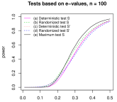
Replacing by , we obtain the new e-process by The e-process is not growth optimal, but as satisfies (DE), we can test via the rejection condition , thus boosting the terminal value by a factor of . Let be independent of the test statistics. We compare five different tests, all with size at most :
-
(a)
applying (12) to : reject if (benchmark case);
-
(b)
applying (13) to : reject if ;
-
(c)
applying (14) to : reject if ;
- (d)
-
(e)
applying (15) to the maximum of : reject if .
Since test (a) is strictly dominated by test (e), we do not need to use (a) in practice; nevertheless we treat it as a benchmark for comparison on tests based on e-values as it is built on the fundamental connection between e-values and p-values: the e-to-p calibrator .
The significance level is set to be . The power of the five tests is computed from the average of 10,000 replications for varying signal strength and for . Results are reported in Figure 3. For most values of and , either the deterministic test (c) for or the maximum test (e) has the best performance. The deterministic test (c) performs very well in the cases and , especially for weak signals; this may be explained by the factor of being substantial when the signal is weak. If is large and the signal is not too weak, the effect of using the maximum of in (e) is dominating; this is not surprising. Although the randomized test (b) usually improves the performance from the benchmark case (a), the advantages seem to be quite limited, especially in view of the extra randomization, often undesirable.


8 Testing with combined mid p-values
We compare by simulation the performance of a few tests via merging mid p-values. The (global) null hypothesis is that the test statistic follows a binomial distribution , and tests are conducted. We set and , so that the obtained p-values are considerably discrete. We denote by the obtained p-values via (2), and the obtained mid p-values via (3). Let and be the arithmetic average and the geometric average of , respectively.
The true data probability generating the test statistics is a binomial distribution , where . The case means that the null hypothesis is true, and a larger indicates a stronger signal.
We allow the test statistics to be correlated, and this is achieved by simulating from a Gaussian copula with common pairwise correlation parameter (more precisely, we first simulate from a Gaussian copula, and then obtain the observable discrete test statistics by a quantile transform). We consider the following tests (there are other tests possible for this setting, and we only compare these four to illustrate a few relevant points):
- (a)
-
(b)
the arithmetic mean times using Proposition 5.3: reject if ;
-
(c)
the geometric average of p*-values using Theorem 5.2: reject if ;
-
(d)
the Bonferroni correction: reject if .
Note that tests (a), (b) and (c) use mid p-values based on methods for p*-values, and (d) uses p-values. All of (b), (c) and (d) are valid tests under arbitrary dependence (AD) whereas the validity of (a) requires independence. Therefore, we expect (a) to perform very well in case independence holds. All other methods are valid but conservative, as there is a big price to pay to gain robustness against all dependence structures.
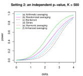
The significance level is set to be for good visibility. The power of the four tests is reported in Figure 4 which is computed from the average of 10,000 replications for varying signal strength and for (independence), (mild dependence) and (strong dependence). The situation of is the most relevant to us as averaging methods are designed mostly for situations where the presence of strong or complicated dependence is suspected.


As we can see from Figure 4, the test (a) relying on independence has the strongest power as expected. Its size becomes largely inflated as soon as mild dependence is present, and hence it can only be applied in situations where independence among obtained mid p-values can be justified. Indeed, the size of test (a) can be in case , which is clearly not useful. Among the three methods that are valid for arbitrary dependence, the geometric average (c) has stronger power for large and the Bonferroni correction (d) has stronger power for small . The arithmetic average (b) performs poorly unless p-values are very strongly correlated. These observations on merging mid p-values are consistent with those in [34] on merging p-values. In conclusion, the geometric average (c) can be useful when the dependence among mid p-values is speculated to be strong or complicated, although unknown to the decision maker.
9 Conclusion
In this paper we introduced p*-values (p*-variables) as an abstract measure-theoretic object. The notion of p*-values is a manifold generalization of p-values, and it enjoys many attractive theoretical properties in contrast to p-values. In particular, mid p-values, which arise in the presence of discrete test statistics, form an important subset of p*-values. Merging methods for p*-values are studied. In particular, a weighted geometric average of arbitrarily dependent p*-values multiplied by yields a valid p-value, which can be useful when multiple mid p-values are possibly strongly correlated.
Results on calibration between p*-values and e-values reveal that p*-values serve as an intermediate step in both the standard e-to-p and p-to-e calibrations. Although a direct test with p*-values may involve randomization, we find that p*-values are useful in the design of deterministic tests with averages of p-values, mid p-values, and e-values. From the results in this paper, the concept of p*-values serves a useful technical tool which enhances the extensive and growing applications of p-values, mid p-values, and e-values.
[Acknowledgments] The author thanks Ilmun Kim, Aaditya Ramdas, and Vladimir Vovk for constructive comments on an earlier version of the paper, and Tiantian Mao, Marcel Nutz, and Qinyu Wu for kind help on some technical statements.
The author acknowledges financial support from and the Natural Sciences and Engineering Research Council of Canada (RGPIN-2018-03823, RGPAS-2018-522590).
References
- [1]
- Bates et al. [2021] Bates, S., Candès, E., Lei, L., Romano, Y. and Sesia, M. (2021). Testing for outliers with conformal p-values. arXiv: 2104.08279.
- Benjamini and Hochberg [1995] Benjamini, Y. and Hochberg, Y. (1995). Controlling the false discovery rate: A practical and powerful approach to multiple testing. Journal of the Royal Statistical Society Series B, 57(1), 289–300.
- Benjamini and Hochberg [1997] Benjamini, Y. and Hochberg, Y. (1997). Multiple hypotheses testing with weights. Scandinavian Journal of Statistics, 24(3), 407–418.
- Benjamini and Yekutieli [2001] Benjamini, Y. and Yekutieli, D. (2001). The control of the false discovery rate in multiple testing under dependency. Annals of Statistics, 29(4), 1165–1188.
- Chen et al. [2022] Chen, Y., Liu, P. and Tan, K. S. and Wang, R. (2022). Trade-off between validity and efficiency of merging p-values under arbitrary dependence. Statistica Sinica, forthcoming.
- Howard et al. [2021] Howard, S. R., Ramdas, A., McAuliffe, J. and Sekhon, J. (2021). Time-uniform, nonparametric, nonasymptotic confidence sequences. Annals of Statistics, 49(2), 1055–1080.
- Döhler et al. [2018] Döhler, S., Durand, G. and Roquain, E. (2018). New FDR bounds for discrete and heterogeneous tests. Electronic Journal of Statistics, 12(1), 1867–1900.
- Duan et al. [2020] Duan, B., Ramdas, A., Balakrishnan, S. and Wasserman, L. (2020). Interactive martingale tests for the global null. Electronic Journal of Statistics, 14(2), 4489–4551.
- Efron [2010] Efron, B. (2010). Large-scale Inference: Empirical Bayes Methods for Estimation, Testing, and Prediction. Cambridge University Press.
- Genovese and Wasserman [2004] Genovese, R. and Wasserman, L. (2004). A stochastic process approach to false discovery control. Annals of Statistics, 32, 1035–1061.
- Goeman and Solari [2011] Goeman, J. J. and Solari, A. (2011). Multiple testing for exploratory research. Statistical Science, 26(4), 584–597.
- Grünwald et al. [2020] Grünwald, P., de Heide, R. and Koolen, W. M. (2020). Safe testing. arXiv: 1906.07801v2.
- Habiger [2015] Habiger, J. D. (2015). Multiple test functions and adjusted p-values for test statistics with discrete distributions. Journal of Statistical Planning and Inference, 167, 1–13.
- Huber [2019] Huber, M. (2019). Halving the bounds for the Markov, Chebyshev, and Chernoff Inequalities using smoothing. The American Mathematical Monthly, 126(10), 915–927.
- Lancaster [1952] Lancaster, H. O. (1952). Statistical control of counting experiments. Biometrika, 39(3/4), 419–422.
- Liu and Wang [2021] Liu, F. and Wang, R. (2021). A theory for measures of tail risk. Mathematics of Operations Research, 46(3), 1109–1128.
- Liu and Xie [2020] Liu, Y. and Xie, J. (2020), Cauchy combination test: A powerful test with analytic p-value calculation under arbitrary dependency structures. Journal of the American Statistical Association, 115(529), 393–402.
- Mao et al. [2019] Mao, T., Wang, B. and Wang, R. (2019). Sums of uniform random variables. Journal of Applied Probability, 56(3), 918–936.
- Meng [1994] Meng, X. L. (1994). Posterior predictive -values. Annals of Statistics, 22(3), 1142–1160.
- Müller and Stoyan [2002] Müller, A. and Stoyan, D. (2002). Comparison Methods for Stochastic Models and Risks. Wiley, England.
- Ramdas et al. [2019] Ramdas, A. K., Barber, R. F., Wainwright, M. J. and Jordan, M. I. (2019). A unified treatment of multiple testing with prior knowledge using the p-filter. Annals of Statistics, 47(5), 2790–2821.
- Rubin-Delanchy et al. [2019] Rubin-Delanchy, P., Heard, N. A. and Lawson, D. J. (2019). Meta-analysis of mid-p-values: Some new results based on the convex order. Journal of the American Statistical Association, 114(527), 1105–1112.
- Rüschendorf [1982] Rüschendorf, L. (1982). Random variables with maximum sums. Advances in Applied Probability, 14(3), 623–632.
- Rüschendorf [2013] Rüschendorf, L. (2013). Mathematical Risk Analysis. Dependence, Risk Bounds, Optimal Allocations and Portfolios. Springer, Heidelberg.
- Sarkar [1998] Sarkar, S. K. (1998). Some probability inequalities for ordered MTP2 random variables: a proof of the Simes conjecture. Annals of Statistics, 26(2), 494–504.
- Shafer [2021] Shafer, G. (2021). The language of betting as a strategy for statistical and scientific communication. Journal of the Royal Statistical Society Series A, 184(2), 407–431.
- Shafer et al. [2011] Shafer, G., Shen, A., Vereshchagin, N. and Vovk, V. (2011). Test martingales, Bayes factors, and p-values. Statistical Science, 26, 84–101.
- Shaked and Shanthikumar [2007] Shaked, M. and Shanthikumar, J. G. (2007). Stochastic Orders. Springer Series in Statistics.
- Simes [1986] Simes, R. J. (1986). An improved Bonferroni procedure for multiple tests of significance. Biometrika, 73, 751–754.
- Vovk [2020] Vovk, V. (2020). Testing randomness online. Statistical Science, 36(4), 595–611.
- Vovk et al. [2005] Vovk, V., Gammerman, A. and Shafer, G. (2005). Algorithmic Learning in a Random World. Springer, New York.
- Vovk et al. [2022] Vovk, V., Wang, B. and Wang, R. (2022). Admissible ways of merging p-values under arbitrary dependence. Annals of Statistics, 50(1), 351–375.
- Vovk and Wang [2020] Vovk, V. and Wang, R. (2020). Combining p-values via averaging. Biometrika, 107(4), 791–808.
- Vovk and Wang [2021] Vovk, V. and Wang, R. (2021). E-values: Calibration, combination, and applications. Annals of Statistics, 49(3), 1736–1754.
- Wang and Wang [2015] Wang, B. and Wang, R. (2015). Extreme negative dependence and risk aggregation. Journal of Multivariate Analysis. 136, 12–25.
- Wang and Ramdas [2022] Wang, R. and Ramdas, A. (2022). False discovery rate control with e-values. Journal of the Royal Statistical Society Series B, forthcoming.
- Wasserman et al. [2020] Wasserman, L., Ramdas, A. and Balakrishnan, S. (2020). Universal inference. Proceedings of the National Academy of Sciences, 117(29), 16880–16890.
- Wilson [2019] Wilson, D. J. (2019). The harmonic mean p-value for combining dependent tests. Proceedings of the National Academy of Sciences, 116, 1195–1200.
Appendix A Proofs of all results
In this appendix, we collect proofs of all theorems and propositions in the main paper.
A.1 Proofs of results in Section 3
Proof of Theorem 3.1.
-
(i)
For being a strictly increasing function of , we have , and the equivalence statement follows directly from the definition of p-variables.
-
(ii)
We first show the “if” statement. Write for an increasing function . Denote by and the distribution function and the left-quantile function of , respectively, and let be a standard uniform random variable independent of . Moreover, let
which is uniformly distributed on and satisfies a.s. (e.g., [25, Proposition 1.3]). Since a.s., and both and are increasing, we know that the functions and differ on a set of Lebesgue measure . Therefore, , which is identically distributed as . Moreover,
(17) Therefore, implies , and thus is a mid p-variable.
The “only if” statement follows from and (17) by choosing and .
-
(iii)
We first show the “if” statement. Note that where the second inequality is guaranteed by Jensen’s inequality. Since is stronger than and is transitive, we get and hence is a p*-variable.
Next, we show the “only if” statement. By using [29, Theorems 4.A.5], the definition of a p*-variable implies that there exist a standard uniform random variable and a random variable such that . ∎
Proof of Proposition 3.3.
By Theorem 4.1, the set of p*-variables is the convex hull of the set of p-variables, and thus convex. This also implies that none of the set of p-variables or that of mid p-variables is convex.
To show that the set of p*-variables is closed under distribution mixtures, it suffices to note that the stochastic orders and (indeed, any order induced by inequalities via integrals) is closed under distribution mixture.
To see that the set of mid p-variables is not closed under distribution mixtures, we note from (3) that any mid p-variable with mean and a point-mass at must not have any density in a neighbourhood of . Hence, the mixture of uniform distribution on and a point-mass at is not the distribution of a mid p-variable.
Closure under convergence for is justified by Theorem 1.A.3 of [29], and closure under convergence for is justified by Theorem 1.5.9 of [21]. Closure under convergence for the set of mid p-values follows by noting that the set of distributions of in (3) is closed under convergence in distribution, which can be checked by definition. ∎
A.2 Proofs of results in Section 4
Proof of Theorem 4.1.
We first show that a convex combination of p-variables is a p*-variable. Let be a uniform random variable on , be p-variables, be an element of the standard -simplex, and be an increasing concave function. By monotonicity and concavity of , we have
Therefore, and thus is a p*-variable.
Next, we show the second statement that any p*-variable can be written as the average of three p-variables, which also justifies the “only if” direction of the first statement.
Let be a p*-variable satisfying . Note that and together implies (see e.g., [29, Theorem 4.A.35]), where is the concave order, meaning that for all concave . Theorem 5 of [19] says that any , there exist three standard uniform random variables such that (this statement is highly non-trivial). This implies that can be written as the arithmetic average of three p-variables .
Finally, assume that the p*-variable satisfies . In this case, using Strassen’s Theorem in the form of [29, Theorems 4.A.5 and 4.A.6], there exists a random variable such that . As we explained above, there exist p-variables such that . For , let . Note that are p-variables and . Hence, can be written as the arithmetic average of three p-variables. ∎
Proof of Proposition 4.3.
For the “only-if” statement in (i), since is a p-variable, we know that its distribution satisfies for . Therefore, by setting ,
where the last equality holds since is independent of . To check the “if” direction of (i), we have where is the distribution of . Note that is stochastically larger than or equal to a uniform random variable on , and hence .
Next, we show (ii). First, suppose that . Let be a uniform random variable on . By Jensen’s inequality, we have . Hence, , and thus is a p*-variable.
For the converse direction, suppose that is a p*-variable. By Strassen’s Theorem in the form of [29, Theorem 3.A.4], there exists a uniform random variable on and a random variable identically distributed as such that . Let be the left-quantile function of a regular conditional distribution of given . Further, let be a uniform random variable on independent of , and . It is clear that has the same law as . Therefore, . Moreover, since is independent of . Hence, . Let be another uniform random variable on independent of . We have
Hence, the representation holds with and .
Finally, we show the last statement on replacing by . The “only-if” direction follows from the argument for (ii) by noting that constructed above has a continuous distribution. The “if” direction follows from
where the second-last inequality is Jensen’s, and the last inequality is implied by Theorem 3.1. ∎
Proof of Proposition 4.5.
The “if” statement is implied by Proposition B.1. To show the “only if” statement, denote by the distribution function of and be the distribution function of a uniform random variable on . We have
Therefore, for , we have
By Theorem 4.A.2 of [29], the above inequality implies . Hence, is a p*-variable. ∎
A.3 Proofs of results in Section 5
Proof of Proposition 5.1.
Let be a uniform random variable on . The first statement is trivial by definition. For the second statement, let be two p*-variables. For any ,
where the last inequality is because and is convex and decreasing. Therefore, is a p-variable. ∎
The following lemma is needed in the proof of Theorem 5.2.
Lemma A.1.
Let be an increasing Borel function on . Then is a p-variable for all p*-variables if and only if
| (18) |
where is uniform on and is the essential supremum of a random variable .
Proof.
Let be the critical value for testing with , that is, the largest value such that
Converting between the distribution function and the quantile function, this means
where be the left -quantile of a random variable . For an increasing function , its infimum -quantile can be converted to the essential supremum of random variables with conditional distributions on their lower -tail; see the proof of [17, Theorem 3] which deals with the case of additive functions (see also the proof of [6, Proposition 1] where this technique is used). Note that for , its lower -tail conditional distribution dominates . This argument leads to
Noting that is equivalent to , we obtain (18). ∎
Proof of Theorem 5.2.
First, suppose that are non-negative constants adding up to . Let be the critical value for testing with , that is, the smallest value such that
We will show that . Using Lemma A.1, we get
For any p*-variables , since is an increasing concave function, we have
Therefore, , leading to the desired bound , and thus
For random , taking an expectation leads to (6). ∎
Proof of Proposition 5.3.
The validity of as a p*-merging function is implied by Theorem 4.1. To show its admissibility, suppose that there exists a p*-merging function that strictly dominates . Let be iid uniform random variables on . The strict domination implies and . We have
This means that is not a p*-variable, a contradiction. ∎
Proof of Proposition 5.4.
Let be p*-variables, and be a random variable such that the distribution of is the equally weighted mixture of those of . Note that a p*-variable by Proposition 3.3. Let . Using the Bonferroni inequality, we have, for any ,
| (19) |
Let be the left-quantile function of and be that of . By (19), we have for all . Hence, for each , using the equivalent condition (1), we have
This implies, via the equivalent condition (1) again, that is a p*-variable.
Next we show the admissibility of for , since the case is trivial. Suppose that there is a p*-merging function which strictly dominates . Since is increasing, there exists such that . First, assume . Define identically distributed random variables by
where are disjoint events with for each . It is easy to check that are p*-variables, and
Thus, takes the value with probability , and it takes the value otherwise. Let be the left-quantile function of . The above calculation leads to
showing that is not a p*-variable by (1), a contradiction.
Next, assume . In this case, let , and define identically distributed random variables by
where are disjoint events with and , . Note that the union of has probability . It is easy to verify that are p*-variables. Moreover, we have since dominates . Hence, takes the value with probability , and it takes the value otherwise. Let be the left-quantile function of . Using and , we obtain
showing that is not a p*-variable by (1), a contradiction. As cannot strictly dominate , we know that is admissible. ∎
A.4 Proofs of results in Section 6
Proof of Theorem 6.1.
Let be a uniform random variable on .
-
(i)
The validity of the calibrator is implied by (i), and below we show that it dominates all others. For any function on , suppose that for some . Consider the random variable defined by . Clearly, is a p*-variable. Note that
implying that is not a p*-to-p calibrator. Hence, any p*-to-p calibrator satisfies for all , thus showing that dominates all p*-to-p calibrators.
-
(ii)
By (1), we know that , and thus is a valid p-to-p* calibrator. To show its admissibility, it suffices to notice that is left-continuous (lower semi-continuous) function on , and if and , then , implying that cannot be a p*-variable. ∎
Proof of Theorem 6.2.
-
(i)
Let be a convex p-to-e calibrator. Note that is increasing and concave. For any -valued p*-variable , by definition, we have Hence,
Since a -valued p*-variable is first-order stochastically larger than some -valued p*-variable (e.g., [29, Theorem 4.A.6]), we know that for all p*-variables . Thus, is a p*-to-e calibrator.
Next, we show the statement on admissibility. A convex admissible p-to-e calibrator is a p*-to-e calibrator. Since the class of p-to-e calibrators is larger than the class of p*-to-e calibrators, is not strictly dominated by any p*-to-e calibrator.
-
(ii)
We only need to show the “only if” direction, since the “if” direction is implied by (i). Suppose that a non-convex function is an admissible p-to-e calibrator. Since is not convex, there exist two points such that
Left-continuity of implies that there exists such that
Note that
and the inequality also holds if the positions of and are flipped. Hence, by letting , we have
(20) Let be a uniform random variable on and be given by
For any increasing concave function and and , we have
Therefore, , and hence . Thus, is a p*-variable. Moreover, using (20), we have
Hence, is not a p*-to-e calibrator. Thus, has to be convex if it is both an admissible p-to-e calibrator and a p*-to-e calibrator.
-
(iii)
First, we show that is an e-to-p* calibrator. Clearly, it suffices to show that is a p*-variable for any e-variable with mean , since any e-variable with mean less than is dominated by an e-variable with mean . Let be the point-mass at .
Assume that has a two-point distribution (including the point-mass as a special case). With , the distribution of can be characterized with two parameters and via
The distribution of (we allow to take the value in case ) is given by
Let be the left-quantile function of on . We have
Define two functions and on by and . For , we have, using ,
Moreover, Jensen’s inequality gives
Since is linear on , and is convex, and imply for all . Therefore, we conclude that on , namely
Using (1), we have that is a p*-variable.
For a general e-variable with mean , its distribution can be rewritten as a mixture of two-point distributions with mean (see e.g., the construction in Lemma 2.1 of [36]). Since the set of p*-variables is closed under distribution mixtures (Proposition 3.3), we know that is a p*-variable. Hence, is an e-to-p* calibrator.
To show that essentially dominates all other e-to-p* calibrators, we take any e-to-p* calibrator . Using Theorem 6.1, the function is an e-to-p calibrator. Using Proposition 2.2 of [35], any e-to-p calibrator is dominated by , and hence
which in term gives for . Since is decreasing, we know that implies . For any with , we have , and thus essentially dominates . ∎
Proof of Proposition 6.4.
Appendix B Randomized p*-test and applications
In this appendix we discuss several applications of testing with p*-values and randomization.
B.1 Randomized p*-test
We first introduce the a generalized version of the randomized p*-test in Proposition 4.5. The following density condition (DP) for a -valued random variable will be useful.
-
(DP)
has a decreasing density function on .
The canonical choice of satisfying (DP) is a uniform random variable on for , which we will explain later. For a -valued random variable with mean and a p*-variable independent of , we consider the test
| (21) |
The following theorem justifies the validity of the test (21) with the necessary and sufficient condition (DP).
Proposition B.1.
The proof of Proposition B.1 relies on the following lemma.
Lemma B.2.
For any non-negative random variable with a decreasing density function on (with possibly a probability mass at ) and any p*-variable independent of , we have .
Proof.
Let be the distribution function of , which is an increasing concave function on because of the decreasing density. Since is a p*-variable, we have . Therefore,
Hence, the statement in the lemma holds. ∎
Proof of Proposition B.1.
We first note that (ii) is straightforward: for a uniform random variable on independent of , then . If , then .
The “if” statement of point (i) directly follows from Lemma B.2, noting that condition (DP) is stronger than the condition in Lemma B.2. Below, we show the “only if” statement of point (i).
Let be the distribution function of and be a uniform random variable on . Suppose that is not concave on . It follows that there exists such that . By the right-continuity of , there exists such that
| (22) |
Let and , which are disjoint intervals. Define a random variable by
| (23) |
We check that defined by (23) is a p*-variable. For any concave function , Jensen’s inequality gives
Hence, is a p*-variable. It follows from (22) and (23) that
Therefore,
Since this contracts the validity requirement, we know that has to have a concave distribution function, and hence a decreasing density on . ∎
Lemma B.2 gives for possibly taking values larger than and possibly having a probability mass at . We are not interested designing a random threshold with positive probability to be or larger than , but this result will become helpful in Section 7. Since condition (DP) implies , we will assume , which is certainly harmless for practice.
With the help of Proposition B.1, we formally define -random thresholds and the randomized p*-test.
Definition B.3.
For a significance level , an -random threshold is a -valued random variable independent of the test statistics (a p*-variable in this section) with mean satisfying (DP). For an -random threshold and a p*-variable , the randomized p*-test is given by (21), i.e., rejecting the null hypothesis .
Proposition B.1 implies that the randomized p*-test always has size at most , just like the classic p-test (4). Since the randomized p*-test (21) has size equal to if is uniformly distributed on , the size of the randomized p*-test cannot be improved in general.
As mentioned in Section 4.4, randomization is generally undesirable in testing. Like any other randomized methods, different scientists may arrive at different statistical conclusions by the randomized p*-test for the same data set generating the p*-value. Because of assumption (DP), which is necessary for validity by Proposition B.1, we cannot reduce the -random threshold to a deterministic . This undesirable feature is the price one has to pay when a p-variable is weakened to a p*-variable.
If one needs to test with a deterministic threshold, then needs to be used instead of . In other words, the test
| (24) |
has size for all p*-variable . The validity of (24) was noted by Rüschendorf [24], and it is a direct consequence of Proposition 5.1. Unlike the random threshold which gives a size precisely in realistic situations, the deterministic threshold is often overly conservative in practice (see discussions in [20, Section 5]), but it cannot be improved in general when testing with the average of p-variables ([34, Proposition 3]); recall that the average of p-variables is a p*-variable.
We will see an application of the randomized p*-test in Section B.2, leading to new tests on the weighted average of p-values, which can be made deterministic if one of the p-values is independent of the others. Moreover, the randomized p*-test can be used to improve the power of tests with e-values and martingales in Section 7.
As mentioned above, the extra randomness introduced by the random threshold is often considered undesirable. One may wish to choose such that the randomness is minimized. The next result shows that is the optimal choice if the randomness is measured by variance or convex order.
Proposition B.4.
For any -random threshold , we have , and this smallest variance is attained by . Moreover, for any convex function (hence holds).
Proof.
We directly show for all convex functions , which implies the statement on variance as a special case since the mean of is fixed as . Note that has a concave distribution function on , and has a linear distribution function on . Moreover, they have the same mean. Hence, there exists such that for and for . This condition is sufficient for by Theorem 3.A.44 of [29]. ∎
Combining Propositions B.1 and B.4, the canonical choice of the threshold in the randomized p*-test has a uniform distribution on .
We note that it is also possible to use some with mean less than and variance less than . This reflects a tradeoff between power and variance. Such a random threshold does not necessarily have a decreasing density. For instance, the point-mass at is a valid choice; the next proposition gives some other choices.
Proposition B.5.
Let be an -random threshold and is a random variable satisfying . We have for arbitrary p*-variable independent of .
Proof.
Let be the distribution function of . For any increasing function , we have , which follows from . Hence, we have
where the last inequality follows from Proposition B.1. ∎
Proposition B.5 can be applied to a special situation where a p-variable and an independent p*-variable are available for the same null hypothesis. Note that in this case . Hence, by Proposition B.5, the test
| (25) |
has size at most . Alternatively, using the fact that implied by Proposition B.1 (ii), we can design a test
| (26) |
The tests (25) and (26) both have a deterministic threshold of . This observation is useful in Section B.2.
B.2 Testing with averages of p-values
In this section we illustrate applications of the randomized p*-test to tests with averages of dependent p-values.
Let be p-variables for a global null hypothesis and they are generally not independent. Vovk and Wang [34] proposed testing using generalized means of the p-values, so that the type-I error is controlled at a level under arbitrary dependence. We focus on the weighted (arithmetic) average for some weights with . In case , we speak of the arithmetic average.
The method of [34] on arithmetic average is given by
| (27) |
We will call (27) the arithmetic averaging test. The extra factor of is needed to compensate for arbitrary dependence among p-values. Since is a p*-variable by Theorem 4.1, the test (27) is a special case of (24). This method is quite conservative, and it often has relatively low power compared to the Bonferroni correction and other similar methods unless p-values are very highly correlated, as illustrated by the numerical experiments in [34].
To enhance the power of the test (27), we apply the randomized p*-test in Section 4.4 to design the randomized averaging test by
| (28) |
where is an -random threshold independent of . Comparing the fixed-threshold test (27) and the randomized averaging test (28) with , there is a probability that the randomized averaging test has a better power, with the price of randomization.
Next, we consider a special situation, where a p-variable among is independent of the others under the null hypothesis. In this case, we can apply (25), and the resulting test is no longer randomized, as it is determined by the observed p-values.
Without loss of generality, assume that is independent of . Let be a weighted average of . Using as the p*-variable, the test (25) becomes
| (29) |
Following directly from the validity of (25), for any p-variables with independent of , the test (29) has size at most .
B.3 Simulation experiments
We compare by simulation the performance of a few tests via merging p-values. For the purpose of illustration, we conduct correlated z-tests for the mean of normal samples with variance . More pecisely, the null hypothesis is and the alternative is for some . The p-variables are specified as from the Neyman-Pearson lemma, where is the standard normal distribution function, and are generated from with pair-wise correlation . As illustrated by the numerical studies in [34], the arithmetic average test performs poorly unless p-values are strongly correlated. Therefore, we consider the cases where p-values are highly correlated, e.g., parallel experiments with shared data or scientific objects. We set in our simulation studies; this choice is harmless as we are interested in the relative performance of the averaging methods in this section, instead of their performance against other methods (such as method of Simes [30]) that are known work well for lightly correlated or independent p-values.
The significance level is set to be . For a comparison, we consider the following tests:
-
(a)
the arithmetic averaging test (27): reject if ;
-
(b)
the randomized averaging test (28): reject if where independent of ;
-
(c)
the Bonferroni method: reject if ;
-
(d)
the Simes method: reject if where is the -th smallest p-value;
- (e)
The validity (size no larger than ) of the Simes method is guaranteed under some dependence conditions on the p-values; see [26, 5]. Moreover, as shown recently by Vovk et al. [33, Theorem 6], the Simes method dominates any symmetric and deterministic p-merging method valid for arbitrary dependence (such as the (a), (c) and (e); the Simes method itself is not valid for arbitrary dependence).
In the second setting, we assume that one of the p-variables ( without loss of generality) is independent of the rest, and the rest p-variables have a pair-wise correlation of . For this setting, we further include
-
(f)
the enhanced averaging test (29): reject if .
The power (i.e., the probability of rejection) of each test is computed from the average of 10,000 replications for varying signal strength and for . Results are reported in Figure 5.
In the first setting of correlated p-values, the randomized averaging test (b) improves the performance of (a) uniformly, at the price of randomization. The Bonferroni method (d) and the harmonic averaging test (e) perform poorly and are both penalized significantly as increases. None of these methods visibly outperforms the Simes method, although in some situations the test (b) performs comparably to the Simes method.
In the second setting where an independent p-value exists, the enhanced arithmetic test (f) performs quite well; it outperforms the Simes method for most parameter values especially for small signal strength . This illustrates the significant improvement via incorporating an independent p-value.
We remark that the averaging methods (a), (b) and (f) should not be used in situations in which correlation among p-values is known to be not very strong. This is because the arithmetic mean does not benefit from an increasing number of independent p-values of similar strength, unlike the methods of Bonferroni and Simes.