Testing the microstructure of $d$-dimensional charged Gauss-Bonnet anti-de Sitter black holes

The line element for the black hole is Boulware ; Cai2 ; Wiltshire ; Cvetic2

where $M$ and $Q$ are the mass and charge of the black hole, respectively. The parameter $\alpha$ is related with the GB coupling $\alpha=(d-3)(d-4)\alpha_{\text{GB}}$ with dimension [length]². The volume of the unit $(d-2)$-sphere is $\omega_{d-2}=2\pi^{(d-1)/2}/\Gamma((d-1)/2)$. Here we consider the thermodynamic quantity in the extended phase space, where the cosmological constant $\Lambda$ has been interpreted as the pressure $P=-\frac{\Lambda}{8\pi}$. This solution is obtained from the following action

where the GB Lagrangian $\mathcal{L}_{\text{GB}}=\mathcal{R}_{\mu\nu\gamma\delta}\mathcal{R}^{\mu\nu\gamma\delta}-4\mathcal{R}_{\mu\nu}\mathcal{R}^{\mu\nu}+\mathcal{R}^{2}$.

The radius of the event horizon can be obtained by solving $f(r_{\text{h}})=0$, which depends on the black hole mass, charge and pressure. Here we can also express the black hole mass as

Other thermodynamic quantities, such as the temperature $T$, entropy $S$, electric potential $\Phi$, and conjugate quantity $\mathcal{A}$ to $\alpha$ are given by Cai

The specific volume and thermodynamic volume are given by

It is clear that $V\sim v^{d-1}$, so they are not linear, which is quite different from the VdW fluid. For the black hole thermodynamics, these two volumes have different applications, see the related discussion in Ref. Wei3 . One can easily confirm that the first law and the Smarr formula hold

From (11), we find that the pressure-volume term is $VdP$ rather than $-PdV$. So, as suggested in Ref. Kastor , the black hole mass $M$ here should be treated as the enthalpy $H$ of the system.

Solving Eq. (5), we can obtain the equation of state

Obviously, this equation closely depends on the GB coupling $\alpha$ and charge $Q$. According to the classification of the black hole quantities Wei6 , this black hole system is a double characteristic parameter system. However, we can reduce these thermodynamic quantities with the charge $Q$. This shall help us to simplify the study. Via the dimensional analysis, we adopt the following reduced forms

Then the reduced equation of state reads

Now we find that the equation of state only depends on the reduced GB coupling $\tilde{\alpha}=\alpha/Q^{2/(d-3)}$. Moreover, we can express the reduced pressure in terms of the thermodynamic volume $\tilde{V}$. Another important thermodynamic quantity is the Gibbs free energy, which is

The local thermodynamic stability is measured by the heat capacity. Positive or negative one indicates the system is local stable or unstable. The heat capacity can be calculated by

Since it is in a complex form, we shall not show it here. In the following section, we will investigate the phase structure for different dimension number $d$.

In this subsection, we would like to give a brief introduction for the Ruppeiner geometry, and to show how black hole microstructure is uncovered via the geometry.

Here we consider that the system S we concerned is surrounded by its huge environment E. Then the total entropy of the complete system can be written as

where we assume the system has two independent thermodynamic extensive variables $x^{0}$ and $x^{1}$. Moreover, $S_{\rm S}\ll S_{\rm E}\sim S$ is required. Near the local maximum of the entropy at $x^{\mu}=x^{\mu}_{0}$, we expand the total entropy as

where we denote the local maximum of the entropy $S(x^{\mu}_{0})$ with $S_{0}$. Since the fluctuating parameters are additive, i.e., $x_{S}^{\mu}+x_{E}^{\mu}=x_{total}^{\mu}=constant$, one can easily get $\left.\frac{\partial S_{\rm S}}{\partial x^{\mu}}\right|_{0}\Delta x^{\mu}_{\rm S}+\left.\frac{\partial S_{\rm E}}{\partial x^{\mu}}\right|_{0}\Delta x^{\mu}_{\rm E}=0$. Thus we have $\Delta S=S-S_{0}$,

The second term is much smaller than the first term, so we ignore it. Finally, the probability of finding the system in the internals $x_{0}\sim(x_{0}+\Delta x_{0})$ and $x_{1}\sim(x_{1}+\Delta x_{1})$ can be expressed in the following form

where

According to the thermodynamic information geometry, $\Delta l^{2}$ measures the distance between two neighboring fluctuation states. The less probable a fluctuation between two neighboring states, the longer the distance between them. Following the Riemannian geometry, we can construct the corresponding scalar curvature for this Ruppeiner geometry. The empirical observation suggests that positive (negative) scalar curvature indicates the repulsive (attractive) interaction among the small molecules of the system. Further study also uncovers that the scalar curvature is related to the correlation length for the thermodynamic system near the critical point.

Taking the internal energy $U$ and thermodynamic volume $V$ as the fluctuation coordinates, the line element can be reexpressed via the first law of the black hole thermodynamics as

where the free energy $F=U-TS$ and it satisfies the differential law $dF=-SdT-PdV$. By making use of the heat capacity at constant volume $C_{V}=T(\partial_{T}S)_{V}$, the line element reads

The scalar curvature for this geometry is WeiWeiWei

Similar to the charged AdS black holes, here we also have $C_{V}$=0 for the charged GB-AdS black holes. This will lead to the divergence of $R$. In order to uncover the specific properties hiding behind it, we have defined a new normalized scalar curvature, which is

Adopting this normalized scalar curvature, the microstructure has been explored for several different black holes.

For $d$=5, the reduced equation of state, the Gibbs free energy, and the heat capacity are given by

The equation of state (28) exhibits a small-large black hole phase transition, reminiscent of the liquid-gas phase transition of the VdW fluid. For the phase transition, there is a characteristic critical point indicating a second-order phase transition, which can be determined by

Since $V=\frac{\pi^{2}}{2}r_{\text{h}}^{4}$ for $d$=5, the conditions can be expressed as

Solving the equation, we have

Then the critical value of the radius of the horizon can be obtained

The corresponding critical pressure and temperature are

We plot the critical point in the $\tilde{P}$-$\tilde{T}$ diagram in Fig. 1 for varying $\tilde{\alpha}$. When $\tilde{\alpha}$=0, the critical point curve starts at ($\frac{4}{5\sqrt[4]{5}\pi}$, $\frac{1}{4\sqrt{5}\pi}$). Then with the increase of $\tilde{\alpha}$, the curve extends to low temperature and pressure, and ends at (0, 0) when $\tilde{\alpha}\rightarrow\infty$. Each point on this curve is a phase transition point of second-order.

For $\tilde{\alpha}$=0.4 and 1.4, we plot the heat capacity in Fig. 2 when the pressure takes its critical values. Obviously, we observe the $\lambda$ behaviors for these two cases. Such pattern of the heat capacity is reminiscent of that of ⁴He. For black hole systems, this behavior was first observed in Ref. Tjoa2 , where a new superfluid was uncovered. Here, we suggest that such $\lambda$ behavior of the heat capacity implies a second-order phase transition rather a new black hole phase unless the conditions given in Ref. Tjoa2 are satisfied.

Employing these critical thermodynamic quantities, we can construct a universal quantity

For $\alpha$=0, we have $\rho$=5/16.

Next, we plot the isothermal curves and the Gibbs free energies for further understanding the black hole phase transition. The isothermal curves are shown in Fig. 3 in the $\tilde{P}$-$\tilde{V}$ diagram for $\tilde{\alpha}$=0.4 and 1.4, respectively. From these figures, one can observe nonmonotonic behavior for low temperature, which indicates the existence of the small-large phase transition. For fixed temperature, these black hole branches of the positive slope are nonphysical. They should be removed by other mechanisms, one of which is the Maxwell equal area law. One can draw a horizontal line to construct two equal areas on one isothermal curve. Then the pressure and temperature corresponding to the horizontal line denote the values of the phase transition point. In our reduced treatment, it is equivalent to fix the charge, so the equal area law is also applicable in the $\tilde{P}$-$\tilde{V}$ diagram on determining the phase transition point.

Another alternative on determining the phase transition is the Gibbs free energy. We show its behavior in Fig. 4. When the temperature is lower than the critical value, there is the characteristic swallow tail behavior. Combining the thermodynamic choice that a system always prefers the lowest free energy, the phase transition exactly occurs at the intersection point of the Gibbs free energy. Therefore, one can also use such property to numerically solve the phase transition point.

Actually, these two approaches coincide with each other when the first law of the black hole thermodynamics holds. Here we display the phase structures in the $\tilde{P}$-$\tilde{T}$ and $\tilde{T}$-$\tilde{r}_{\text{h}}$ diagrams in Figs. 5 and 6, respectively. In the $\tilde{P}$-$\tilde{T}$ diagram shown in Fig. 5, the red solid curves are for the coexistence phase of small and large black holes. Above the curve is the small black hole region and below it is the large black hole region. Black dots denote the critical points, where the second-order phase transition occurs. Moreover, we also observe that the critical point is shifted toward low temperature and pressure for big $\tilde{\alpha}$. In Fig. 6, the phase diagram is described in the $\tilde{T}$-$\tilde{r}_{\text{h}}$ diagram. Obviously, the coexistence curve given in Fig. 5 becomes the coexistence region, see below the red curve. The small and large black hole regions, respectively, locate at the left and right. For different $\tilde{\alpha}$, the pattern is similar, while with different peaks indicating different critical points.

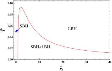
As shown in Fig. 6, the radius of the black hole horizon has a sudden change for a fixing phase transition temperature, which indicates that black hole microstructure gets a significant change. Now we define two new radii shifted by the critical value of the horizon radius at the phase transition

where $\tilde{r}_{\text{hs}}$ and $\tilde{r}_{\text{hl}}$ denote the horizon radius of the coexistence small and large black holes. We describe $\tilde{r}_{\text{h1}}$ and $\tilde{r}_{\text{h2}}$ in Fig. 7. From Fig. 7, we find that $\tilde{r}_{\text{h1}}$ has large values near $\tilde{T}$=0. Then it decreases with $\tilde{T}$. At the critical temperature, $\tilde{r}_{\text{h1}}$ vanishes for $\tilde{\alpha}$=0.4 and 1.4. Similar phenomena can also be observed for $\tilde{r}_{\text{h2}}$, see in Fig. 7. The only difference is that near $\tilde{T}$=0, $\tilde{r}_{\text{h2}}$ is finite. For example, $\tilde{r}_{\text{h2}}$=1.25 and 2.28 for $\tilde{\alpha}$=0.4 and 1.4, respectively. The reason is that $\tilde{r}_{\text{hl}}$ has no boundary, while $\tilde{r}_{\text{hs}}$ cannot be smaller than zero.

As shown above $\tilde{r}_{\text{h1}}$ and $\tilde{r}_{\text{h2}}$ vanish at the critical temperature, now, we aim to calculate its critical exponent. After the numerical calculation near $\tilde{T}$=0, we fit the data with the following form

where $a$ and $b$ are the fitting coefficients. We show the critical points and fitting coefficients in Table 1. Focusing on the coefficient $b$, we find that all them are near 1/2 with the relative deviation within 1.6%. Actually this value can also be obtained via expanding the equation of state of the system near the critical point. So we can conclude that $\tilde{r}_{\text{h1}}$ and $\tilde{r}_{\text{h2}}$ have a critical exponent 1/2. Hence $\tilde{r}_{h1,2}$, or the horizon radius, can serve as order parameters to characterize the small-large black hole phase transition. This also provides a fundamental interpretation of the horizon radius on investigating the dynamic process of the phase transitions.

As observed in Refs. Wei2020a ; Zhourun , the neutral GB-AdS black hole has an intriguing property that its interaction among the microscopic constituents maintains the same while its microstructure behaves different before and after the small-large black hole phase transition. In this subsection, we shall study the microstructure of the black hole in five dimensions and see whether this property holds for the charged case in the canonical ensemble.

Making use of the equation of state (28), we obtain the corresponding normalized scalar curvature of the Ruppeiner geometry via (27). When expressing in terms of $\tilde{T}$ and $\tilde{r}_{\text{h}}$, we have

Obviously, the charge is absent by using the reduced thermodynamic quantities. We plot $R_{\text{N}}$ for different $\tilde{T}$ and $\tilde{r}_{\text{h}}$ for $\tilde{\alpha}=0.4$ in Fig. 8. Other values of $\tilde{\alpha}$ share the similar pattern. For low temperature, $R_{\text{N}}$ has two negative divergences at two $\tilde{r}_{\text{h}}$. These two divergences merger at the critical point, and disappear beyond the critical temperature.

In order to show the details, we display $R_{\text{N}}$ for $\tilde{T}$=0.4$\tilde{T}_{\text{c}}$, 0.8$\tilde{T}_{\text{c}}$, $\tilde{T}_{\text{c}}$, and 1.2 $\tilde{T}_{\text{c}}$ in Fig. 9. It is clear that there are two negative divergent points for $\tilde{T}$=0.4$\tilde{T}_{\text{c}}$ and 0.8$\tilde{T}_{\text{c}}$, and one for $\tilde{T}=\tilde{T}_{\text{c}}$. While when $\tilde{T}=1.2\tilde{T}_{\text{c}}$, there is only a well with finite depth. More importantly, for $\tilde{T}$=0.4$\tilde{T}_{\text{c}}$ shown in Fig. 9, we find that there are two parameter regions, where $R_{\text{N}}$ is positive. One of them is at small $\tilde{r}_{\text{h}}$. For different temperatures, we always observe positive $R_{\text{N}}$. Another region is near $\tilde{r}_{\text{h}}$=2. However, it only appears for $\tilde{T}$=0.4$\tilde{T}_{\text{c}}$.

Now, we aim to uncover the divergent point and zero point of $R_{\text{N}}$. Solving (41), we obtain the divergent temperature $\tilde{T}_{\text{sp}}$ of $R_{\text{N}}$, which gives

Actually, the curve described by this temperature separates the metastable and unstable black hole branches, so we can call it the spinodal curve. The temperature corresponding to zero point is

Besides, at

$R_{\text{N}}$ will also vanish. We name the zero point curve of $R_{\text{N}}$ as the sign-changing point, across which $R_{\text{N}}$ changes its sign.

We describe these characteristic curves in the phase diagram in Fig. 10 for $\tilde{\alpha}$=0.4 and 1.4, respectively. The red solid curves are the coexistence curves of small and large black holes, below which is the coexistence regions, and the equation of state (28) may not hold. So we need to exclude such regions when we consider the normalized scalar curvature $R_{\text{N}}$, where we have used the equation of state in the calculation. The spinodal curves are marked in blue dashed lines. They only meet the coexistence curves at the critical points. The black dot-dashed lines are for the sign-changing curves, which separate the phase diagram into two regions, one with positive $R_{\text{N}}$ and another with negative $R_{\text{N}}$ shown in shadow regions.

For each $\tilde{\alpha}$, we find that there are three regions I, II, and III that have positive $R_{\text{N}}$, indicating that the repulsive interaction dominates among the black hole microstructure. While in other regions, the attractive interaction dominates. Since regions I and III are in the coexistence regions, we exclude them in our consideration. However, in region II, the small black holes with higher temperature always have positive $R_{\text{N}}$. So the repulsive interaction can be observed for the charged GB-AdS black holes. This behavior is quite similar to the charged AdS black hole without the GB coupling WeiWeiWei , while different from the neutral GB-AdS black holes Wei2020a ; Zhourun .

We also show the behaviors of $R_{\text{N}}$ along the coexistence small and large black hole curves for $\tilde{\alpha}$=0.4 and 1.4 in Fig 11. With the increase of the temperature, both the curves decrease, and go to negative infinity at the critical temperature. In particular, $R_{\text{N}}$ is positive at low temperature, $T<$0.062312 for $\tilde{\alpha}$=0.4 and $T<$0.028235 for $\tilde{\alpha}$=1.4 when it goes along the coexistence small black holes indicating that the repulsive interaction exists.

At the critical temperature, all these curves go to negative infinity. Here we plot $\ln|R_{\text{N}}|$ as a function of $\ln(\tilde{T}_{\text{c}}-\tilde{T})$ in Fig. 12 near the critical temperature. An intuitive impression is that it has a linear relation. We fit the data in the following form

The fitting coefficients are listed in Table 2. From the fitting results, we observe that the coefficient $\beta$ is much near -2 of relative deviation within $1\%$, which suggests

So $R_{\text{N}}$ has a critical exponent 2. Actually, this critical exponent can also be obtained by expanding the equation of state near the critical point.

In summary, we studied the thermodynamics and Ruppeiner geometry for the five-dimensional charged AdS black holes. Different from the neutral case, we observe that the repulsive interaction could exist for the small black hole with high temperature. Meanwhile, along the coexistence small or large black hole curve, $R_{\text{N}}$ takes different values indicating that the microscopic interaction changes among the black hole phase transition, where the microstructure changes either. The similar thing is that the normalized scalar curvature goes to negative infinity at the critical point, and it has a critical exponent 2.

References

- (1) D. Kastor, S. Ray, and J. Traschen, Enthalpy and the mechanics of AdS black holes, Class. Quant. Grav. 26, 195011 (2009), [arXiv:0904.2765[hep-th]].
- (2) A. Chamblin, R. Emparan, C. V. Johnson, and R. C. Myers, Charged AdS black holes and catastrophic holography, Phys. Rev. D 60, 064018 (1999), [arXiv:hep-th/9902170].
- (3) A. Chamblin, R. Emparan, C. V. Johnson, and R. C. Myers, Holography, thermodynamics and fluctuations of charged AdS black holes, Phys. Rev. D 60, 104026 (1999), [arXiv:hep-th/9904197].
- (4) M. M. Caldarelli, G. Cognola, and D. Klemm, Thermodynamics of Kerr-Newman-AdS Black Holes and Conformal Field Theories, Class. Quant. Grav. 17, 399 (2000), [arXiv:hep-th/9908022].
- (5) D. Kubiznak and R. B. Mann, - criticality of charged AdS black holes, J. High Energy Phys. 1207, 033 (2012), [arXiv:1205.0559[hep-th]].
- (6) N. Altamirano, D. Kubiznak, and R. B. Mann, Reentrant phase transitions in rotating ads black holes, Phys. Rev. D 88, 101502(R) (2013), [arXiv:1306.5756[hep-th]].
- (7) N. Altamirano, D. Kubiznak, R. B. Mann, and Z. Sherkatghanad, Kerr-AdS analogue of triple point and solid/liquid/gas phase transition, Class. Quant. Grav. 31, 042001 (2014), [arXiv:1308.2672[hep-th]].
- (8) N. Altamirano, D. Kubiznak, R. B. Mann, and Z. Sherkatghanad, Thermodynamics of rotating black holes and black rings: phase transitions and thermodynamic volume, Galaxies 2, 89 (2014), [arXiv:1401.2586[hep-th]].
- (9) B. P. Dolan, A. Kostouki, D. Kubiznak, and R. B. Mann, Isolated critical point from Lovelock gravity, Class. Quant. Grav. 31, 242001 (2014), [arXiv:1407.4783[hep-th]].
- (10) S.-W. Wei and Y.-X. Liu, Critical phenomena and thermodynamic geometry of charged Gauss-Bonnet AdS black holes, Phys. Rev. D 87, 044014 (2013), [arXiv:1209.1707[gr-qc]].
- (11) S.-W. Wei and Y.-X. Liu, Triple points and phase diagrams in the extended phase space of charged Gauss-Bonnet black holes in AdS space, Phys. Rev. D 90, 044057 (2014), [arXiv:1402.2837[hep-th]].
- (12) A. M. Frassino, D. Kubiznak, R. B. Mann, and F. Simovic, Multiple reentrant phase transitions and triple points in Lovelock thermodynamics, J. High Energy Phys. 1409, 080 (2014), [arXiv:1406.7015[hep-th]].
- (13) R.-G. Cai, L.-M. Cao, L. Li, and R.-Q. Yang, - criticality in the extended phase space of Gauss-Bonnet black holes in AdS space, J. High Energy Phys. 1309, 005 (2013), [arXiv:1306.6233[gr-qc]].
- (14) H. Xu, W. Xu, and L. Zhao, Extended phase space thermodynamics for third order Lovelock black holes in diverse dimensions, Eur. Phys. J. C 74, 3074 (2014), [arXiv:1405.4143[gr-qc]].
- (15) R. A. Hennigar, W. G. Brenna, and R. B. Mann, - criticality in quasitopological gravity, J. High Energy Phys. 1507, 077 (2015), [arXiv:1505.05517[hep-th]].
- (16) R. A. Hennigar and R. B. Mann, Reentrant phase transitions and van der Waals behaviour for hairy black holes, Entropy 17, 8056 (2015), [arXiv:1509.06798[hep-th]].
- (17) R. A. Hennigar, R. B. Mann, and E. Tjoa, Superfluid black holes, Phys. Rev. Lett. 118, 021301 (2017), [arXiv:1609.02564[hep-th]].
- (18) D.-C. Zou, R. Yue, and M. Zhang, Reentrant phase transitions of higher-dimensional AdS black holes in dRGT massive gravity, Eur. Phys. J. C 77, 256 (2017), [arXiv:1612.08056[gr-qc]].
- (19) S. W. Hawking, Particle creation by black holes, Commun. Math. Phys. 43, 199 (1975).
- (20) J. Bekenstein, Black holes and the second law, Lett. Nuovo Cim. 4, 737 (1972).
- (21) J. D. Bekenstein, Black holes and entropy, Phys. Rev. D 7, 2333 (1973).
- (22) J. M. Bardeen, B. Carter, and S. Hawking, The four laws of black hole mechanics, Commun. Math. Phys.31, 161 (1973).
- (23) G. Ruppeiner, Riemannian geometry in thermodynamic fluctuation theory, Rev. Mod. Phys. 67, 605 (1995); Erratum: Rev. Mod. Phys. 68, 313 (1996).
- (24) R.-G. Cai and J.-H. Cho, Thermodynamic curvature of the BTZ black hole, Phys. Rev. D 60, 067502 (1999).
- (25) S.-W. Wei and Y.-X. Liu, Insight into the microscopic structure of an AdS black hole from thermodynamical phase transition, Phys. Rev. Lett. 115, 111302 (2015), [arXiv:1502.00386[gr-qc]]; Erratum: Phys. Rev. Lett. 116, 169903 (2016).
- (26) S.-W. Wei, Y.-X. Liu, and R. B. Mann, Repulsive Interactions and Universal Properties of Charged AdS Black Hole Microstructures, Phys. Rev. Lett. 123, 071103 (2019), [arXiv:1906.10840[gr-qc]].
- (27) S.-W. Wei, Y.-X. Liu, and R. B. Mann, Ruppeiner Geometry, Phase Transitions, and the Microstructure of Charged AdS Black Holes, Phys. Rev. D 100, 124033 (2019) [arXiv:1909.03887[gr-qc]].
- (28) A. Dehyadegari, A. Sheykhi, and A. Montakhab, Critical behaviour and microscopic structure of charged AdS black holes via an alternative phase space, Phys. Lett. B 768, 235 (2017), [arXiv:1607.05333[gr-qc]].
- (29) M. K. Zangeneh, A. Dehyadegari, M. R. Mehdizadeh, B. Wang, and A. Sheykhi, Thermodynamics, phase transitions and Ruppeiner geometry for Einstein-dilaton Lifshitz black holes in the presence of Maxwell and Born-Infeld electrodynamics, Eur. Phys. J. C 77, 423 (2017), [arXiv:1610.06352[hep-th]].
- (30) M. Chabab, H. E. Moumni, S. Iraoui, K. Masmar, and S. Zhizeh, More insight into microscopic properties of RN-AdS black hole surrounded by quintessence via an alternative extended phase space, Int. J. Geom. Meth. Mod. Phys. 15, 1850171 (2018), [arXiv:1704.07720[gr-qc]].
- (31) Y.-G. Miao and Z.-M. Xu, Microscopic structures and thermal stability of black holes conformally coupled to scalar fields in five dimensions, Nucl. Phys. B 942, 205 (2019), [arXiv:1711.01757[hep-th]].
- (32) Y.-Z. Du, R. Zhao, and L.-C. Zhang, Microstructure and continuous phase transition of the gauss-bonnet ads black hole, Adv. High Energy Phys. 2020, 6395747 (2020), [arXiv:1901.07932[hep-th]].
- (33) Z.-M. Xu, B. Wu, and W.-L. Yang, The fine micro-thermal structures for the Reissner-Nordstrom black hole, Chin. Phys. C 44, 095106 (2020), [arXiv:1910.03378[gr-qc]].
- (34) A. Ghosh and C. Bhamidipati, Thermodynamic geometry for charged Gauss-Bonnet black holes in AdS spacetimes, Phys. Rev. D 101, 046005 (2020) [arXiv:1911.06280[gr-qc]].
- (35) A. N. Kumara, C. A. Rizwan, K. Hegde, and Ajith K. M, Repulsive Interactions in the Microstructure of Regular Hayward Black Hole in Anti-de Sitter Spacetime, Phys. Lett. B 807, 135556 (2020), [arXiv:2003.10175[gr-qc]].
- (36) P. K. Yerra and C. Bhamidipati, Ruppeiner Geometry, Phase Transitions and Microstructures of Black Holes in Massive Gravity, Int. J. Mod. Phys. A 35, 2050120 (2020), [arXiv:2006.07775[hep-th]].
- (37) B. Wu, C. Wang, Z.-M. Xu, and W.-L. Yang, Ruppeiner geometry and thermodynamic phase transition of the black hole in massive gravity, [arXiv:2006.09021[gr-qc]].
- (38) C. L. A. Rizwan, A. N. Kumara, K. Hegde, and D. Vaid, Coexistent Physics and Microstructure of the Regular Bardeen Black Hole in Anti-de Sitter Spacetime, Annals Phys. 422, 168320 (2020), [arXiv:2008.06472[gr-qc]].
- (39) A. N. Kumara, C.L. A. Rizwan, K. Hegde, M. S. Ali, and Ajith K.M, Ruppeiner Geometry, Reentrant Phase transition and Microstructure of Born-Infeld AdS Black Hole, Phys. Rev. D 103, 044025 (2021), [arXiv:2007.07861[gr-qc]].
- (40) S. A. H. Mansoori, M. Rafiee, and S.-W. Wei, Universal criticality of thermodynamic curvatures for charged AdS black holes, Phys. Rev. D 102, 124066 (2020), [arXiv:2007.03255[gr-qc]].
- (41) A. N. Kumara, C.L. A. Rizwan, K. Hegde, M. S. Ali, and Ajith K.M, Microstructure of five-dimensional neutral Gauss-Bonnet black hole in anti-de Sitter spacetime via - criticality, [arXiv:2006.13907[gr-qc]].
- (42) S.-W. Wei, Y.-X. Liu, and R. B. Mann, Novel dual relation and constant in Hawking-Page phase transition, Phys. Rev. D 102, 104011 (2020), [arXiv:2006.11503[gr-qc]].
- (43) A. Dehyadegari, A. Sheykhi, and S.-W. Wei, Microstructure of charged AdS black hole via - criticality, Phys. Rev. D 102, 104013 (2020), [arXiv:2006.12265[gr-qc]].
- (44) S.-W. Wei and Y.-X. Liu, Extended thermodynamics and microstructures of four-dimensional charged Gauss-Bonnet black hole in AdS space, Phys. Rev. D 101, 104018 (2020), [arXiv:2003.14275[gr-qc]].
- (45) S.-W. Wei and Y.-X. Liu, Intriguing microstructures of five-dimensional neutral Gauss-Bonnet AdS black hole, Phys. Lett. B 803, 135287 (2020), [arXiv:1910.04528[gr-qc]].
- (46) R. Zhou, Y.-X. Liu, and S.-W. Wei, Phase transition and microstructures of five-dimensional charged Gauss-Bonnet-AdS black holes in the grand canonical ensemble, Phys. Rev. D 102, 124015 (2020), [arXiv:2008.08301[gr-qc]].
- (47) Y.-P. Hu, L. Cai, X. Liang, and H. Zhang, Divergence Behavior of Thermodynamic Curvature Scalar at Critical Point in the extended Phase Space of generic Black Holes, [arXiv:2010.09363[gr-qc]].
- (48) Z.-M. Xu, Analytic phase structures and thermodynamic curvature for the charged AdS black hole in alternative phase space, Front. Phys. 16, 24502 (2021), [arXiv:2011.06736[gr-qc]].
- (49) J.-X. Mo and G.-Q. Li, Coexistence curves and molecule number densities of AdS black holes in the reduced parameter space, Phys. Rev. D 92, 024055 (2015), [arXiv:1604.07931[gr-qc]].
- (50) D. G. Boulware and S. Deser, String Generated Gravity Models, Phys. Rev. Lett. 55, 2656 (1985).
- (51) R. G. Cai, Gauss-Bonnet Black Holes in AdS Spaces, Phys. Rev. D 65, 084014 (2002), [arXiv:hep-th/0109133].
- (52) D. L. Wiltshire, Spherically Symmetric Solutions Of Einstein-maxwell Theory With A Gauss-bonnet Term, Phys. Lett. B 169, 36 (1986).
- (53) M. Cvetic, S. Nojiri, and S. D. Odintsov, Black Hole Thermodynamics and Negative Entropy in deSitter and Anti-deSitter Einstein-Gauss-Bonnet gravity, Nucl. Phys. B 628, 295 (2002), [arXiv:hep-th/0112045].
- (54) S.-W. Wei and Y.-X. Liu, Clapeyron equations and fitting formula of the coexistence curve in the extended phase space of charged AdS black holes, Phys. Rev. D 91, 044018 (2015), [arXiv:1411.5749[hep-th]].
- (55) S.-W. Wei, P. Cheng, and Y.-X. Liu, Analytical and exact critical phenomena of -dimensional singly spinning Kerr-AdS black holes, Phys. Rev. D 93, 084015 (2016), [arXiv:1510.00085[gr-qc]].