Temporal and spectral study of PKS 0208-512 during the 2019-2020 flare
Abstract
We present the temporal and spectral study of blazar PKS 0208-512, using recent flaring activity from November 2019 to May 2020, as detected by the Fermi-LAT observatory. The contemporaneous X-ray, optical/UV observations from Swift-XRT/UVOT are also used. During the activity state, 2-days binned -ray lightcurve shows multiple peaks indicating sub-flares. To understand the possible physical mechanisms behind flux enhancement, we divided the activity state of the source into several flux-states and carried out detailed temporal and spectral studies. Timing analysis of lightcurves suggest that peaks of sub-flares have rise and decay time on the order of days, with flux-doubling time 2-days. The 2-days binned -ray lightcurve shows double-lognormal flux distribution. The broadband spectral-energy-distribution (SED) for three selected flux states can be well fitted under synchrotron, synchrotron self-Compton (SSC) and external-Compton (EC) emission mechanisms. We obtained the physical parameters of the jet by the SED modeling and their confidence intervals through -statistics. Our SED modeling results suggest that during quiescent-state, -ray spectrum can be well explained by considering the EC-scattering of infra-red (IR) photons from dusty-torus. However, -ray spectra corresponding to flares demand additional target photons from broad-line-region (BLR) along with IR. These suggest that during flares, the emission-region is close to the edge of BLR, while for quiescent-state the emission-region is away from BLR. The best fit results suggest that marginal increase in magnetic-field during the flaring-episode can result in the flux enhancement. This is possibly associated with the efficiency of particle acceleration during flaring-states as compared to quiescent-state.
keywords:
galaxies: active – quasars: individual: PKS 0208-512 – galaxies: jets – radiation mechanisms: non-thermal– gamma-rays: galaxies.1 Introduction
Blazars are the class of active galactic nuclei (AGN) with relativistic jets pointing towards the observer within a few degrees (Urry &
Padovani 1995).
The jet emission is predominantly non-thermal in nature covering
the entire electromagnetic (EM) spectrum ranging from radio to very high energy -ray.
Their broadband spectral energy distribution (SED) is characterized by two prominent peaks, with the low energy peak generally observed between infrared (IR) to soft X-ray, while the high energy one falls at Mev/GeV energies. The low energy component is well explained by the synchrotron emission from relativistic electrons spiraling along the magnetic fields in the jet. The high energy component is generally modelled as the inverse-Compton (IC) scattering of low energy photons by the relativistic electrons. The source of low energy
target photons is either internal (synchrotron emission) or external (accretion disk, broad-line region, dusty torus, etc.) to the jet (Boettcher et al. 1997; Ghisellini &
Madau 1996; Błażejowski et al. 2000). Such a model is commonly referred as a leptonic model (Ghisellini &
Tavecchio 2009; Ghisellini et al. 2014). If the target photons for the inverse-Compton scattering is synchrotron photons itself
then the process is referred to as synchrotron self-Compton (SSC; Sikora et al. 2009). On the other hand, the scattering of external photons is known as external-Compton (EC; Dermer et al. 1992; Sikora
et al. 1994; Ghisellini et al. 1998) process.
One of the intriguing properties of blazars is that they show strong stochastic variability and occasional strong flares across the EM spectrum. The flux doubling time scale varies from minutes to several days (Paliya et al. 2015, Shukla & Mannheim 2020, Chatterjee et al. 2021). The rapid flux variability of the order of minutes/hours suggests the emission is produced from a region very close to the central engine (Ghisellini & Tavecchio 2008; Narayan & Piran 2012). In the past three decades, development in -ray astronomy has been an important tool to understand the spectral and temporal behavior of blazars (von Montigny et al. 1995; Abdo et al. 2010a; Abdo et al. 2010b; Madejski & Sikora 2016). Particularly, the launch of the Fermi-Large Area Telescope (LAT, Atwood et al. 2009) opened up a new window to study high energy -ray blazars. The recently updated Fermi-LAT catalog, 4FGL (Abdollahi et al. 2020) has more than five thousand -ray sources, 95% of which are blazars. A detailed study of the -ray blazars will help us to understand the acceleration and the dynamics of the underlying particle distribution. However, this also demands additional simultaneous broadband observation of the source in tandem with -rays. In the recent past, various telescopes i.e., the Neil Gehrels Swift observatory (Gehrels et al. 2004), Steward observatory (Smith et al. 2009), Owens Valley Radio Observatory (OVRO) 40-m (Richards et al. 2011) etc. operating at different energy ranges have been used to observe blazars along with Fermi-LAT. The simultaneous or quasi-simultaneous observations available from these instruments were collectively used to study the complex nature of blazars (Prince 2019; Prince et al. 2021; Shah et al. 2021).
The flat spectrum radio quasar (FSRQ) PKS 0208-512 is located at redshift z = 1.003 (Healey et al. 2008). The Parkes radio survey discovered the source (Bolton et al. 1964) and was observed regularly in -rays (Thompson et al. 1995) by EGRET onboard Compton Gamma-Ray Observatory (CGRO). The CGRO mission detected excess emission from PKS 0208-512 at soft -rays (1-3 MeV) during 1993 May-June. The -ray SED indicated a broad peak at MeV energies (Blom et al. 1995), later confirmed by INTEGRAL/SPI detection (Zhang et al. 2010). Henceforth, the source has been identified as ‘MeV blazar’.
PKS 0208-512 has been monitored regularly by the Fermi-LAT in a wide range 0.1-300 GeV and during October 2008 a moderate -ray flare was detected (Tosti 2008). The contemporaneous observations in optical/IR during this -ray flare, has been observed by SMARTS and ANDICAM (Buxton et al. 2008). Subsequently, several studies on the multiwavelength property of PKS 0208-512 have also been undertaken (Ghisellini et al. 2010; Zhang et al. 2010; Szostek 2011; Nesci et al. 2011; Blanchard et al. 2012; Chatterjee et al. 2013a; Chatterjee et al. 2013b).
From November, 2019 to May, 2020, PKS 0208-512 went through a major -ray flare and the follow-up ATel initiated a major coordinated observation of the source (Angioni 2019; Lucarelli et al. 2019; Angioni 2020; Angioni et al. 2020). The preliminary analysis of Fermi-LAT observations suggested that the daily averaged -ray flux at energy >100MeV enhanced up to 1.10.2 ph cm-2 s-1 on November 29, 2019, and 2.00.3 ph cm-2 s-1 on March 15, 2020 (Angioni, 2019, 2020). Further, AGILE observed the source during December 14-16, 2019 and using multi-source maximum likelihood analysis it measured a flux of 2.70.8 ph cm-2 s-1 for energy >100 MeV (Lucarelli et al. 2019).
The follow-up observations in the optical/UV and X-ray bands have been performed by Swift telescope under the Target of opportunity (ToO) program during December 17-24, 2019, and March 9-21, 2020. The rich simultaneous multi-wavelength observation of PKS 0208-512 during different flaring activity encouraged us to perform a detailed broadband timing and spectral study of the source. Our primary study is based on the -ray observation by Fermi-LAT and we supplement this with the simultaneous observation by Swift-XRT/UVOT in X-ray and optical/UV wavebands. The paper is organised as follows: In §2, we describe the multi-wavelength observations and data analysis procedure. In §3.1, we provide the broadband lightcurve and the identification of different flux states followed by the results obtained from the temporal and spectral analysis of -ray observations (§3.2 – §3.5). The results from Swift observations are given in §3.6. The detailed broadband spectral modeling of the source using synchrotron and inverse Compton emission processes is described in §4. Finally, the study results are discussed and summarized in §5. Throughout this work, we adopt a cosmology with , and km s-1 Mpc-1.
2 Observations and data analysis
2.1 Fermi-LAT
LAT (Atwood et al. 2009) is a -ray instrument onboard Fermi satellite launched by NASA in 2008 and sensitive in the energy range between 20 MeV to >300 GeV. It has a large field of view 2.4 sr and takes approximately 3 hours to scan the entire sky. The source PKS 0208-512, has been regularly monitored by Fermi-LAT. To study the long term -ray behavior of the source, we analyzed the data from September 4, 2017 to July 20, 2020 (MJD 58000-59050). This period includes both the low flux states as well as the high flux states of the source. The analysis has been carried out with the 10 degree region of interest (ROI) centered at the source position. We followed the standard analysis procedure described by the Fermi science tools 111https://fermi.gsfc.nasa.gov/ssc/data/analysis/documentation/ (version v10r0p5). The analysis was performed in the energy range from 100 MeV to 300 GeV with the evclass=128 and evtype=3, and a zenith angle cut >90∘ is applied to reduce the contamination from the Earth’s limb -rays. To generate the model xml file, we used the galactic diffuse emission model, “" and the isotropic background model, “". The model files are available publicly at the Fermi Science Support Center (FSSC). The spectral models and the spectral parameters for the sources in the ROI are defined in the fourth Fermi source catalog (4FGL; Abdollahi et al. 2020). To optimize the spectral parameters of the sources in the ROI, maximum Likelihood method is used and the detection of these sources were quantified by the test statistics (TS) 222To quantify the significance of the source, we used the Likelihood ratio test statistic (TS) defined as TS = 2 log(L1/L0), where L1 and L0 are the maximum Likelihood values for a model with and without the source in the specified location. The significance of the source detection is determined by TS(1/2) . The sources with TS < 9 (corresponds to 3; Mattox et al. 1996) have been removed for further analysis. The above procedure has been followed using the “unbinned likelihood analysis with python" developed by the Fermi collaboration.
The default spectral model of the source PKS 0208-512 is log parabola, the model parameters are optimized by the likelihood analysis. Finally, we fit the source spectrum integrated over the entire energy range 0.1-300 GeV during period (MJD 58000-59050) with a log-parabola function defined as
| (1) |
where, is the spectral slope at reference energy and is the peak spectral curvature. During the lightcurve generation, we freeze the parameters of all the sources except our source of interest PKS 0208-512, and 2-days binned -ray lightcurves for the flux and spectral parameters have been produced.
2.2 Swift-XRT
Swift is a space-based telescope also known as Neil Gehrels observatory, was launched in November 2004 to observe the transient phenomenon in the Universe (Gehrels et al. 2004). The instruments onboard Swift, used in our study are X-ray telescope (XRT, 0.3-10 keV), ultraviolet optical telescope (UVOT, 170-650 nm) with filters V, B, U for optical band and W1, M2, and W2 for UV band, respectively (Larionov et al. 2016). The source PKS 0208-512, has been observed regularly through the monitoring program and also by the target of opportunity (ToO) program. During the period MJD 58000-59050, Swift observed the source PKS 0208-512 in X-ray, optical, and UV as part of a ToO program only. The Swift ToO observations are follow-up of the -ray flaring activity of the source, reported on December 1, 2019 and March 16, 2020 (Angioni 2019, 2020). The follow-up Swift ToO observations were performed during December 17-24, 2019 (observation IDs : 00041512021, 00041512023, 00041512025, 00041512026, and 00041512027) and March 9-21, 2020 (observation IDs : 00035002131, 00035002132, 00035002133, 00035002134, and 00035002135). In total, we have 12 Swift observations of 1-2 ks each, for a total exposure time of 18.8 ks during the period from MJD 58669 to 58930. To reduce the X-ray data, we have followed the standard procedure. First, we ran the XRTPIPELINE to produce the clean event files, and to do that, the latest version of the calibration file (CALDB, version 20200305) is used. The cleaned event files for the photon counting (PC) mode were further used to create a source and background spectrum, using XSELECT.
To extract the source spectrum, a circular region of 20 arcsec is chosen around the source, while for the background spectrum, a circular region of 40 arcsec is selected far from the source to avoid contamination. In the case of pile-up affected observations with the source count rate above 0.5 ct/sec, an annular region of 4 arcsec inner radius and 20 arcsec outer radius were considered as the source region. The ancillary response files (ARF) and the redistribution matrix files (RMF) were generated using XRTMKARF from the Swift CALDB. For the flaring state, there are multiple observations in a given period and spectra from all these observations were combined using addspec333https://heasarc.gsfc.nasa.gov/ftools/caldb/help/addspec.txt. In addspec, RMF and ARF files for different observations were added with the source spectrum. The background spectra from different observations were added through mathpha444https://heasarc.gsfc.nasa.gov/ftools/caldb/help/mathpha.txt. Finally, the source spectrum and the background spectrum were combined through the tool grppha, and 20 counts in each bin have been considered. The resultant grouped spectrum was then added to the XSPEC for the modeling. We fit the X-ray spectrum corresponding to each ToO observation with an absorbed power-law model using XSPEC (Arnaud 1996), and estimate the flux and index. The Swift-XRT lightcurve is generated with each point corresponding to one observation. The X-ray spectrum obtained during the high and low state was used for the broadband SED modeling.
2.3 Swift-UVOT
Swift-UVOT (Roming et al. 2005) covers the optical and UV part of the spectrum with its three optical (U, B, V) and three UV (W1, M2, W2) filters. In case of multiple observations for a given period, we combined the images in the filters using the UVOTIMSUM tool. To extract the magnitudes from the images, the task UVOTSOURCE has been used with the source and background regions of 5 arcsec and 10 arcsec, respectively. The observed magnitudes were then corrected for the Galactic extinction, with E(B - V) = 0.0174 mag and the ratio AV /E(B - V ) = 3.1 from Schlafly & Finkbeiner (2011). We converted the magnitudes to flux units using the photometric zero-points from Breeveld et al. (2011) and the conversion factors from Larionov et al. (2016).
3 Results
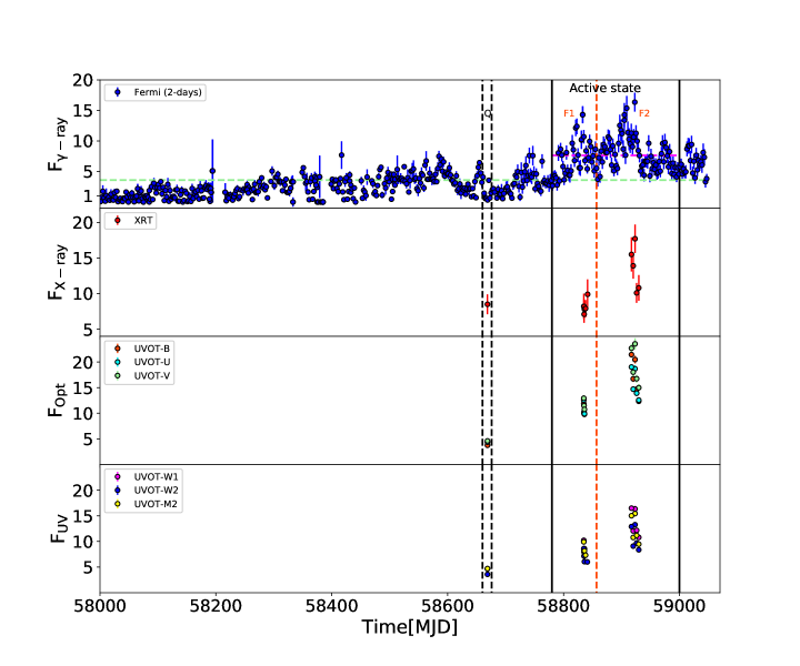
Fermi-LAT observation of PKS 0208-512 has shown enhanced flaring activity in -ray during the period 2019-2020 (Angioni, 2019, 2020). A daily averaged -ray flux (E>100MeV) of (1.10.2) ph cm-2 s-1 was reported for this source on November 29, 2019 (Angioni 2019). Subsequently, an increased flux with 2.00.3 ph cm-2 s-1 was observed on March 15, 2020, which is the highest daily binned -ray flux ever detected from this source (Angioni 2020). In the 2-days binned -ray lightcurve extending from September 4, 2017 to July 20, 2020 (MJD 58000-59050) and integrated over the energy range 100 MeV - 300 GeV, the peak flux (1.650.15) ph cm-2 s-1 is observed on March 15, 2020. This flux value is slightly lower than the daily binned flux reported by Angioni 2020. Moreover, we noted that 2-days binned -ray flux detected by Fermi-LAT is (1.430.14) ph cm-2 s-1 on December 16, 2019, which is lower than the 2-days integrated flux (2.70.8) ph cm-2 s-1 detected by AGILE on the same day. Such discrepancy in flux value can be possibly associated with the detection from different instruments and the analysis procedure. The maximum fluxes in X-ray, optical (B-band) and UV (W1-band), overlapping with the -ray lightcurve, are found to be (1.80.2) erg cm-2 s-1, (2.140.06) erg cm-2 s-1 and (1.650.05) erg cm-2 s-1 falling on March 9, 2020 as indicated by Swift-XRT/UVOT analysis. Here, we perform a detailed temporal and spectral study of the brightest -ray flare witnessed during MJD 58780-59000.
3.1 Multiwavelength lightcurves
The -ray lightcurve during the period from September 4, 2017 to July 20, 2020 (MJD 58000-59050), is shown in the top panel of Figure 1, where green dashed horizontal line corresponds to the average flux Fb = 3.60 ph cm-2 s-1, obtained from the 2-days binned data. The lightcurve in comparison with Fb suggests that the source was in a low flux state for a long period during September 4, 2017 to October 24, 2019 (MJD 58000-58780) with occasional minor outbursts. The state of enhanced -ray emission was observed from October 24, 2019 to May 31, 2020 (MJD 58780 - 59000), with the fluxes rising significantly above Fb. We consider this period as the ‘active state’ of the source and demarcate it with vertical black bold lines in Figure 1. During the -ray active state, two giant flares were identified with the first one peaking on December 16, 2019 (MJD 58833) with flux (1.430.14) ph cm-2 s-1 and the second one peaking on March 15, 2020 (MJD 58923) with flux (1.650.15) ph cm-2 s-1. The average flux during the active state is Fa = 7.6 ph cm-2 s-1 which is shown as dashed horizontal magenta line. Based on Fa, we divide the active region into two flaring states namely flare-1 (F1) and flare-2 (F2) with fluxes significantly higher than Fa. The peaks of these two flares are separated by 90 days. We have demarcated this division by red dashed vertical line in Figure 1. The second, third, and fourth panels from the top of Figure 1 correspond to X-ray, optical, and UV observations. It can be noted that the high flux points in X-ray, optical, and UV bands fall within the active state of -ray. Similarly, during -ray low flux state on July 4, 2019 (MJD 58668) we have single observation in other energy bands. The fluxes during this period are (6.642.64) ph cm-2 s-1 in -ray, (8.51.2) erg cm-2 s-1 in X-ray, (3.760.27) erg cm-2 s-1 in B-band, and (4.670.3) erg cm-2 s-1 in W1-band, respectively. Consistently, the flux values in X-ray, optical, and UV bands are minimal compared to ones observed during the -ray active state. We denote the -ray low flux state with simultaneous to X-ray, optical, and UV observations during the period from June to July, 2019 (MJD 58660 - 58676) as quiescent state ‘Q’ and represented by black dashed vertical lines.
3.2 -ray variability study
The variability behavior of the source can be quantified through fractional RMS variability amplitude, Fvar(Edelson et al. 2002) which is defined as the squared root of excess variance (). It accounts for the variability induced by the measurement uncertainties and its functional form can be represented as (Vaughan et al., 2003)
| (2) |
Here, F and err2 are the average flux and the mean square error in the observed flux, and the total variance of the observed lightcurve is denoted by S2. The error on Fvar can be estimated as (Vaughan et al., 2003)
| (3) |
where, N is the number of data points in the lightcurve. The fractional variability amplitude (Fvar) estimated during the period of June 26, 2019 to May 31, 2020 (MJD 58660 - 59000) is 0.720.01. This suggests the source showed a significantly high variability 72% in -ray and this is discussed further in §3.6.
To characterize the variability of the source in the flaring states, we estimate the variability time scales corresponding to F1 and F2 states. The flux doubling time during which the flux changes by a factor of two between consecutive time interval is expressed as (Zhang et al., 1999)
| (4) |
where, t1 and t2 are the two consecutive times with fluxes f1, and f2. The shortest variability time (tvar) then corresponds to the least value of estimated from all the consecutive time intervals from the entire lightcurve. We noted the fastest -ray variability time (tvar) during flare-1 state is, 2.0590.58 days with the flux values 2.780.89 and 8.041.29 () on November 2, 2019 (MJD 58789) and November 4, 2019 (MJD 58791). While for flare-2 state, it is found to be 2.590.79 days with the flux values 4.261.02 and 9.621.32 () measured during April 8, 2020 (MJD 58947) and April 10, 2020 (MJD 58949), respectively. The obtained tvar is close to the binning time, and this is discussed in §5.
The flux variability timescale can be used to constrain the size and the location of the emission region. Rapid variability observed in -ray indicates the size of the emission region to be of few Schwarzschild radius of the central black hole and hence should be located close to the central engine often within the broad-line region (BLR). However, the broadband spectral modelling of the FSRQs suggests the -ray emission can be well explained when the emission region is located outside the BLR (Sahayanathan & Godambe 2012; Shah et al. 2017). In this work, we found the fast variability timescale to be of the order of 2 days. This can be used to constrain the size of the emission region as R c t where, is the jet Doppler factor and c is the speed of light. For (Liodakis et al. 2017), R is estimated as 2.6 cm. Similarly, the distance of the emission region can be estimated as d 2 c tvar /(1+z) 5.2 cm (Abdo et al. 2011). These results are discussed in §5.
| States | MJD |
|---|---|
| 58780 - 58813 | |
| 58813 - 58840 | |
| 58840 - 58857 | |
| 58857 - 58888 | |
| 58888 - 58935 | |
| 58935 - 58963 | |
| 58963 - 59000 |
| States | F0.1-300GeV | Power Law | TS | TScurve | ||
| (10-7 ph cm-2 s-1) | ||||||
| 5.80.36 | -2.220.04 | – | – | 2386.37 | – | |
| 9.10.28 | -2.140.03 | – | – | 5353.15 | – | |
| 7.60.38 | -2.250.04 | – | – | 1915.97 | – | |
| 8.30.30 | -2.210.03 | – | – | 3996.26 | – | |
| 10.00.26 | -2.190.02 | – | – | 7112.10 | – | |
| 6.50.27 | -2.220.04 | – | – | 2599.61 | – | |
| 6.70.24 | -2.240.03 | – | – | 3636.70 | – | |
| Log-Parabola | ||||||
| 5.60.27 | 2.100.06 | 0.070.03 | – | 2396.46 | 10.09 | |
| 8.80.29 | 1.930.07 | 0.050.02 | – | 5369.20 | 16.05 | |
| 7.20.39 | 2.020.09 | 0.110.03 | – | 1928.65 | 12.68 | |
| 7.90.32 | 2.070.05 | 0.080.02 | – | 3993.41 | -2.85 | |
| 9.60.27 | 2.060.04 | 0.070.02 | – | 7143.33 | 31.23 | |
| 6.20.28 | 2.020.08 | 0.110.03 | – | 2620.01 | 20.40 | |
| 6.50.25 | 2.150.05 | 0.060.02 | – | 3656.53 | 19.83 | |
| Broken PowerLaw | Ebreak | |||||
| [GeV] | ||||||
| 5.70.27 | -2.140.06 | -2.390.09 | 1.010.21 | 2391.14 | 4.77 | |
| 8.80.29 | -2.040.04 | -2.320.07 | 0.910.14 | 5371.34 | 18.19 | |
| 7.30.39 | -2.080.07 | -2.690.19 | 1.020.37 | 1927.36 | 11.39 | |
| 8.00.47 | -2.060.08 | -2.530.13 | 1.020.18 | 3995.02 | -1.24 | |
| 9.70.26 | -2.080.04 | -2.470.08 | 1.030.18 | 7138.39 | 26.29 | |
| 6.20.28 | -2.040.07 | -2.620.16 | 0.990.35 | 2619.60 | 19.99 | |
| 6.50.25 | -2.130.06 | -2.440.11 | 0.860.47 | 3655.38 | 18.68 |
| Waveband | (MJD 58660 - 59000) |
|---|---|
| Fermi-LAT (0.1-300GeV) | |
| Swift-XRT (0.3-10keV) | |
| UVOT band-B | |
| UVOT band-U | |
| UVOT band-V | |
| UVOT band-W1 | |
| UVOT band-W2 | |
| UVOT band-M2 |
| States | Facilities | Obs-ID | Exposure (ks) |
|---|---|---|---|
| Q | Swift-XRT/UVOT | 00041512018 | 1.5 |
| F1b | Swift-XRT/UVOT | 00041512021 | 1.2 |
| Swift-XRT/UVOT | 00041512023 | 1.8 | |
| Swift-XRT/UVOT | 00041512025 | 1.6 | |
| Swift-XRT/UVOT | 00041512026 | 1.6 | |
| Swift-XRT/UVOT | 00041512027 | 1.1 | |
| F2b | Swift-XRT/UVOT | 00035002131 | 1.6 |
| Swift-XRT/UVOT | 00035002132 | 1.9 | |
| Swift-XRT/UVOT | 00035002133 | 1.9 | |
| Swift-XRT/UVOT | 00035002134 | 2.2 | |
| Swift-XRT/UVOT | 00035002135 | 1.2 |
| Parameters | Properties | |||||||||
|---|---|---|---|---|---|---|---|---|---|---|
| States | Seed | p1 | p2 | B | /dof | Pjet | Prad | |||
| photons | ||||||||||
| Q | IR | 13.93/12 | 14.79 | 45.69 | 43.69 | |||||
| F1b | IR + BLR | 11.97/15 | 13.40 | 45.61 | 44.05 | |||||
| F2b | IR + BLR | 19.54/16 | 11.67 | 45.20 | 44.43 |
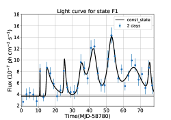

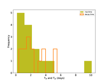
We also estimated the rise and decay times for the flares F1 and F2 using sum of exponentials of the form
| (5) |
where, TR and TD are the rise and decay time of a flare, F0 is the peak flux observed at time t0 and C is the constant introduced to obtain the base flux level. The temporal fit to the flares F1 and F2 indicated many sub flares which are shown in the upper panel of Figure 2. The reduced chi-square values to the fit of F1 and F2 flares are 0.91 and 1.42, respectively. The histogram of rise and decay time obtained through the temporal fit of the flares is shown in the lower panel of Figure 2. From the histogram, it is evident that most of the sub flares have rise time 1 day, and decay time 2 day. There are a few data points that show a sharp change in the flux value. Albeit the sharp changes are fitted by the sum of exponentials, the TR and TD values are not reliable and hence they are not included in the histogram.
3.3 -ray spectral variation
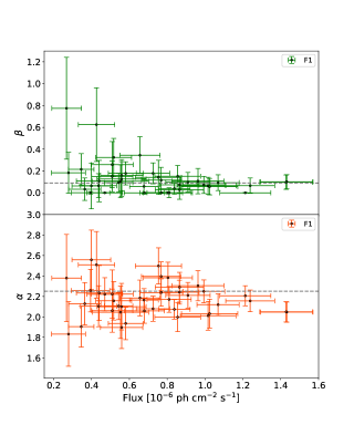
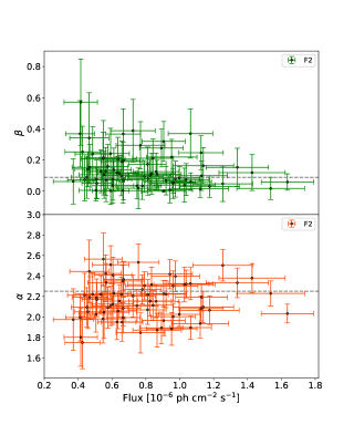
The -ray spectrum of PKS 0208-512 at the energy range 0.1-300 GeV is curved and better fitted by a log-parabola (4FGL; Abdollahi et al. 2020). To understand the spectral variation of the source during the active state, we performed a Spearman rank correlation study between the parameters defining the spectral shape and the 2-days integrated flux. In Figure 3, we showed the scatter plots between 2-days binned -ray flux (F0.1-300GeV) against the best fit log-parabola parameters and during the flaring states F1 (left side top and bottom plots) and F2 (right side top and bottom plots). For the flaring state F1, the Spearman’s rank correlation study between F0.1-300GeV and resulted in rank coefficient with null-hypothesis probability ; while between F0.1-300GeV and we get with . The high value of suggests the correlation results are inconclusive. Similarly, for the flaring state F2 the correlation study between F0.1-300GeV and resulted in with , and between F0.1-300GeV and we obtained with . The low value of P (<0.05) suggests there exists a mild negative correlation between F0.1-300GeV and during F2. Though ‘harder-when-brighter’ trend is generally witnessed in case of blazars, our correlation study was unable to confirm the same for the case of PKS 0208-512 (Shah et al., 2019; Khatoon et al., 2020; Prince, 2020; Prince et al., 2021). The ‘harder-when-brighter’ or ‘softer-when-brighter’ behavior can be interpreted as an outcome of shift in the Compton spectral peak when the peak falls in the energy range where Fermi-LAT is sensitive. For instance, a high energy shift in the Compton peak during a flare may result in ‘harder-when-brighter’ trend while low energy shift may imitate ‘softer-when-brighter’. However, since no such behavior is observed in our study, it is hard to conclude whether the spectral change is associated with the flux state of PKS 0208-512.
Furthermore, we added the default 4FGL and values i.e., 2.25 and 0.089 in Figure 3, as shown by the horizontal grey dashed lines. It can be seen in the Figure that during the states F1 and F2, most of the points are below the 4FGL value suggesting a harder spectral behavior compared to the 4FGL value. On the contrary, most of the points are marginally above the 4FGL value implying the spectrum is more curved during the flaring state compared to the 4FGL value.
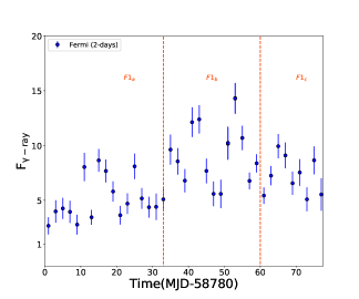
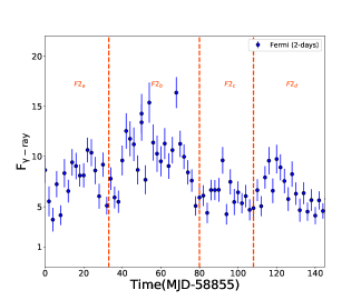
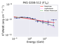
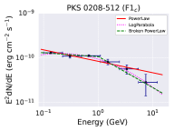
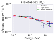
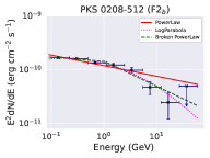
3.4 -ray spectral analysis
The flaring states F1 and F2, show multiple sub-flares as shown in Figure 4. To examine the spectral changes during these sub-flare states, we divided flare F1 into three sub-flares viz. F1a, F1b, and F1c (left plot of Figure 4), and the flare F2 into four sub-flares viz. F2a, F2b, F2c, and F2d (right plot of Figure 4), respectively. Each sub-flare shows rapid rise and decay patterns suggesting a strong flux variability. The time period corresponding to each sub-flare is reported in Table 1. For each sub-flare we generated the -ray spectra with the help of likesed.py code developed by the Fermi-LAT collaboration and available at Fermi science tools webpage555https://fermi.gsfc.nasa.gov/ssc/data/analysis/user/. We binned the entire energy range 0.1-300 GeV into nine equally spaced logarithmic energy bins. The -ray spectra made of nine data points are further fitted with the various spectral models: power law (PL), broken powerlaw (BPL), and log-parabola (LP)(see §2.1). These models are defined as
| (6) | |||||
| (7) | |||||
| (8) |
where, is the normalization, is the reference energy and is the break energy. The power-law indices are defined as , , and . The maximum log likelihood analysis is used to fit the -ray spectrum.
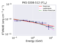
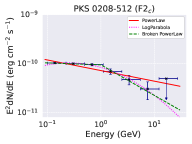
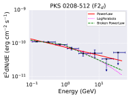
The fitted -ray spectrum for the sub-flares are shown in Figure 5 and their best fit parameters are presented in Table 2. Further, we estimated the test statistics of the curvature in the spectrum by calculating the parameter TScurve = 2 [log - log ], where is the likelihood function (Nolan et al. 2012). We consider curvature to be significant if TScurve 16 (equivalent to 4- level). It has been seen that the flaring states F1b, F2b, F2c, F2d exhibit significant curvature and/or breaks for the log-parabola and/or the broken power-law models. The TScurve values are reported in Table 2. The implications of these findings are discussed in §5.
3.5 Flux distribution of -ray lightcurve
Besides the spectral property, another striking feature of blazar lightcurve is the lognormal variability. The lognormal flux distribution has been observed in many blazars at various energy bands over different time scales (H.E.S.S. Collaboration et al. 2010; Chevalier et al. 2015; Sinha et al. 2016, 2017, 2018; Khatoon et al. 2020). The analysis of the flux distribution using Fermi-LAT lightcurves suggests that Fermi-blazars largely follow lognormal flux distribution (Ackermann et al. 2015; Shah et al. 2018; Romoli et al. 2018; Bhatta & Dhital 2020; Prince et al. 2021). The observed lognormal distribution in the blazar lightcurves can be interpreted as the result of a large collection of mini-jets which are randomly oriented inside the relativistic jet (Biteau & Giebels 2012). Alternatively, Sinha et al. (2018) showed that a Gaussian perturbation in the particle acceleration time-scale could also result in the lognormal flux distribution. Besides the single lognormal distribution, flux histograms of some blazars indicate double lognormal feature in different wavebands (Kushwaha et al. 2016; Shah et al. 2018; Khatoon et al. 2020). Kushwaha et al. (2016), observed that the source PKS 1510-089 has two lognormal profiles in the flux at near-infrared (NIR), optical, and -ray energies, and suggested that these two profiles are possibly connected to the two different flux states of the source. Further, Khatoon et al. (2020) found the double lognormal flux distribution at X-rays for the blazars Mrk 501 and Mrk 421, which can be a result of the double Gaussian distribution in the index.
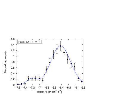
We studied the flux distribution of PKS 0208-512 using its -ray lightcurve. To ensure good statistics, we consider only the flux points for which > 2 and also with test statistic (TS) value > 9 (significance > 3). We use the Anderson Darling (AD) test statistic on the lightcurve where the null hypothesis checks if the sample is drawn from a normal distribution. The null hypothesis probability P < 0.01 would then indicate significant deviation from the normal distribution. Therefore, the P-values < 0.01 for the flux in linear-scale and log-scale would suggest the flux distribution is neither normal nor lognormal. We found the AD test statistics (r) and P-value for the flux in linear scale are 10.91 and ; while for the flux in logarithmic scale, the r-value and P-value are 3.25 and , respectively. This result suggests the flux distribution is neither normal nor lognormal. To explore this further, we construct the histogram of the logarithm of flux, which shows a double peak structure (Figure 7). We fitted the histogram with the double Gaussian probability density function (PDF) given by
| (9) |
Here, is the normalization fraction, and are the centroids of the distribution with widths and , respectively. We obtained the fit statistics /dof as 13.2/15 and this suggests the histogram of the logarithm of flux follows a double Gaussian PDF, which implies the flux distribution of the source is double log-normal. The best fit parameter values of , are -7.210.03, 0.140.03; , are -6.420.01, 0.270.01; with a value as 0.150.02, respectively. The double lognormal profile can be associated with two flux states of the source. Examining these flux states in detail demand precise study of the spectral evolution of the source. However, poor statistics do not let us to perform such a study at -rays and probably similar study at low energies have the potential to confirm this inference.
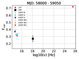
3.6 Study of Swift observations
Using the Swift observations shown in the second, third and fourth panels of Figure 1, we estimated the fractional variability Fvar (equation 2) in X-ray, optical, and UV bands during June, 2019 - May, 2020 (MJD 58660 - 59000). The Fvar values are depicted in Table 3 and in Figure 6 we plot Fvar against the photon frequency. The high Fvar values of optical/UV and -ray emissions than the X-ray emission may possibly be associated to the energy of relativistic electrons. The optical/UV and -ray emissions are due to the synchrotron and IC emission of high energy electrons respectively, while the X-ray emission is due to the IC emission of low energy tail of the electron distribution. This is evident from the broadband SED modeling of the source presented in §4. However, IC interpretation of the X-ray emission is also suggested for many FSRQs through broadband SED modelling (Chidiac et al., 2016; Rani et al., 2017; Shah et al., 2021).
4 Broadband spectral modelling
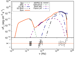
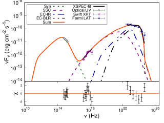
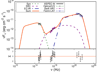
To perform the broadband SED modelling of the source PKS 0208-512 during different flux states, we selected three time segments including one quiescent state (Q state) MJD 58660 - 58676, and two flaring states with MJD 58813 - 58840 (F1b state) and MJD 58888 - 58935 (F2b state) from the lightcurve as shown in Figure 1. The selection was made such that each segment have simultaneous -ray, X-ray, UV and optical observations. The details of the Swift observations for states Q, F1b, and F2b are given in Table 4.
We carried the broadband SED modelling of the three selected states, using the one-zone leptonic model (Sahayanathan et al. 2018). In this model, we assume a scenario where the non-thermal emission from the blazar jet originates from a spherical blob of radius ‘R’ moving with a bulk Lorentz factor down the jet at an angle with respect to the observer’s direction. The emission region is permeated with the tangled magnetic field B, and populated by a broken power-law electron distribution described as
| (12) |
Here, K and are the normalization and the electron Lorentz factor, while the low and high energy power-law indices are denoted by p1 p2. The , are the minimum, and maximum Lorentz factors of the electron, and is the Lorentz factor corresponding to the break energy. The observed broadband emission from the source is modelled as synchrotron and inverse Compton (IC) emission by this electron distribution. The seed photons for the IC process are the synchrotron photons themselves (SSC) and the photon field external to the jet (EC). The source of external target photons considered for the SED modelling are the IR photons from the dusty torus (EC/IR) and the dominant Lyman-alpha line emission from the broad line region (EC/BLR). The emission from the dusty torus is assumed to be a black body with temperature T 1000K (Schartmann et al. 2005). For numerical simplicity, the line emission from BLR is modelled as a black body at T 42000 K (Peterson 2006). Since the final emissivity is estimated by convolving with a relatively broad particle distribution, this simplification will have a negligible effect on the resultant IC spectrum. The numerical model estimating the synchrotron and IC emissivity and the observed flux from the source parameters is added as a local model in XSPEC (Arnaud, 1996), to perform a statistical fit of the SED. The ASCII format of the optical, UV, X-ray, and -ray fluxes are converted to pha format using ftflx2xsp command and the fitting is performed using -statistics implimented in XSPEC.
The SED is mainly governed by the parameters: K, p1, p2, , B, R, , , temperature T and the fraction of the external target photons up scattered by the IC process. Clearly, the number of parameters exceeds the information available at four wavebands. Hence, to constrain the parameters, we enforce additional equipartition between particle and the magnetic field energy densities. The fitting is performed by first running the model on the observed SED to obtain acceptable residuals. Then the confidence intervals on parameters are obtained by freezing certain parameters to their best fit value. This is to avoid degeneracy introduced by the limited available observed information. Besides these, a 15 % error was evenly added to the data to get the reduced . This limit is demanded by XSPEC to obtain the confidence intervals on the fit parameters. The best fit model and the parameters corresponding to Q, F1b, and F2b are given in Figure 8 and Table 5. The parameters which are kept constant for all the epochs are the size of the emission region R = 2.44 cm (consistent with the observed variability time), viewing angle 2∘, the minimum and maximum values of particle Lorentz factor ( and ) = 50 and , and the energy density of the up scattered IR photon field as erg/cm3. On the other hand, the parameters p1, p2, , , and B are let to vary freely.
The -ray spectrum corresponding to the quiescent state can be readily explained by EC/IR mechanism alone; however, for the flaring states a combination of EC/IR and EC/BLR is required to fit the SED successfully. For the latter, the energy density of the up scattered BLR photons is set at erg/cm3. If the emission region is closer to the central black hole within BLR then the -ray spectrum will have the contribution from both EC/BLR and EC/IR. On the other hand, if the emission region is away from BLR but within the IR torus then EC/IR will be dominant. Therefore, our broadband spectral modelling suggests during the activity state the emission region is close to the central black hole than the quiescent state. This inference; however, may banks upon the assumptions (e.g. equipartition) imposed on the theoretical SED model and the choice of fixed parameters.
5 Summary and Discussions
The long-term monitoring of PKS 0208-512 by Fermi-LAT, together with the simultaneous observations in other wavebands by Swift, allow us to study the temporal and spectral behavior of the source in detail. The source showed an intense flaring activity during MJD 58780-59000. During this period, the source revealed two major outbursts, viz. F1 and F2. We obtained the fastest variability time-scale during F1 and F2 states as 2 days. However, using a 2-days binned lightcurve, the obtained variability time-scale of the order of 2-days may not be accurate. This may have an impact on the estimation of size and location of the emission region. Therefore, we generated the 1-day binned -ray lightcurve and estimated the fastest variability time of 0.950.35 day in F1-state, the corresponding values of R and d are obtained as 1.2 cm and 2.5 cm, respectively. These values do not deviate much from the values obtained from 2-days binned lightcurve and differ only by a factor of 2. Nevertheless, the larger error on the flux points in the 1-day binned lightcurve hinders us in locating the peaks of flares. Therefore, we considered the 2-days binned lightcurve in order to obtain the temporal characteristics of the source. Using 2-days variability time, the size and location of the -ray emission region are estimated as 2.6 cm and 5.2 cm, respectively. Considering a black hole of mass (Ghisellini et al. 2011), the derived emission region size is 2 order of magnitude larger than the Schwarzschild radius ( 3.0 cm). Relatively a longer time variability has been reported by using EGRET observations. For instance,von Montigny et al. 1995 found the variability time-scale of 8 days and this corresponds to the size of -ray emission as 3.2 cm for = 3.1. The authors considered a black hole of mass 1010 and the derived emission region size is 16 times larger than the Schwarzschild radii (1.9 cm). A variability time-scale of 4-days was also reported and this relates to the emission region of size 5 cm for (Stacy et al. 2008). However, the constraints obtained from the pair production opacity of the -rays suggest a lower limit on the Doppler factor as (Stacy et al. (2008)). A variability time of 4-days would then imply the distance of the emission region as, d 1.06 cm. For a disk luminosity Ld = 18 erg/sec (Ghisellini et al. 2011), the size of the BLR can be estimated as RBLR 4.24 cm. These results imply that the -rays are produced from a region close to the black hole. The multi-wavelength variability study between the fluxes in different wavebands suggests the variability is large in case of -rays and optical/UV compared to that of X-rays. This can be interpreted in terms of the electron energy responsible for the emission at these wavebands. The optical/UV emission corresponds to synchrotron emission from high energy electrons, whereas X-rays can be due to the IC emission from low energy electrons. Similarly, the -ray emission can be due to IC emission from high-energy electrons. This is also evident from the broadband SED modelling of the source.
The multiple peaks observed in the 2-days binned -ray flux lightcurve during states F1 and F2 are fitted with sum of exponentials. The result suggests that most of the peaks have characteristic rise and decay times of the order of 1-day. This finer sub-structures seen in -ray lightcurves of F1 and F2 are further divided as F1a, F1b, F1c, F2a, F2b, F2c, F2d. The -ray spectral study of these sub-flares modelled by the PL, LP, and BPL model shows that the states F1b, F2b, F2c, F2d revealed a significant curvature with TScurve values as 16.05, 31.23, 20.40, and 19.83, respectively. The observed curved spectrum is best fitted by the log-parabola (LP) and/or the broken power-law (BPL) functions. This also suggests significant curvature in the underlying electron distribution. Such curvatures in the electron distribution can be attributed to the energy dependence of the particle acceleration/escape time scales (Massaro et al. 2004; Jagan et al. 2018; Goswami et al. 2018). In Massaro et al. 2004, the authors showed that a curved particle distribution could originate when the acceleration probability is energy-dependent. The energy dependence of the escape timescale in the acceleration region can also be responsible for the curvature observed in the spectrum (Jagan et al. 2018; Goswami et al. 2018). Alternatively, EBL induced pair production absorption can also be a cause for curved -ray spectrum. However, we observed photons below 20 GeV in all the states and the EBL induced absorption optical depth for the redshift of PKS 0208-512 (z=1.003) at this -ray energies are very minimal (Franceschini et al. 2008). Hence it cannot account for the curvature observed in the -ray spectrum.
The broadband SED of PKS 0208-512 during different flux states have been fitted by a radiative model considering synchrotron, SSC, and EC processes. We find that the one-zone leptonic model can successfully explain the SED for all these three states. From the best fit parameters, it appears that no significant variation in the bulk Lorentz factor happened during different flux states, while a marginal decrease is noticed during the flare states. However, the observed information is not sufficient enough to constrain all the parameters and hence this conclusion cannot be treated as a robust one. Further, the values obtained are less compared to the typical value as observed in other FSRQs (Shah et al. 2017, 2019). Nevertheless, our broadband SED fitting suggests that the -ray spectra during flaring (F1b F2b) states demand the EC scattering of photons from both BLR and dusty torus. On the other hand, for the quiescent (Q) state, EC scattering of IR photons alone is capable to explain the -ray spectrum. This result can be interpreted in terms of the location of the emission region during different activity states. For instance, during F1b and F2b states, the emission region is well within BLR and hence the photons from BLR as well as IR torus will be upscattered through EC process. While in the case of Q state, the emission region may lie ahead of the BLR. From Table 5, it appears decreases marginally during the flare states. This may appear to contradict to our inference since the emission region is closer to the central black hole during active states and it is expected the to be larger. However, within the estimated confidence intervals we do not find any significant change in . Additionally, any deviation from the equipartition during the flaring state can also modify significantly. The flare state is also associated with a marginal increase in magnetic field and the particle energy density (through equipartition). This maybe associated with efficient particle acceleration during the flaring states as compared to the quiescent state. This is also consistent with the change in power-law index (p1) of the particle distribution where it hardens during the flaring states. Non-availability of sufficiently high energy spectra (which can probe the high energy tail electron distribution) do not let us to obtain the upper bound of p2. However, its quite evident the difference between p1 and p2 is larger than 1/2 and hence the origin of the broken power-law may not be strictly associated with the radiative cooling interpretation of a power-law electron distribution (Kardashev 1962).
For MeV blazars, X-rays can be due to the EC mechanism as well (in the framework of leptonic model, see e.g. Ghisellini & Tavecchio 2009; Sbarrato et al. 2015; Ajello et al. 2016; Marcotulli et al. 2020). However, Chatterjee et al. 2013b has performed the broadband study of PKS 0208-512 using one-zone leptonic model, where the optical, X-ray, and -ray emissions can be explained by the synchrotron, SSC, and EC processes. Further, explanation of X-ray emission of FSRQs through EC process demand a significant deviation from the equipartition (Sahayanathan & Godambe 2012; Shah et al. 2017). In the present work also, we find that the SSC and EC interpretation of the X-ray and -ray emission from PKS 0208-512 do not require any deviation from the equipartition condition. The optical/UV/X-ray observation period considered for the broadband SED modelling does not encompass the selected -ray period fully. However, we believe the average flux obtained during this period do not change the parameters obtained from the broadband fitting significantly unless extreme low/high optical/UV/X-ray fluxes are missed in the time gap. Alternatively, reducing the -ray observation period consistent with the optical/UV/X-ray observation will not deviate the average -ray flux significantly. On the other hand, this may impact in poor statistics due to less number of -ray photons. Hence, the physical parameters obtained through this study largely define the source within the ambit of the model assumptions. Future observations at very high energy by upcoming experiment Cherenkov Telescope Array (CTA Consortium & Ong 2019) have a better potential to relax some of the underlying assumptions and gain better constraint on the physical parameters.
Acknowledgements
We thank the anonymous referee for valuable comments and suggestions. We acknowledge the use of -ray data, software obtained from Fermi Science Support Center (FSSC), and the Swift-XRT/UVOT data from NASA’s High Energy Astrophysics Science Archive Research Center (HEASARC), service of Goddard Space Flight Center. This work has made use of the XRT Data Analysis Software (XRTDAS) developed under the responsibility of the ASI Science Data Center (ASDC), Italy. R.K. and R.G. would like to thank CSIR, New Delhi (03(1412)/17/EMR-II) for financial support. R.P. acknowledges the support by the Polish Funding Agency National Science Centre, project 2017/26/A/ST9/00756 (MAESTRO 9), and MNiSW grant DIR/WK/2018/12. Z.S. is supported by the Department of Science and Technology, Government of India, under the INSPIRE Faculty grant (DST/INSPIRE/04/2020/002319).
Data Availability
The data and software used in this research are available at Fermi Science Support Center (FSSC), NASA’s HEASARC webpages with the links given in the manuscript.
References
- Abdo et al. (2010a) Abdo A. A., et al., 2010a, The Astrophysical Journal, 710, 1271
- Abdo et al. (2010b) Abdo A. A., et al., 2010b, ApJ, 722, 520
- Abdo et al. (2011) Abdo A. A., et al., 2011, ApJ, 733, L26
- Abdollahi et al. (2020) Abdollahi S., et al., 2020, ApJS, 247, 33
- Ackermann et al. (2015) Ackermann M., et al., 2015, The Astrophysical Journal, 810, 14
- Ajello et al. (2016) Ajello M., et al., 2016, ApJ, 826, 76
- Angioni (2019) Angioni R., 2019, The Astronomer’s Telegram, 13320, 1
- Angioni (2020) Angioni R., 2020, The Astronomer’s Telegram, 13558, 1
- Angioni et al. (2020) Angioni R., Ciprini S., Yusafzai A., 2020, The Astronomer’s Telegram, 13847, 1
- Arnaud (1996) Arnaud K. A., 1996, in Jacoby G. H., Barnes J., eds, Astronomical Society of the Pacific Conference Series Vol. 101, Astronomical Data Analysis Software and Systems V. p. 17
- Atwood et al. (2009) Atwood W. B., et al., 2009, ApJ, 697, 1071
- Bhatta & Dhital (2020) Bhatta G., Dhital N., 2020, ApJ, 891, 120
- Biteau & Giebels (2012) Biteau J., Giebels B., 2012, A&A, 548, A123
- Blanchard et al. (2012) Blanchard J. M., et al., 2012, arXiv e-prints, p. arXiv:1202.4499
- Błażejowski et al. (2000) Błażejowski M., Sikora M., Moderski R., Madejski G. M., 2000, ApJ, 545, 107
- Blom et al. (1995) Blom J. J., et al., 1995, A&A, 298, L33
- Boettcher et al. (1997) Boettcher M., Mause H., Schlickeiser R., 1997, A&A, 324, 395
- Bolton et al. (1964) Bolton J. G., Gardner F. F., Mackey M. B., 1964, Australian Journal of Physics, 17, 340
- Breeveld et al. (2011) Breeveld A. A., Landsman W., Holland S. T., Roming P., Kuin N. P. M., Page M. J., 2011, in McEnery J. E., Racusin J. L., Gehrels N., eds, American Institute of Physics Conference Series Vol. 1358, American Institute of Physics Conference Series. pp 373–376 (arXiv:1102.4717), doi:10.1063/1.3621807
- Buxton et al. (2008) Buxton M., Bailyn C., Coppi P., Kaptur A., Isler J., Urry M., Maraschi L., Fossati G., 2008, The Astronomer’s Telegram, 1751, 1
- CTA Consortium & Ong (2019) CTA Consortium Ong R. A., 2019, in European Physical Journal Web of Conferences. p. 01038 (arXiv:1904.12196), doi:10.1051/epjconf/201920901038
- Chatterjee et al. (2013a) Chatterjee R., et al., 2013a, ApJ, 763, L11
- Chatterjee et al. (2013b) Chatterjee R., Nalewajko K., Myers A. D., 2013b, ApJ, 771, L25
- Chatterjee et al. (2021) Chatterjee R., et al., 2021, Journal of Astrophysics and Astronomy, 42, 80
- Chevalier et al. (2015) Chevalier J., Kastendieck M. A., Rieger F. M., Maurin G., Lenain J. P., Lamanna G., 2015, in 34th International Cosmic Ray Conference (ICRC2015). p. 829
- Chidiac et al. (2016) Chidiac C., et al., 2016, A&A, 590, A61
- Dermer et al. (1992) Dermer C. D., Schlickeiser R., Mastichiadis A., 1992, A&A, 256, L27
- Edelson et al. (2002) Edelson R., Turner T. J., Pounds K., Vaughan S., Markowitz A., Marshall H., Dobbie P., Warwick R., 2002, The Astrophysical Journal, 568, 610
- Franceschini et al. (2008) Franceschini A., Rodighiero G., Vaccari M., 2008, A&A, 487, 837
- Gehrels et al. (2004) Gehrels N., et al., 2004, ApJ, 611, 1005
- Ghisellini & Madau (1996) Ghisellini G., Madau P., 1996, MNRAS, 280, 67
- Ghisellini & Tavecchio (2008) Ghisellini G., Tavecchio F., 2008, MNRAS, 386, L28
- Ghisellini & Tavecchio (2009) Ghisellini G., Tavecchio F., 2009, MNRAS, 397, 985
- Ghisellini et al. (1998) Ghisellini G., Celotti A., Fossati G., Maraschi L., Comastri A., 1998, Monthly Notices of the Royal Astronomical Society, 301, 451
- Ghisellini et al. (2010) Ghisellini G., Tavecchio F., Foschini L., Ghirlanda G., Maraschi L., Celotti A., 2010, MNRAS, 402, 497
- Ghisellini et al. (2011) Ghisellini G., Tavecchio F., Foschini L., Ghirlanda G., 2011, MNRAS, 414, 2674
- Ghisellini et al. (2014) Ghisellini G., Tavecchio F., Maraschi L., Celotti A., Sbarrato T., 2014, Nature, 515, 376
- Goswami et al. (2018) Goswami P., Sahayanathan S., Sinha A., Misra R., Gogoi R., 2018, MNRAS, 480, 2046
- H.E.S.S. Collaboration et al. (2010) H.E.S.S. Collaboration et al., 2010, A&A, 520, A83
- Healey et al. (2008) Healey S. E., et al., 2008, ApJS, 175, 97
- Jagan et al. (2018) Jagan S. K., Sahayanathan S., Misra R., Ravikumar C. D., Jeena K., 2018, MNRAS, 478, L105
- Kardashev (1962) Kardashev N. S., 1962, Soviet Ast., 6, 317
- Khatoon et al. (2020) Khatoon R., Shah Z., Misra R., Gogoi R., 2020, MNRAS, 491, 1934
- Kushwaha et al. (2016) Kushwaha P., Chandra S., Misra R., Sahayanathan S., Singh K. P., Baliyan K. S., 2016, ApJ, 822, L13
- Larionov et al. (2016) Larionov V. M., et al., 2016, Monthly Notices of the Royal Astronomical Society, 461, 3047
- Liodakis et al. (2017) Liodakis I., et al., 2017, MNRAS, 466, 4625
- Lucarelli et al. (2019) Lucarelli F., et al., 2019, The Astronomer’s Telegram, 13352, 1
- Madejski & Sikora (2016) Madejski G. G., Sikora M., 2016, ARA&A, 54, 725
- Marcotulli et al. (2020) Marcotulli L., et al., 2020, ApJ, 889, 164
- Massaro et al. (2004) Massaro E., Perri M., Giommi P., Nesci R., 2004, A&A, 413, 489
- Mattox et al. (1996) Mattox J. R., et al., 1996, ApJ, 461, 396
- Narayan & Piran (2012) Narayan R., Piran T., 2012, MNRAS, 420, 604
- Nesci et al. (2011) Nesci R., Kadler M., Ojha R., Pursimo T., Tosti G., Blanchard J., Lovell J., 2011, The Astronomer’s Telegram, 3421, 1
- Nolan et al. (2012) Nolan P. L., et al., 2012, ApJS, 199, 31
- Paliya et al. (2015) Paliya V. S., Böttcher M., Diltz C., Stalin C. S., Sahayanathan S., Ravikumar C. D., 2015, The Astrophysical Journal, 811, 143
- Peterson (2006) Peterson B. M., 2006, The Broad-Line Region in Active Galactic Nuclei. p. 77, doi:10.1007/3-540-34621-X_3
- Prince (2019) Prince R., 2019, ApJ, 871, 101
- Prince (2020) Prince R., 2020, ApJ, 890, 164
- Prince et al. (2021) Prince R., Khatoon R., Stalin C. S., 2021, MNRAS, 502, 5245
- Rani et al. (2017) Rani B., Krichbaum T. P., Lee S. S., Sokolovsky K., Kang S., Byun D. Y., Mosunova D., Zensus J. A., 2017, MNRAS, 464, 418
- Richards et al. (2011) Richards J. L., et al., 2011, The Astrophysical Journal Supplement Series, 194, 29
- Roming et al. (2005) Roming P. W. A., et al., 2005, Space Sci. Rev., 120, 95
- Romoli et al. (2018) Romoli C., Chakraborty N., Dorner D., Taylor A., Blank M., 2018, Galaxies, 6, 135
- Sahayanathan & Godambe (2012) Sahayanathan S., Godambe S., 2012, MNRAS, 419, 1660
- Sahayanathan et al. (2018) Sahayanathan S., Sinha A., Misra R., 2018, Research in Astronomy and Astrophysics, 18, 035
- Sbarrato et al. (2015) Sbarrato T., Ghisellini G., Tagliaferri G., Foschini L., Nardini M., Tavecchio F., Gehrels N., 2015, MNRAS, 446, 2483
- Schartmann et al. (2005) Schartmann M., Meisenheimer K., Camenzind M., Wolf S., Henning T., 2005, A&A, 437, 861
- Schlafly & Finkbeiner (2011) Schlafly E. F., Finkbeiner D. P., 2011, ApJ, 737, 103
- Shah et al. (2017) Shah Z., Sahayanathan S., Mankuzhiyil N., Kushwaha P., Misra R., Iqbal N., 2017, MNRAS, 470, 3283
- Shah et al. (2018) Shah Z., Mankuzhiyil N., Sinha A., Misra R., Sahayanathan S., Iqbal N., 2018, Research in Astronomy and Astrophysics, 18, 141
- Shah et al. (2019) Shah Z., Jithesh V., Sahayanathan S., Misra R., Iqbal N., 2019, MNRAS, 484, 3168
- Shah et al. (2021) Shah Z., Jithesh V., Sahayanathan S., Iqbal N., 2021, MNRAS,
- Shukla & Mannheim (2020) Shukla A., Mannheim K., 2020, Nature Communications, 11, 4176
- Sikora et al. (1994) Sikora M., Begelman M. C., Rees M. J., 1994, ApJ, 421, 153
- Sikora et al. (2009) Sikora M., Stawarz Ł., Moderski R., Nalewajko K., Madejski G. M., 2009, ApJ, 704, 38
- Sinha et al. (2016) Sinha A., et al., 2016, A&A, 591, A83
- Sinha et al. (2017) Sinha A., Sahayanathan S., Acharya B. S., Anupama G. C., Chitnis V. R., Singh B. B., 2017, ApJ, 836, 83
- Sinha et al. (2018) Sinha A., Khatoon R., Misra R., Sahayanathan S., Mandal S., Gogoi R., Bhatt N., 2018, MNRAS, 480, L116
- Smith et al. (2009) Smith P. S., Montiel E., Rightley S., Turner J., Schmidt G. D., Jannuzi B. T., 2009, arXiv e-prints, p. arXiv:0912.3621
- Stacy et al. (2008) Stacy J., Vestrand W., Sreekumar P., 2008, The Astrophysical Journal, 598, 216
- Szostek (2011) Szostek A., 2011, The Astronomer’s Telegram, 3338, 1
- Thompson et al. (1995) Thompson D. J., et al., 1995, ApJS, 101, 259
- Tosti (2008) Tosti G., 2008, The Astronomer’s Telegram, 1759, 1
- Urry & Padovani (1995) Urry C. M., Padovani P., 1995, PASP, 107, 803
- Vaughan et al. (2003) Vaughan S., Edelson R., Warwick R. S., Uttley P., 2003, MNRAS, 345, 1271
- Zhang et al. (1999) Zhang Y. H., et al., 1999, ApJ, 527, 719
- Zhang et al. (2010) Zhang S., Collmar W., Torres D. F., Wang J. M., Lang M., Zhang S. N., 2010, A&A, 514, A69
- von Montigny et al. (1995) von Montigny C., et al., 1995, ApJ, 440, 525