capbtabboxtable[][\FBwidth]
TAX-Pose: Task-Specific Cross-Pose Estimation
for Robot Manipulation - Supplement
Appendix A Translational Equivariance
One benefit of our method is that it is translationally equivariant by construction. This mean that if the object point clouds, and , are translated by random translation and , respectively, i.e. and , then the resulting corrected virtual correspondences, and , respectively, are transformed accordingly, i.e. and , respectively, as we will show below. This results in an estimated cross-pose transformation that is also equivariant to translation by construction.
This is achieved because our learned features and correspondence residuals are invariant to translation, and our virtual correspondence points are equivariant to translation.
First, our point features are a function of centered point clouds. That is, given point clouds and , the mean of each point cloud is computed as
This mean is then subtracted from the clouds,
which centers the cloud at the origin. The features are then computed on the centered point clouds:
Since the point clouds are centered before features are computed, the features are invariant to an arbitrary translation .
These translationally invariant features are then used, along with the original point clouds, to compute “corrected virtual points” as a combination of virtual correspondence points, and the correspondence residuals, . As we will see below, the “corrected virtual points” will be translationally equivariant by construction.
The virtual correspondence points, , are computed using weights that are a function of only the translationally invariant features, :
thus the weights are also translationally invariant. These translationally invariant weights are applied to the translated cloud
since . Thus the virtual correspondence points are equivalently translated. The same logic follows for the virtual correspondence points . This gives us a set of translationally equivaraint virtual correspondence points and .
The correspondence residuals, , are a direct function of only the translationally invariant features ,
therefore they are also translationally invariant.
Since the virtual correspondence points are translationally equivariant, and the correspondence residuals are translationally invariant, , the final corrected virtual correspondence points, , are translationally equivariant, i.e. . This also holds for , giving us the final translationally equivariant correspondences between the translated object clouds as and , where .
As a result, the final computed transformation will be automatically adjusted accordingly. Given that we use weighted SVD to compute the optimal transform, , with rotational component and translational component , the optimal rotation remains unchanged if the point cloud is translated, , since the rotation is computed as a function of the centered point clouds. The optimal translation is defined as
where and are the means of the corrected virtual correspondence points, , and the object cloud , respectively, for object . Therefore, the optimal translation between the translated point cloud and corrected virtual correspondence points is
{align*}
t_A’ B’ &= ¯~v_A’ - R_AB ⋅¯p_A’
= ¯~v_A + t_β- R_AB ⋅(¯p_A + t_α)
= ¯~v_A + t_β- R_AB ⋅¯p_A - R_AB ⋅t_α
= t_AB + t_β- R_AB ⋅t_α
To simplify the analysis, if we assume that, for a given example, , then we get , demonstrating that the computed transformation is translation-equivariant by construction.
Appendix B Weighted SVD
The objective function for computing the optimal rotation and translation given a set of correspondences for object , and weights , is as follows:
First we center (denoted with ) the point clouds and virtual points independently, with respect to the learned weights, and stack them into frame-specific matrices (along with weights) retaining their relative position and correspondence:
Then the minimizing rotation is given by:
| (1) |
| (2) |
where and is a differentiable SVD operation [papadopoulo2000estimating].
The optimal translation can be computed as:
| (3) |
with . In the special translation-only case, the optimal translation and be computed by setting to identity in above equations. The final transform can be assembled:
| (4) |
Appendix C Cross-Object Attention Weight Computation
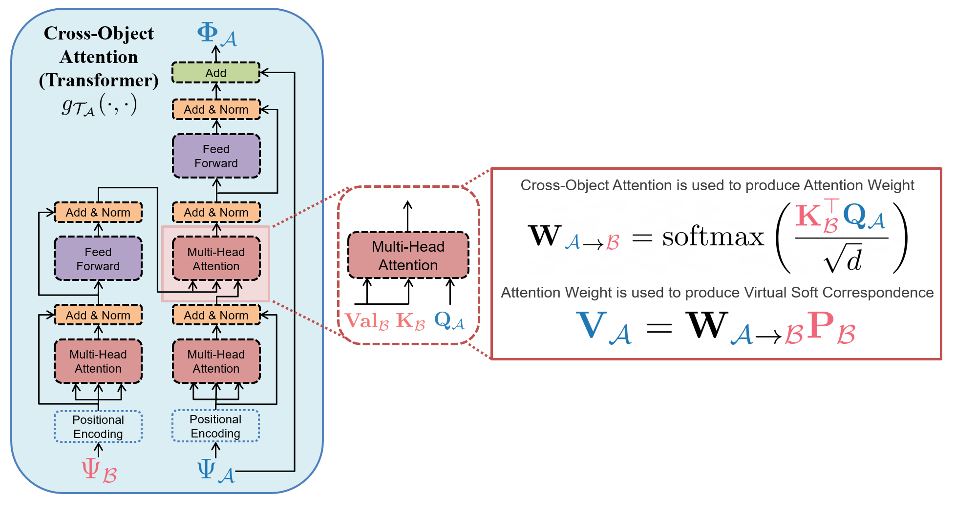
To map our estimated features we obtain from an object-specific Embedding Network (DGCNN), and for object , respectively, to a set of normalized weight vectors and , we use the cross attention mechanism of our Transformer module [vaswani2017attention]. Following Equations 5a and 5b from the paper, we can extract the desired normalized weight vector for any point using the intermediate attention embeddings of cross-object attention module as:
| (5) |
where , and are the query and key (respectively) for object associated with cross-object attention Transformer module , as shown in Figure S.1. These weights are then used to compute the virtual corresponding points , using Equations 5a and 5b in the main paper.
C.1 Ablation
To explore the importance of this weight computation design choice described in Equation 5, we conducted an ablation experiment on this design choice against an alternative, arguably simpler method for cross-object attention weight computation that was used in prior work) [wang2019deep]. Since the point embeddings and have the same dimension , we can select the inner product of the space as a similarity metric between two embeddings. For any point , we can extract the desired normalized weight vector with the softmax function:
| (6) |
This is the approach used in the prior work of Deep Closest Point (DCP) [wang2019deep]. In the experiments below, we refer to this approach as point embedding dot-product.
We conducted an ablation experiment on the weight computation method used in TAX-Pose (Equation 5) against the simpler approach from DCP [wang2019deep] (Equation 6), on the upright mug hanging task in simulation. The models are trained from 10 demonstrations and tested on 100 trials over the test mug set. As seen in Table LABEL:tab:ablation_weight, the TAX-Pose approach (Equation 5) outperforms point embedding dot-product (Equation 6) in all three evaluation categories on grasp, place, and overall in terms of test success rate.
Appendix D Supervision Details
To train the encoders , as well as the residual networks , , we use a set of losses defined below. We assume we have access to a set of demonstrations of the task, in which the action and anchor objects are in the target relative pose such that .
Point Displacement Loss [xiang2017posecnn, li2018deepim]: Instead of directly supervising the rotation and translation (as is done in DCP), we supervise the predicted transformation using its effect on the points. For this loss, we take the point clouds of the objects in the demonstration configuration, and transform each cloud by a random transform, , and . This would give us a ground truth transform of ; the inverse of this transform would move object to the correct position relative to object . Using this ground truth transform, we compute the MSE loss between the correctly transformed points and the points transformed using our prediction.
| (7) |
Direct Correspondence Loss. While the Point Displacement Loss best describes errors seen at inference time, it can lead to correspondences that are inaccurate but whose errors average to the correct pose. To improve these errors we directly supervise the learned correspondences and :
| (8) |
Correspondence Consistency Loss. Furthermore, a consistency loss can be used. This loss penalizes correspondences that deviate from the final predicted transform. A benefit of this loss is that it can help the network learn to respect the rigidity of the object, while it is still learning to accurately place the object. Note, that this is similar to the Direct Correspondence Loss, but uses the predicted transform as opposed to the ground truth one. As such, this loss requires no ground truth:
| (9) |
Overall Training Procedure. We train with a combined loss , where and are hyperparameters. We use a similar network architecture as DCP [wang2019deep], which consists of DGCNN [wang2019dynamic] and a Transformer [vaswani2017attention]. We also optionally incorporate a contextual embedding vector into each DGCNN module - identical to the contextual encoding proposed in the original DGCNN paper - which can be used to provide an embedding of the specific placement relationship that is desired in a scene (e.g. selecting a “top” vs. “left” placement position) and thus enable goal conditioned placement. We refer to this variant as TAX-Pose GC (goal-conditioned). We briefly experimented with Vector Neurons [deng2021vector] and found that this led to worse performance on this task. In order to quickly adapt to new tasks, we optionally pre-train the DGCNN embedding networks over a large set of individual objects using the InfoNCE loss [oord2018representation] with a geometric distance weighting and random transformations, to learn invariant embeddings (see appendix for further details).
Appendix E Visual Explanation
E.1 Illustration of Corrected Virtual Correspondence
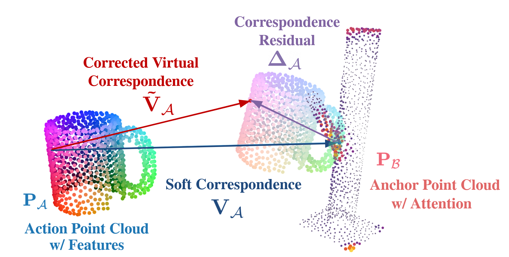
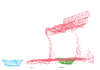
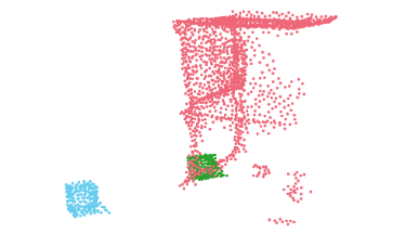
The virtual corresponding points, , given by Equation 3 in main text, are constrained to be within the convex hull of each object. However, correspondences which are constrained to the convex hull are insufficient to express a large class of desired tasks. For instance, we might want a point on the handle of a teapot to correspond to some point above a stovetop, which lies outside the convex hull of the points on the stovetop. To allow for such placements, for each point-wise embedding , we further learn a residual vector, that corrects each virtual corresponding point, allowing us to displace each virtual corresponding point to any arbitrary location that might be suitable for the task. Concretely, we use a point-wise neural network which maps each embedding into a 3D residual vector:
Applying these to the virtual points, we get a set of corrected virtual correspondences, and , defined as
| (10) |
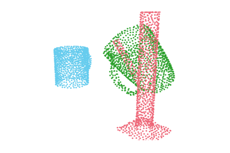
These corrected virtual correspondences define the estimated goal location relative to object for each point in object , and likewise for each point in object , as shown in Figure S.2.
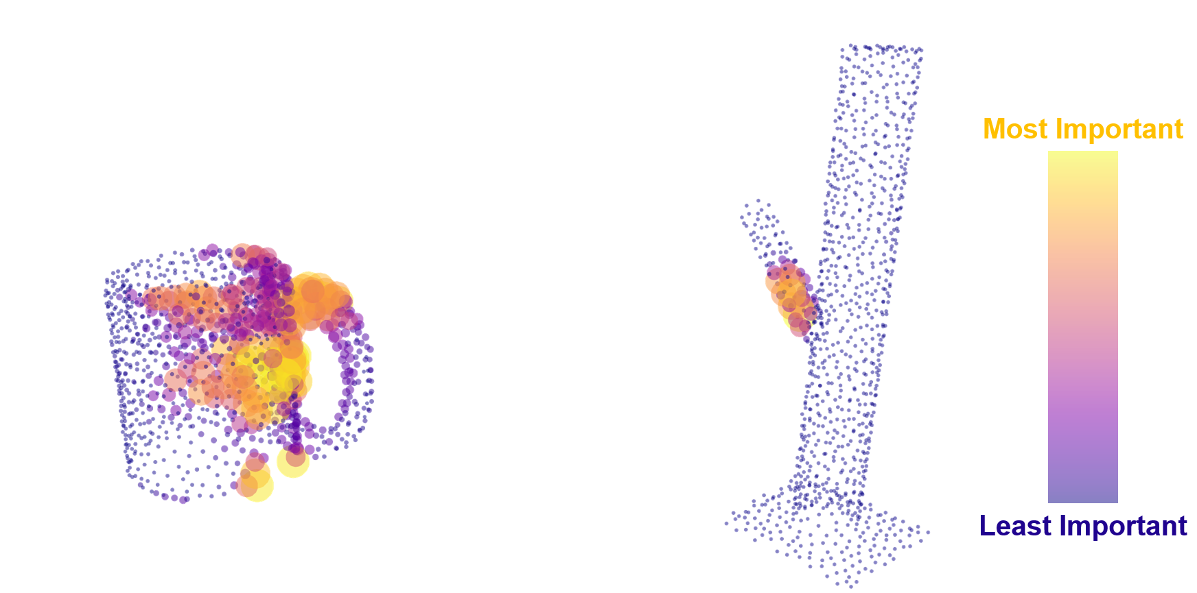
E.2 Learned Importance Weights
A visualization of the learned importance weights, and for the mug and rack are visualized by both color scheme and point size in Figure S.3
Appendix F Additional NDF Task Experiments
F.1 Further Ablations on Mug Hanging Task
In order to examine the effects of different design choices in the training pipeline, we conduct ablation experiments with final task-success (grasp, place, overall ) as evaluation metrics for Mug Hanging task with upright pose initialization for the following components of our method, see Table LABEL:tab:mug_rack_ablation_full for full ablation results. For consistency, all ablated models are trained to 15K batch steps.
-
1.
Loss. In the full pipeline reported, we use a weighted sum of the three types of losses described in Section 4.2 of the paper. Specifically, the loss used is given by
(11) where we chose , after hyperparameter search.
We ablate usage of all three types of losses, by reporting the final task performance in simulation for all experiments, specifically, we report task success on the following variants.
-
[nosep]
-
(a)
Remove the point displacement loss term, , after which we are left with
-
(b)
Remove the direct correspondence loss term, , after which we are left with
-
(c)
Remove the correspondence consistency loss term, , after which we are left with
-
(d)
From testing loss variants above, we found that the point displacement loss is a vital contributing factor for task success, where removing this loss term results in no overall task success, as shown in Table LABEL:tab:mug_rack_ablation_full. However, in practice, we have found that adding the correspondence consistency loss and direct correspondence loss generally help to lower the rotational error of predicted placement pose compared to the ground truth of collected demos. To further investigate the effects of the combination of these two loss terms, we used a scaled weighted combination of and , such that the former weight of the displacement loss term is transferred to consistency loss term, with the new , and with stays unchanged. Note that this is different from variant (a) above, as now the consistency loss given a comparable weight with dense correspondence loss term, which intuitively makes sense as the consistency loss is a function of the predicted transform to be used, while the dense correspondence loss is instead a function of the ground truth transform, , which provides a less direct supervision on the predicted transforms. Thus we are left with
-
-
2.
Usage of Correspondence Residuals. After predicting a per-point soft correspondence between objects and , we adjust the location of the predicted corresponding points by further predicting a point-wise correspondence residual vector to displace each of the predicted corresponding point. This allows the predicted corresponding point to get mapped to free space outside of the convex hulls of points in object and . This is a desirable adjustment for mug hanging task, as the desirable cross-pose usually require points on the mug handle to be placed somewhere near but not in contact with the mug rack, which can be outside of the convex hull of rack points. We ablate correspondence residuals by directly using the soft correspondence prediction to find the cross-pose transform through weighted SVD, without any correspondence adjustment via correspondence residual.
-
3.
Weighted SVD vs Non-weighted SVD. We leverage weighted SVD as described in Section 4.1 of the paper as we leverage predicted per-point weight to signify the importance of specific correspondence. We ablate the use of weighted SVD, and we use an un-weighted SVD, where instead of using the predicted weights, each correspondence is assign equal weights of , where is the number of points in the point cloud used.
-
4.
Pretraining. In our full pipeline, we pretrain the point cloud embedding network such that the embedding network is invariant. Specifically, the mug-specific embedding network is pretrained on 200 ShapeNet mug objects, while the rack-specific and gripper specific embedding network is trained on the same rack and Franka gripper used at test time, respectively. We conduct ablation experiments where
-
[nosep]
-
(a)
We omit the pretraining phase of embedding network
-
(b)
We do not finetune the embedding network during downstream training with task-specific demonstrations.
Note that in practice, we find that pretraining helps speed up the downstream training by about a factor of 3, while models with or without pretraining both reach a similar final performance in terms of task success after both models converge.
-
-
5.
Usage of Transformer as Cross-object Attention Module. In the full pipeline, we use transformer as the cross-object attention module, and we ablate this design choice by replacing the transformer architecture with a simple 3-layer MLP with ReLU activation and hidden dimension of 256, and found that this leads to worse place and grasp success.
-
6.
Dimension of Embedding. In the full pipeline, the embedding is chosen to be of dimension 512. We conduct experiment on much lower dimension of 16, and found that with dimension =16, the place success is much lower, dropped from 0.97 to 0.59.
F.2 Effects of Pretraining on Mug Hanging Task
We explore the effects of pretraining on the final task performance, as well as training convergence speed. We have found that pretraining the point cloud embedding network as described in G.1, is a helpful but not necessary component in our training pipeline. Specifically, we find that while utilizing pretraining reduces training time, allowing the model to reach similar task performance and train rotation/translation error with much fewer training steps, this component is not necessary if training time is not of concern. In fact, as see in Table LABEL:tab:no_pretraining_longer, we find that for mug hanging tasks, by training the models from scratch without our pretraining, the models are able to reach similar level of task performance of grasp, for place and for overall success rate. Furthermore, it is able to achieve similar level of train rotation error of and translation error of , compared to the models with pretraining. However, without pre-trainig, the model needs to be trained for about 5 times longer (26K steps compared to 5K steps) to reach the similar level of performance. Thus we adopt our object-level pretraining in our overall pipeline to allow lower training time.
Another benefit of pretraining is that the pretraining for each object category is done in a task-agnostic way, so the network can be more quickly adapted to new tasks after the pretraining is performed. For example, we use the same pre-trained mug embeddings for both the gripper-mug cross-pose estimation for grasping as well as the mug-rack cross-pose estimation for mug hanging.
F.3 Additional Simulation Experiments on Bowl and Bottle Placement Task
Additional results on Grasp, Place and Overall success rate in simulation for Bowl and Bottle are shown in Table LABEL:tab:bottle_bowl. For bottle and bowl experiment, we follow the same experimentation setup as in [simeonov2021neural], where the successful grasp is considered if a stable grasp of the object is obtained, and a successful place is considered when the bottle or bowl is stably placed upright on the elevated flat slab over the table without falling on the table. Reported task success results in are for both Upright Pose and Arbitrary Pose run over 100 trials each.
Appendix G Additional Training Details
G.1 Pretraining
We utilize pretraining for the embedding network for the mug hanging task, and describe the details below.
We pretrain embedding network for each object category (mug, rack, gripper), such that the embedding network is invariant with respect to the point clouds of that specific object category. Specifically, the mug-specific embedding network is pretrained on 200 ShapeNet [chang2015shapenet] mug instances, while the rack-specific and gripper-specific embedding network is trained on the same rack and Franka gripper used at test time, respectively. Note that before our pretraining, the network is randomly initialized with the Kaiming initialization scheme [he2015delving]; we don’t adopt any third-party pretrained models.
For the network to be trained to be invariant, we pre-train with InfoNCE loss [oord2018representation] with a geometric distance weighting and random transformations. Specifically, given a point cloud of an object instance, , of a specific object category , and an embedding network , we define the point-wise embedding for as , where is a -dimensional vector for each point . Given a random transformation, , we define , where is the -dimensional vector for the th point .
The weighted contrastive loss used for pretraining, , is defined as
{align}
L_wc :&= - ∑_ilog[exp(ϕi⊤ψi)∑jexp(dij(ϕi⊤ψj))]
d_ij:= {1μ tanh(λ∥p_i^A - p_j^A∥_2), \textif i ≠j
1, \textotherwise
μ:=max(tanh(λ∥p_i^A - p_j^A∥_2))
For this pretraining, we use .
Appendix H PartNet-Mobility Objects Placement Task Details
In this section, we describe the PartNet-Mobility Objects Placement experiments in detail.
H.1 Dataset Preparation
Simulation Setup. We leverage the PartNet-Mobility dataset [Xiang2020-oz] to find common household objects as the anchor object for TAX-Pose prediction. The selected subset of the dataset contains 8 categories of objects. We split the objects into 54 seen and 14 unseen instances. During training, for a specific task of each of the seen objects, we generate an action-anchor objects pair by randomly sampling transformations from as cross-poses. The action object is chosen from the Ravens simulator’s rigid body objects dataset [Zeng2020-tk]. We define a subset of four tasks (“In”, “On”, “Left” and “Right”) for each selected anchor object. Thus, there exists a ground-truth cross-pose (defined by human manually) associated with each defined specific task. We then use the ground-truth TAX-Poses to supervise each task’s TAX-Pose prediction model. For each observation action-anchor objects pair, we sample 100 times using the aforementioned procedure for the training and testing datasets.
Real-World Setup. In real-world, we select a set of anchor objects: Drawer, Fridge, and Oven and a set of action objects: Block and Bowl. We test 3 (“In”, “On”, and “Left”) TAX-Pose models in real-world without retraining or finetuning. The point here is to show the method capability of generalizing to unseen real-world objects.
H.2 Metrics
Simulation Metrics. In simulation, with access to the object’s ground-truth pose, we are able to quantitatively calculate translational and rotation error of the TAX-Pose prediction models. Thus, we report the following metrics on a held-out set of anchor objects in simulation:
| Translational Error: The L2 distance between the inferred cross-pose translation () and the ground-truth pose translation (). | Rotational Error: The geodesic distance [huynh2009metrics, hartley2013rotation] between the predicted cross-pose rotation () and the ground-truth rotation (). |
Real-World Metrics. In real-world, due to the difficulty of defining ground-truth TAX-Pose, we instead manually, qualitatively define goal “regions” for each of the anchor-action pairs. The goal-region should have the following properties:
-
[noitemsep]
-
•
The predicted TAX-Pose of the action object should appear visually correct. For example, if the specified task is “In”, then the action object should be indeed contained within the anchor object after being transformed by predicted TAX-Pose.
-
•
The predicted TAX-Pose of the action object should not violate physical constraints of the workspace and of the relation between the action and anchor objects. Specifically, the action object should not interfere with/collide with the anchor object after being transformed by the predicted TAX-Pose. See Figure S.4 for an illustration of TAX-Pose predictions that fail to meet this criterion.
H.3 Motion Planning
In both simulated and real-world experiments, we use off-the-shelf motion-planning tools to find a path between the starting pose and goal pose of the action object.
Simulation. To actuate the action object from its starting pose to its goal pose transformed by the predicted TAX-Pose , we plan a path free of collision. Learning-based methods such as [danielczuk2021object] deal with collision checking with point clouds by training a collision classifier. A more data-efficient method is by leveraging computer graphics techniques, transforming the point clouds into marching cubes [lorensen1987marching], which can then be used to efficiently reconstruct meshes. Once the triangular meshes are reconstructed, we can deploy off-the-shelf collision checking methods such as FCL [pan2012fcl] to detect collisions in the planned path. Thus, in our case, we use position control to plan a trajectory of the action object to move it from its starting pose to the predicted goal pose. We use OMPL [sucan2012open] as the motion planning tool and the constraint function passed into the motion planner is from the output of FCL after converting the point clouds to meshes via marching cubes.
![[Uncaptioned image]](https://cdn.awesomepapers.org/papers/e33f9b5e-7199-4d80-9110-186c6b580d48/realworld-setup.pdf)
Real World. In real-world experiments, we need to resolve several practical issues to make TAX-Pose prediction model viable. First, we do not have access to a mask that labels action and anchor objects. Thus, we manually define a mask by using a threshold value of -coordinate to automatically detect discontinuity in -coordinates, representing the gap of spacing between action and anchor objects upon placement. Next, grasping action objects is a non-trivial task. Since, we are only using 2 action objects (a cube and a bowl), we manually define a grasping primitive for each action object. This is done by hand-picking an offset from the centroid of the action object before grasping, and an approach direction after the robot reaches the pre-grasp pose to make contacts with the object of interest. The offsets are chosen via kinesthetic teaching on the robot when the action object is under identity rotation (canonical pose). Finally, we need to make an estimation of the action’s starting pose for motion planning. This is done by first statistically cleaning the point cloud [EisnerZhang2022FLOW] of the action object, and then calculating the centroid of the action object point cloud as the starting position. For starting rotation, we make sure the range of the rotation is not too large for the pre-defined grasping primitive to handle. Another implementation choice here is to use ICP [besl1992method] calculate a transformation between the current point cloud to a pre-scanned point cloud in canonical (identity) pose. We use the estimated starting pose to guide the pre-defined grasp primitive. Once a successful grasp is made, the robot end-effector is rigidly attached to the action object, and we can then use the same predicted TAX-Pose to calculate the end pose of the robot end effector, and thus feed the two poses into MoveIt! to get a full trajectory in joint space. Note here that the collision function in motion planning is comprised of two parts: workspace and anchor object. That is, we first reconstruct the workspace using boxes to avoid collision with the table top and camera mount, and we then reconstruct the anchor object in RViz using Octomap [hornung2013octomap] using the cleaned anchor object point cloud. In this way, the robot is able to avoid collision with the anchor object as well. See Figure S.5 for the workspace.
H.4 Goal-Conditioned Variant
We train two variants of our model, one goal-conditioned variant (TAX-Pose GC), and one task-specific variant (TAX-Pose): the only difference being that the TAX-Pose GC variant receives an encoding of the desired semantic goal position (‘top’, ‘left’, …) for the task. The goal-conditioned variant is trained across all semantic goal positions, whereas the task-specific variant is trained separately on each semantic goal category (for a total of 4 models). Importantly, both variants are trained across all PartNet-Mobility object categories. We report the performance of the variants in Table LABEL:tab:gi-Rt.
H.5 Baselines Description
In simulation, we compare our method to a variety of baseline methods.
E2E Behavioral Cloning: Generate motion-planned trajectories using OMPL that take the action object from start to goal. These serve as “expert” trajectories for Behavioral Cloning (BC). We then use a PointNet++ network to output a sparse policy that, at each time step, takes as input the point cloud observation of the action and anchor objects and outputs an incremental 6-DOF transformation that imitates the expert trajectory. The 6-DoF transformation is expressed using Euclidean translation and rotation quaternion. The “prediction” is the final achieved pose of the action object at the terminal state.
E2E DAgger: Using the same BC dataset and the same PointNet++ architecture as above, we train a sparse policy that outputs the same transformation representation as in BC using DAgger [ross2011reduction]. The “prediction” is the final achieved pose of the action object at the terminal state.
Trajectory Flow: Using the same BC dataset with DAgger, we train a dense policy using PointNet++ to predict a dense per-point 3D flow vector at each time step instead of a single incremental 6-DOF transformation. Given this dense per-point flow, we add the per-point flow to each point of the current time-step’s point cloud, and we are able to extract a rigid transformation between the current point cloud and the point cloud transformed by adding per-point flow vectors using SVD, yielding the next pose. The “prediction” is the final achieved pose of the action object at the terminal state.
Goal Flow: Instead of training a multi-step sparse/dense policy to reach the goal, train a PointNet++ network to output a single dense flow prediction which assigns a per-point 3D flow vector that points from each action object point from its starting pose directly to its corresponding goal location. Given this dense per-point flow, we add the per-point flow to each point of the start point cloud, and we are able to extract a rigid transformation between the start point cloud and the point cloud transformed by adding per-point flow vectors using SVD, yielding goal pose. We pass the start and goal pose into a motion planner (OMPL) and execute the planned trajectory. The “prediction” is thus given by the SVD output.

H.6 Per-Task Results
In the main body of the paper, we have shown the meta-results of the performance of each method by averaging the quantitative metrics for each sub-task (“In”, “On”, “Left”, and “Right” in simulation and “In”, “On” and “Left” in real-world). Here we show each sub-task’s results in Table LABEL:tab:gi-Rt_goal0111Categories from left to right: microwave, dishwasher, oven, fridge, table, washing machine, safe, and drawer., Table LABEL:tab:gi-Rt_goal1, Table LABEL:tab:gi-Rt_goal2, and Table LABEL:tab:gi-Rt_goal3 respectively.
As mentioned above, not all anchor objects have all 4 tasks due to practical reasons. For example, the doors of safes might occlude the action object completely and it is impossible to show the action object in the captured image under “Left” and “Right” tasks (due to handedness of the door); a table’s height might be too tall for the camera to see the action object under the “Top” task. Under this circumstance, for sake of simplicity and consistency, we define a subset of the 4 goals for each object such that the anchor objects of the same category have consistent tasks definitions. We show a collection of visualizations of each task defined for each category in Figure S.6.
Moreover, we also show per-task success rate for real-world experiments in Table LABEL:tab:rw_each.
Appendix I Mug Hanging Task Details
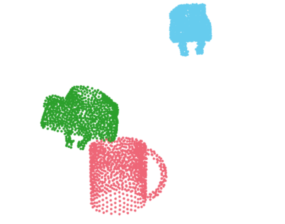
In this section, we describe the Mug Hanging task and experiments in detail. The Mug Hanging task is consisted of two sub tasks: grasp and place. A success in grasp is achieved when the mug is grasped stably by the gripper, while a success in place is achieved when the mug is hanged stably on the hanger of the rack. And the overall success mug hanging is considered when the predicted transforms enable both grasp and place success for the same trial. See Figure S.7 for a detailed breakdown of the mug hanging task in stages.

I.1 Baseline Description
In simulation, we compare our method to the results described in [simeonov2021neural].
-
[nosep]
-
•
Dense Object Nets (DON) [florence2018dense]: Using manually labeled semantic keypoints on the demonstration clouds, DON is used to compute sparse correspondences with the test objects. These correspondences are converted to a pose using SVD. A full description of usage of DON for the mug hanging task can be found in [simeonov2021neural].
-
•
Neural Descriptor Field (NDF) [simeonov2021neural]: Using the learned descriptor field for the mug, the positions of a constellation of task specific query points are optimized to best match the demonstration using gradient descent.
I.2 Training Data
To be directly comparable with the baselines we compared to, we use the exact same sets of demonstration data used to train the network in NDF [simeonov2021neural], where the data are generated via teleportation in PyBullet, collected on 10 mug instances with random pose initialization.
I.3 Training and Inference
Using the pretrained embedding network for mug and gripper, we train a grasping model for the grasping task to predict a transformation in gripper’s frame from gripper to mug to complete the grasp stage of the task. Similarly, using the pretrained embedding network for rack and mug, we train a placement model for the placing task to predict a transformation in mug’s frame from mug to rack to complete the place stage of the task. Both models are trained with the same combined loss as described in the main paper. During inference, we simply use grasping model to predict the at test time, and placement model to predict at test time.
I.4 Motion Planning
After the model predicts a transformation and , using the known gripper’s world frame pose, we calculate the desired gripper end effector pose at grasping and placement, and pass the end effector to IKFast to get the desired joint positions of Franka at grasping and placement. Next we pass the desired joint positions at gripper’s initial pose, and desired grasping joint positions to OpenRAVE motion planning library to solve for trajectory from gripper’s initial pose to grasp pose, and then grasp pose to placement pose for the gripper’s end effector.
I.5 Real-World Experiments
We pre-train the DGCNN embedding network with rotation-equivariant loss on ShapeNet mugs’ simulated point clouds in simulation. Using the pre-trained embedding, we then train the full TAX-Pose model with the 10 collected real-world point clouds.
I.6 Failure Cases
Some failure cases for TAX-Pose occur when the predicted gripper misses the rim of the mug by a xy-plane translation error, thus resulting in failure of grasp, as seen in Figure 8(a). A common failure mode for the mug placement subtask is characterized by an erroneous transform prediction that results in the mug’s handle completely missing the rack hanger, thus resulting in placement failure, as seen in Figure 8(b).