TarGF: Learning Target Gradient Field to Rearrange Objects without Explicit Goal Specification
Abstract
Object Rearrangement is to move objects from an initial state to a goal state. Here, we focus on a more practical setting in object rearrangement, i.e., rearranging objects from shuffled layouts to a normative target distribution without explicit goal specification. However, it remains challenging for AI agents, as it is hard to describe the target distribution (goal specification) for reward engineering or collect expert trajectories as demonstrations. Hence, it is infeasible to directly employ reinforcement learning or imitation learning algorithms to address the task. This paper aims to search for a policy only with a set of examples from a target distribution instead of a handcrafted reward function. We employ the score-matching objective to train a Target Gradient Field (TarGF), indicating a direction on each object to increase the likelihood of the target distribution. For object rearrangement, the TarGF can be used in two ways: 1) For model-based planning, we can cast the target gradient into a reference control and output actions with a distributed path planner; 2) For model-free reinforcement learning, the TarGF is not only used for estimating the likelihood-change as a reward but also provides suggested actions in residual policy learning. Experimental results in ball rearrangement and room rearrangement demonstrate that our method significantly outperforms the state-of-the-art methods in the quality of the terminal state, the efficiency of the control process, and scalability. The code and demo videos are on https://sites.google.com/view/targf. {NoHyper} ††* indicates equal contribution
1 Introduction

As shown in Fig. 1, we consider object rearrangement without explicit goal specification ICML12Arrange ; abdo2015robot , where the agent is required to manipulate a set of objects from an initial layout to a normative distribution. This task is taken for granted by humans ricciuti1965object and widely exists in our daily life, such as tidying up a table neatnet , placing furniture wang2020scene , and sorting parcels kim2020sortation .
However, compared with conventional robot tasks yu2020meta ; zhu2017target ; luo2019end ; kiran2021deep ; zuo2019craves , there are two critical challenges in our setting: 1) Hard to clearly define the target state (goal), as the target distribution is diverse and the patterns are difficult to describe in the program, e.g., how to evaluate the tidiness quantitatively? As a result, it is difficult to manually design a reward/objective function, which is essential to modern control methods, e.g., deep reinforcement learning (DRL) mnih2015human . 2) In the physical world, the agents also need to find an executable path to reach the target state efficiently and safely, i.e., finding a short yet collision-free path to reach the target distribution. To this end, the agents are required to jointly learn to evaluate the quality of the state (reward) and move objects to increase the quality efficiently. In other words, the agents should answer the two questions: What kind of layouts does the user prefer, and How to manipulate objects to meet the target distribution?
Thus, searching for a policy without dependence on the explicit goal state and shaped reward is necessary. Imitation learning (IL) can learn a reward function ho2016generative ; SQIL2019 ; EBIL or learn a policy BC1 ; BC2 ; BC3 ; zhong2021towards from the expert’s supervision, e.g., demonstrating expected trajectories. However, collecting a large number of expert trajectories is expensive. Recently, example-based reinforcement learning (RL) VICE2018 ; RCE has tried to reduce the reliance on expert trajectories, i.e., learning a policy only with examples of successful outcomes. However, it is still difficult to learn a classifier to provide accurate reward signals for learning in the case of high-dimensional state and action space, as there are many objects to control in object rearrangements.
In this work, we separate the task into two stages: 1) learning a score function to estimate the target-likelihood-change between adjacent states, and 2) learning/building a policy to rearrange objects with the score function. Inspired by the recent advances in score-based generative models VanillaScoreMatching ; SDEScoreMatching ; 21Molecule ; LST ; SDEdit , we employ the denoising score-matching objective denosingScoreMatching to train a target score network for estimating the target gradient field, i.e., the gradient of the log density of the target distribution. The target gradient field can be viewed as object-wise guidance that provides a pseudo velocity for each object, pointing to regions with a higher density of the target distribution, e.g., tidier configurations. To rearrange objects in the physical world, we demonstrate two ways to leverage the target gradient field in control. 1) We integrate the gradient-based guidance with a model-based path planner to rearrange objects without collision. 2) We further derive a reward function for reinforcement learning by estimating the likelihood change via the target gradient. With the TarGF-based reward and a TarGF-guided residual policy network Residual , we can train an effective RL-based policy.
In experiments, we evaluate the effectiveness of our methods on two typical rearrangement tasks: Ball Rearrangement and Room Rearrangement. First, we introduce three metrics to analyse the quality of the terminal state and the efficiency of the control process. In Ball Rearrangement, we demonstrate that our control methods can efficiently reach a high-quality and diverse terminal configuration. We also observe that our methods can find a path with fewer collisions and shorter lengths to converge compared with learning-based baselines SQIL2019 ; RCE and planning-based baselines ORCA . In Room Rearrangement, we further evaluate our methods’ feasibility in complex scenes with multiple heterogeneous objects.
Our contributions are summarised as follows:
-
•
We introduce a novel score-based framework that estimates a target gradient field (TarGF) via denoising score matching for object rearrangement.
-
•
We point out two usages of the target gradient field in object rearrangement: 1) providing guidance in moving direction; 2) deriving a reward for learning.
-
•
We conduct experiments to demonstrate that both traditional planning and RL methods can benefit from the target gradient field and significantly outperform the state-of-the-art methods in sample diversity, realism and safety.
2 Related Works
2.1 Object and Scene (Re-)Arrangement
The object (re-)arrangement is a long-studied problem in robotics community abdo2015robot ; schuster2012learning ; abdo2016organizing and the graphics community fisher2012example ; MakeItHome2011 ; RJMCMC2012 ; SceneNet2016 ; songchun2018 . However, most of them focus on manually designing rules/ energy functions to find a goal abdo2015robot ; schuster2012learning ; abdo2016organizing or synthesising a scene configuration MakeItHome2011 ; RJMCMC2012 ; SceneNet2016 ; songchun2018 that satisfies the preference of the user. The most recent work neatnet tries to learn a GNN to output an arrangement tailored to human preferences. However, they neglect the physical process of rearrangement. Hence, the accessibility and transition costs from the initial and target states are not guaranteed. Considering the physical interaction, the recent works on scene rearrangement rearrange ; visualrearrange mitigate the goal specification problem by providing a goal scene to the agent, making the reward shaping feasible. Concurrent works ECCV22HouseKeep ; ECCV22TIDEE also notice the necessity of automatic goal inference for tying rooms and exploit the commonsense knowledge from Large Language Model (LLM) or memex graph to infer rearrangements goals when the goal is unspecified. Another concurrent work ICML22Arrangement aims at discovering generalisable spatial goal representations via graph-based active reward learning for 2D object rearrangement. In this paper, we focus on a more practical setting of rearrangement: how to estimate the similarity (i.e., the target likelihood) between the current state and the example sets and manipulate objects to maximise it. Here, only a set of positive target examples are required to learn the gradient field rather than prior knowledge about specific scenarios.
2.2 Learning without Reward Engineering
Without hand-engineered reward, previous works explore algorithms to learn a control policy from expert demonstrations via behavioural cloning BC1 ; BC2 ; BC3 ; ho2016generative or inverse reinforcement learning AIRL ; EBIL ; DAC ; MaxEntIRL . Imitation learning (IL) BC1 ; BC2 ; BC3 aims to directly learn a policy by cloning the behaviour from the expert trajectories. The inverse reinforcement learning (IRL) AIRL ; EBIL ; DAC ; MaxEntIRL tries to learn a reward function from data for subsequent reinforcement learning. Considering the difficulty in collecting expert trajectories, some example-based methods are proposed to learn a policy only with a set of successful examples VICE2018 ; SQIL2019 ; RCE . The most recent work is RCE RCE which directly learns a recursive classifier from successful outcomes and interactions for policy optimisation. We also try to develop an example-based control method for rearrangement with a set of examples. Our method can learn the target gradient field from the examples without any additional effort in reward engineering. The target gradient field can provide meaningful reward signals and action guidance for reinforcement learning and traditional path planners. To the best of our knowledge, such usage of gradient field is not explored in previous works.
3 Problem Statement
We aim to learn a policy that moves objects to reach states close to a target distribution without relying on reward engineering. Similar to the example-based control RCE , the grounded target distribution is unknown to the agent, and the agent is only given a set of target examples where . In practice, these examples can be provided by the user without accessing the dynamics of the robot. The agent starts from an initial state , where objects are randomly placed in the environment. At time step , the agent takes action imposed on the objects to reach the next state with dynamics . Here, the goal of the agent is to search for a policy that maximises the discounted log-target-likelihood of the future states:
| (1) |
where denotes the discount factor. Notably, we assume that everywhere since we can perturb the original data with a tiny noise (e.g., ) to ensure the perturbed density is always positive. VanillaScoreMatching also used this trick to tackle the manifold hypothesis issue. This objective reveals three challenges: 1) Inaccessibility problem: The grounded target distribution in Eq. 1 is inaccessible. Thus, we need to learn a function to approximate the log-target-likelihood for policy search. 2) Sparsity problem: The log-target-likelihood is sparse in the state space due to the Manifold Hypothesis mentioned in VanillaScoreMatching . Hence, even if we have access to the target distribution , it is still difficult to explore the high-density region. 3) Adaptation problem: The dynamics is also inaccessible. To maximise the cumulative sum in Eq. 1, the agent is required to adapt to the dynamics to efficiently increase the target likelihood.
To address these problems, we partition the task into 1) learning to estimate the log-target-likelihood (reward) of the state and 2) learning/building a policy to rearrange objects to adapt to the dynamics.
4 Method

4.1 Motivation
Estimating the gradient of the log-target-likelihood can tackle the first two problems mentioned in Sec. 3: For the inaccessibility problem, we can approximate the likelihood increment between two adjacent states by the first-order Taylor expansion . This helps to derive a surrogate objective (i.e., Eq. 4) of Eq. 1.
For the sparsity problem, we can leverage the gradient field to help with exploration since the gradient indicates the fastest direction to increase the target likelihood. To estimate , we employ the score-matching SDEScoreMatching , a novel generative model that achieved impressive results in many research areas recently21Molecule ; SDEdit ; LST , to train a target score network .
To address the adaptation problem, we further demonstrate two approaches to incorporate the trained target gradient field with control algorithms for object rearrangement: 1) For the model-based setting, our framework casts the target gradient into a reference control and outputs an action with a distributed path planner. 2) For the model-free setting (reinforcement learning), we leverage the target gradient to estimate reward and provide suggested action in residual policy learning Residual .
4.2 Learning the Target Gradient Field from Examples
The target score network is the core module of our framework, which aims at estimating the score function (i.e.the gradient of log-density) of the target distribution .
To train the target score network, we adopt the Denoising Score-Matching (DSM) objective proposed by denosingScoreMatching , which can guarantee a reasonable estimation of the . In training, we pre-specify a noise distribution . Then, DSM matches the output of the target score network with the score of the perturbed target distribution :
| (2) |
The DSM objective guarantees the optimal score network satisfies almost surely. When is small enough, we have , so that .
In practice, we adopt a variant of DSM proposed by SDEScoreMatching , which conducts DSM under different noise scales simultaneously. This way, we can efficiently try different noise scales after only one training. The target score network is implemented as a graph-based network , which is conditioned on a noise level . The input state is constructed as a fully-connected graph that takes each object’s state (e.g.position, orientation) and static properties (e.g.category, bounding-box) as the node feature . The input graph is pre-processed by linear feature extraction layers and then passed through several Edge-Convolution layers. After message-passing, the output on the i-th node serves as the component of the target gradient on the i-th object’s state . We defer structure details to Appendix. B.
4.3 Model-based Planning with the Target Gradient Field
The target gradient can be translated into a gradient-based action , where denotes the gradient-to-action translation. A gradient over the state space can be viewed as velocities imposed on each object. For instance, if the state of each object is a 2-dimensional position , then the target gradient component on the i-th object can be viewed as linear velocities on two axes . When the action space is also velocities, we can construct by simply projecting the target gradient into the action space , where the denotes the speed limit. Following the gradient-based action, objects will move towards directions that may increase the likelihood of the next state, which meets the need for the rearrangement task.
However, the gradient-based action will potentially lead objects to collide with each other since the target gradient cannot infer the environment constraints from only target examples.
To adapt the gradient-based action to the environment dynamics, we incorporate the target gradient field with a model-based off-the-shelf collision-avoidance algorithm ORCA. The ORCA planner takes the gradient-based action as reference velocities and then outputs the collision-free velocities with the least modification to the reference velocities. In this way, the adapted action can lead objects to move towards a higher likelihood region efficiently and safely. For more details of the ORCA planner, we defer to Appendix B.2.
4.4 Learning Policy with the Target Gradient Field
The model-based approach to ‘correct’ the target gradient assumes the objects are of circular shape. This limits the scope of this method when objects are of non-circular shape (e.g., furniture). To this end, we propose a model-free approach based on reinforcement learning (RL) for object rearrangement, where the agent needs to adapt the dynamics via online interactions.
To tackle the inaccessibility problem mentioned in Sec. 3, we first derive an equivalent of the original objective in Eq. 1 by subtracting a constant from the original objective:
| (3) | ||||
Further, we derive a surrogate objective to approximate the . We notice that in most physical simulated tasks, the distance between two adjacent states is quite small, which inspires us to approximate the log-likelihood-change of the adjacent states using the Taylor expansion:
| (4) |
In this way, we can optimise the surrogate objective by assigning as the immediate reward. In practice, we simply assign the last term of the cumulative summation as the immediate reward , and this version is shown to be the most effective.
To further tackle the sparsity problem, our idea is to build a residual policy upon the gradient-based action mentioned in Sec. 4.3, as helps to explore the regions with a high target likelihood:
| (5) |
This approach is similar to the residual policy learning proposed by Residual . The serves as an initial policy, and the residual policy network takes the target gradient and the current state as input and outputs to ‘correct’ the . The agent finally outputs a ‘corrected’ action . In this way, the agent can benefit from the efficient exploration and have less training burden as it ‘stands on the giant’s shoulder’ (i.e.the gradient-based action ).
We employ the multi-agent Soft-Actor-Critic(SAC) SAC as the reinforcement learning algorithm backbone. Each object is regarded as an agent and can communicate with all the other agents. At each time step , the reward for the i-th agent is , where is a centralised target likelihood reward, is a hyperparameter and is a decentralised collision penalty where is a collision penalty. Specifically, when a collision is detected between object and , , otherwise .
5 Experiment Setups
5.1 Environment
We design two object rearrangement tasks without explicit goal specification for evaluation: Ball Rearrangement and Room Rearrangement, where the former uses controlled environments for better numerical analysis and the latter is built on a real dataset with implicit target distribution.
Ball Rearrangement includes three environments with increasing difficulty: Circling, Clustering, and the hybrid of the first two, Circling + Clustering, as shown in Fig. 3. There are 21 balls of the same geometry in each task. The balls are divided equally into three colours in Clustering and Circling+Clustering. The goals of the three tasks are as follows: Circling requires all balls to form a circle. The circle’s centre can be anywhere in the environment; Clustering requires all balls to form into three clusters by colour. The joint centre of each cluster has two choices (i.e., red-green-blue or red-blue-green clockwise); Circling + Clustering requires all balls to form into a circle where balls of the same type are adjacent. To slightly increase the complexity of the physical dynamics, we enlarge the lateral friction coefficient of each ball and make each ball with different physical properties, e.g., different friction coefficients and masses. The target examples of each task are sampled from an explicit process. Thus, we can define a ‘pseudo likelihood’ on a given state according to the sampling process to measure the similarity between the state and the target distribution.

Room Rearrangement is built on a more realistic dataset, 3D-FRONT 3dfront . After cleaning the data, we get a dataset with 839 rooms, 756 for training, e.g., target examples, and 83 for testing. In each episode, we sample a room from the test split and shuffle the room via a Brownian Process at the beginning to get an initial state. The agent can assign angular and linear velocities for each object in the room at each time step. To tidy up the room, the agent must learn implicit knowledge from the target examples, as shown in Fig. 4. More details are in the Appendix A.

5.2 Evaluation
For baseline comparison and ablation studies, we collect a fixed number of trajectories starting from the same initial states for each of the 5 random seeds. For each random seed, we collect 100 and (8 initial states for each room) trajectories for ball and room rearrangement, respectively. Then we calculate the following metrics on the trajectories, where the PL is only reported in ball rearrangement. More details of evaluation are in the Appendix D.
Pseudo-Likelihood (PL) measures the efficiency of the rearrangement process and the sample quality of the results. We specify a pseudo-likelihood function for each environment that measures the similarity between a given state and the target examples. For each time step , we report the mean PL over trajectories and the confidence interval over 5 random seeds. We do not report PL on room rearrangement as it is hard to program human preferences.
Coverage Score (CS) measures the diversity and fidelity of the rearrangement results (i.e.the terminal states of the trajectories) by calculating the Minimal-Matching-Distance (MMD) MMD between and a fixed set of examples from : . If the rearrangement results of a method miss some modes in the ground truth example set, the coverage score will increase to hurt the performance.
Averaged Collision Number (ACN) reflects the safety and efficiency of the rearrangement process since object collision will lead to object blocking and deceleration. ACN is calculated as , where denotes the total collision number at time step .
5.3 Baselines
We compare our framework, i.e., Ours (ORCA) and Ours (SAC), with planning-based baselines and learning-based baselines. Besides, we design heuristic baselines as the upper bounds for ball rearrangement tasks. All the reinforcement learning-based methods share the same network design, capacity and hyperparameters. More details of baselines are in Appendix. C.
Leaning-based Baselines: GAIL: A classical inverse RL method that trains a discriminator as the reward function. RCE: A strong example-based reinforcement learning method proposed recently. SQIL: A competitive example-based imitation learning method. Goal-RL: An ‘open-loop’ method that first generates a goal at the beginning of the episode via a VAE trained from the target examples and then trains a goal-conditioned policy to reach the proposed goal via RL.
Planning-based Baselines: Goal (ORCA): This method first generates a goal via the same VAE as in Goal (SAC). Then the agent assigns an action pointing to the goal as reference control and adjusts the preference velocity using ORCA, similar to Sec. 4.3.
Heuristic-based Baseline: Oracle: We slightly perturb the samples from the target distribution and take these samples as the rearrangement results. This method’s rearrangement results will be close to the target distribution yet different from the target examples. Hence, we use this method to normalise the PL curve and CS bars.


6 Result Analysis
6.1 Baseline Comparison
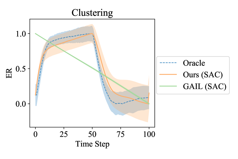
Ball Rearrangement: We present the quantitative results on ball rearrangement tasks in the first three columns of Fig. 5. As shown on the top row of Fig. 5, the PL curves of Ours (SAC) and Ours (ORCA) are significantly higher and steeper than all the baselines in all three tasks, which shows the effectiveness of our method in arranging objects towards the target distribution efficiently. In the middle row of Fig. 5, Ours (ORCA) achieves the best performance in CS across all three tasks. Goal (SAC) outperforms Ours (SAC) on Clustering and Circling+Clustering since the goal is proposed by a generative model that can naturally generate diverse and realistic goals. From the qualitative results shown in Fig. 3, our methods, especially Ours (ORCA), also outperform the baselines in realism. Our methods also achieve the lowest ACN in most cases, except that Goal (SAC) is slightly better than Ours (SAC) in Circling.
The Goal (SAC) is the strongest baseline yet loses to our framework in efficiency since the generated goals are far from the initial state. We validate this problem by comparing the averaged path length of the Goal (SAC) with ours in Appendix. E.3. Results show that our methods converge in a shorter path than goal-based baselines across all three tasks. Besides, the Goal (SAC) suffers from invalid goal proposals. As shown in Fig. 3, the Goal (SAC) and Goal (ORCA) can rearrange objects in the right trend, but the objects may block each other’s way. This is because the goals generated by the VAE are not guaranteed to be valid (e.g.the balls may overlap with each other), so the agent cannot reach the invalid goal. We demonstrate this problem in Appendix. E.4.
The classifier-based reward learning method, GAIL, RCE, and SQIL, basically fails in most tasks, as shown in Fig. 3 and Fig. 5. This is due to the over-exploitation problem that commonly exists in classifier-based reward learning methods. We validate this in Appendix E.2.
Room Rearrangement: We only compare Ours (SAC) with learning-based baselines because it is infeasible to employ the ORCA planner in room rearrangement since all the furniture is non-circular. As shown in Fig. 4, our method can obtain more realistic rearrangement results than baselines. As shown in the last column of Fig. 5, the coverage score of Ours (SAC) is the lowest and almost half of that of Goal (SAC). Meanwhile, Ours (SAC) achieves the lowest ACN compared with baselines. These results prove our method can work on a more complex task and generalise well to unseen conditions.
6.2 Ablation Studies and Analysis
We conduct ablation studies on ball rearrangement tasks to investigate: 1) The effectiveness of the exploration guidance provided from the target gradient field and 2) The necessity of combining the target gradient field with control algorithms to adapt to the environment dynamics. To this end, we construct an ablated version named Ours w/o Residual that drops the residual policy learning and another named Ours w/o RL that only takes gradient-based action as policy.

Ours w/o Residual: The CS bars in Fig. 5 shows that Ours (SAC) significantly outperforms the Ours w/o Residual in CS, which means the agent is easy to over-exploit few modes with high density. We also show qualitative results in Appendix E.1 that the objects are usually arranged into a single pattern without the residual policy learning.
Ours w/o RL: The PL curves in Fig. 5 show that without the control algorithm serving as the backbone, the rearrangement efficiency of Ours w/o RL is significantly lower than Ours (SAC) and Ours (ORCA). Meanwhile, the ACN of Ours w/o RL is significantly larger than Ours (SAC) and Ours (ORCA), which indicates the gradient-based action may cause severe collisions without adapting to the environment dynamics.
Scalability: We further evaluate the scalability of our methods by zero-shot transferring the learned model to rearrange different numbers of objects. Specifically, we train all the policies in the ball environment with balls. During the testing phase, we directly transfer each policy to environments with increased ball numbers, i.e., , , and , without any fine-tuning. In Fig. 6, we report the averaged PL increment from each method’s initial to target states. Results show that our method still outperforms baselines under different numbers of balls.
7 Conclusion
In this study, we first analyse the challenges of object rearrangement without explicit goal specification and then incorporate a target gradient field with either model-based planning or model-free learning approaches to achieve this task. Experiments demonstrate our effectiveness by comparisons with learning-based and planning-based baselines.
Limitation and Future Works. This work only considers the planar state-based rearrangement with simplified environments where the agent can directly control the velocities of objects. In future works, it is necessary to extend our framework to more realistic scenarios, e.g., manipulating objects by robots in a realistic 3D environment zuo2019craves ; qiu2017unrealcv . We summarise the future directions in the following:
-
•
Visual Observation: We may explore how to conduct efficient and accurate score-based reward estimation from image-based examples and leverage the recent progress on visual state representation learning worldmodel1 ; worldmodel2 ; worldmodel3 ; zhong2019ad to develop the visual gradient-based action.
-
•
Complex Dynamics: When the agent can only move one object at a time, we may explore hierarchical methods where high-level policy chooses which object to move and low-level policy leverages the gradient-based action for motion planning. When we can only impose forces on objects instead of velocities, we may explore a hierarchical policy where a high-level policy outputs target velocities and a low-level employ a velocity controller, such as a PID controller, to mitigate the velocity errors.
-
•
Multi-Agent Scenarios: The framework can also be extended to multi-agent scenarios zhong2021towards ; wang2022tomc ; xu2020learning ; pan2022mate , where the decentralised agents need to estimate its gradient field and take actions according to the local observation for multi-agent cooperation or competition.
Ethics Statement. Our method has the potential to build home-assistant robots. We evaluate our method in simulated environments, which may introduce data bias. However, similar studies also have such general concerns. We do not see any possible major harm in our study.
Acknowledgement
This work was supported by the National Natural Science Foundation of China -Youth Science Fund (No.62006006): Learning Visual Prediction of Interactive Physical Scenes using Unlabelled Videos and China National Post- doctoral Program for Innovative Talents (Grant No. BX2021008). We also thank Yizhou Wang, Tianhao Wu and Yali Du for their insightful discussions.
References
- (1) Yun Jiang, Marcus Lim, and Ashutosh Saxena. Learning object arrangements in 3d scenes using human context. In ICML, 2012.
- (2) Nichola Abdo, Cyrill Stachniss, Luciano Spinello, and Wolfram Burgard. Robot, organize my shelves! tidying up objects by predicting user preferences. In 2015 IEEE International Conference on Robotics and Automation (ICRA), pages 1557–1564. IEEE, 2015.
- (3) Henry N Ricciuti. Object grouping and selective ordering behavior in infants 12 to 24 months old. Merrill-Palmer Quarterly of Behavior and Development, 11(2):129–148, 1965.
- (4) Ivan Kapelyukh and Edward Johns. My house, my rules: Learning tidying preferences with graph neural networks. In 5th Annual Conference on Robot Learning, 2021.
- (5) Hanqing Wang, Wei Liang, and Lap-Fai Yu. Scene mover: Automatic move planning for scene arrangement by deep reinforcement learning. ACM Transactions on Graphics (TOG), 39(6):1–15, 2020.
- (6) Ju-Bong Kim, Ho-Bin Choi, Gyu-Young Hwang, Kwihoon Kim, Yong-Geun Hong, and Youn-Hee Han. Sortation control using multi-agent deep reinforcement learning in n-grid sortation system. Sensors, 20(12):3401, 2020.
- (7) Tianhe Yu, Deirdre Quillen, Zhanpeng He, Ryan Julian, Karol Hausman, Chelsea Finn, and Sergey Levine. Meta-world: A benchmark and evaluation for multi-task and meta reinforcement learning. In Conference on Robot Learning, pages 1094–1100. PMLR, 2020.
- (8) Yuke Zhu, Roozbeh Mottaghi, Eric Kolve, Joseph J Lim, Abhinav Gupta, Li Fei-Fei, and Ali Farhadi. Target-driven visual navigation in indoor scenes using deep reinforcement learning. In 2017 IEEE International Conference on Robotics and Automation (ICRA), pages 3357–3364. IEEE, 2017.
- (9) Wenhan Luo, Peng Sun, Fangwei Zhong, Wei Liu, Tong Zhang, and Yizhou Wang. End-to-end active object tracking and its real-world deployment via reinforcement learning. IEEE Transactions on Pattern Analysis and Machine Intelligence, 42(6):1317–1332, 2019.
- (10) B Ravi Kiran, Ibrahim Sobh, Victor Talpaert, Patrick Mannion, Ahmad A Al Sallab, Senthil Yogamani, and Patrick Pérez. Deep reinforcement learning for autonomous driving: A survey. IEEE Transactions on Intelligent Transportation Systems, 2021.
- (11) Yiming Zuo, Weichao Qiu, Lingxi Xie, Fangwei Zhong, Yizhou Wang, and Alan L Yuille. Craves: Controlling robotic arm with a vision-based economic system. In Proceedings of the IEEE/CVF Conference on Computer Vision and Pattern Recognition, pages 4214–4223, 2019.
- (12) Volodymyr Mnih, Koray Kavukcuoglu, David Silver, Andrei A Rusu, Joel Veness, Marc G Bellemare, Alex Graves, Martin Riedmiller, Andreas K Fidjeland, Georg Ostrovski, et al. Human-level control through deep reinforcement learning. Nature, 518(7540):529–533, 2015.
- (13) Jonathan Ho and Stefano Ermon. Generative adversarial imitation learning. Advances in Neural Information Processing Systems, 29:4565–4573, 2016.
- (14) Siddharth Reddy, Anca D. Dragan, and Sergey Levine. {SQIL}: Imitation learning via reinforcement learning with sparse rewards. In International Conference on Learning Representations, 2020.
- (15) Minghuan Liu, Tairan He, Minkai Xu, and Weinan Zhang. Energy-based imitation learning. arXiv preprint arXiv:2004.09395, 2020.
- (16) Dean A Pomerleau. Efficient training of artificial neural networks for autonomous navigation. Neural Computation, 3(1):88–97, 1991.
- (17) Stéphane Ross and Drew Bagnell. Efficient reductions for imitation learning. In Proceedings of the thirteenth international conference on artificial intelligence and statistics, pages 661–668. JMLR Workshop and Conference Proceedings, 2010.
- (18) Stéphane Ross, Geoffrey J. Gordon, and J. Andrew Bagnell. A reduction of imitation learning and structured prediction to no-regret online learning. In AISTATS, 2011.
- (19) Fangwei Zhong, Peng Sun, Wenhan Luo, Tingyun Yan, and Yizhou Wang. Towards distraction-robust active visual tracking. In International Conference on Machine Learning, pages 12782–12792. PMLR, 2021.
- (20) Justin Fu, Avi Singh, Dibya Ghosh, Larry Yang, and Sergey Levine. Variational inverse control with events: A general framework for data-driven reward definition. Advances in Neural Information Processing Systems, 31, 2018.
- (21) Ben Eysenbach, Sergey Levine, and Russ R Salakhutdinov. Replacing rewards with examples: Example-based policy search via recursive classification. Advances in Neural Information Processing Systems, 34:11541–11552, 2021.
- (22) Yang Song and Stefano Ermon. Generative modeling by estimating gradients of the data distribution. Advances in Neural Information Processing Systems, 32, 2019.
- (23) Yang Song, Jascha Sohl-Dickstein, Diederik P Kingma, Abhishek Kumar, Stefano Ermon, and Ben Poole. Score-based generative modeling through stochastic differential equations. In International Conference on Learning Representations, 2021.
- (24) Chence Shi, Shitong Luo, Minkai Xu, and Jian Tang. Learning gradient fields for molecular conformation generation. In International Conference on Machine Learning, pages 9558–9568. PMLR, 2021.
- (25) Shitong Luo and Wei Hu. Score-based point cloud denoising. In Proceedings of the IEEE/CVF International Conference on Computer Vision, pages 4583–4592, 2021.
- (26) Chenlin Meng, Yutong He, Yang Song, Jiaming Song, Jiajun Wu, Jun-Yan Zhu, and Stefano Ermon. Sdedit: Guided image synthesis and editing with stochastic differential equations. In International Conference on Learning Representations, 2021.
- (27) Pascal Vincent. A connection between score matching and denoising autoencoders. Neural Computation, 23(7):1661–1674, 2011.
- (28) Tom Silver, Kelsey Allen, Josh Tenenbaum, and Leslie Kaelbling. Residual policy learning. arXiv preprint arXiv:1812.06298, 2018.
- (29) Jur van den Berg, Stephen J Guy, Ming Lin, and Dinesh Manocha. Reciprocal n-body collision avoidance. In Robotics Research, pages 3–19. Springer, 2011.
- (30) Martin J Schuster, Dominik Jain, Moritz Tenorth, and Michael Beetz. Learning organizational principles in human environments. In 2012 IEEE International Conference on Robotics and Automation, pages 3867–3874. IEEE, 2012.
- (31) Nichola Abdo, Cyrill Stachniss, Luciano Spinello, and Wolfram Burgard. Organizing objects by predicting user preferences through collaborative filtering. The International Journal of Robotics Research, 35(13):1587–1608, 2016.
- (32) Matthew Fisher, Daniel Ritchie, Manolis Savva, Thomas Funkhouser, and Pat Hanrahan. Example-based synthesis of 3d object arrangements. ACM Transactions on Graphics (TOG), 31(6):1–11, 2012.
- (33) Lap Fai Yu, Sai Kit Yeung, Chi Keung Tang, Demetri Terzopoulos, Tony F Chan, and Stanley J Osher. Make it home: automatic optimization of furniture arrangement. ACM Transactions on Graphics (TOG)-Proceedings of ACM SIGGRAPH 2011, v. 30,(4), July 2011, article no. 86, 30(4), 2011.
- (34) Yi-Ting Yeh, Lingfeng Yang, Matthew Watson, Noah D Goodman, and Pat Hanrahan. Synthesizing open worlds with constraints using locally annealed reversible jump mcmc. ACM Transactions on Graphics (TOG), 31(4):1–11, 2012.
- (35) Ankur Handa, Viorica Pătrăucean, Simon Stent, and Roberto Cipolla. Scenenet: An annotated model generator for indoor scene understanding. In 2016 IEEE International Conference on Robotics and Automation (ICRA), pages 5737–5743. IEEE, 2016.
- (36) Siyuan Qi, Yixin Zhu, Siyuan Huang, Chenfanfu Jiang, and Song-Chun Zhu. Human-centric indoor scene synthesis using stochastic grammar. In Proceedings of the IEEE Conference on Computer Vision and Pattern Recognition, pages 5899–5908, 2018.
- (37) Dhruv Batra, Angel X Chang, Sonia Chernova, Andrew J Davison, Jia Deng, Vladlen Koltun, Sergey Levine, Jitendra Malik, Igor Mordatch, Roozbeh Mottaghi, et al. Rearrangement: A challenge for embodied ai. arXiv preprint arXiv:2011.01975, 2020.
- (38) Luca Weihs, Matt Deitke, Aniruddha Kembhavi, and Roozbeh Mottaghi. Visual room rearrangement. In Proceedings of the IEEE/CVF Conference on Computer Vision and Pattern Recognition, pages 5922–5931, 2021.
- (39) Yash Kant, Arun Ramachandran, Sriram Yenamandra, Igor Gilitschenski, Dhruv Batra, Andrew Szot, and Harsh Agrawal. Housekeep: Tidying virtual households using commonsense reasoning. arXiv preprint arXiv:2205.10712, 2022.
- (40) Gabriel Sarch, Zhaoyuan Fang, Adam W Harley, Paul Schydlo, Michael J Tarr, Saurabh Gupta, and Katerina Fragkiadaki. Tidee: Tidying up novel rooms using visuo-semantic commonsense priors. arXiv preprint arXiv:2207.10761, 2022.
- (41) Aviv Netanyahu, Tianmin Shu, Joshua Tenenbaum, and Pulkit Agrawal. Discovering generalizable spatial goal representations via graph-based active reward learning. In International Conference on Machine Learning, pages 16480–16495. PMLR, 2022.
- (42) Justin Fu, Katie Luo, and Sergey Levine. Learning robust rewards with adverserial inverse reinforcement learning. In International Conference on Learning Representations, 2018.
- (43) Ilya Kostrikov, Kumar Krishna Agrawal, Debidatta Dwibedi, Sergey Levine, and Jonathan Tompson. Discriminator-actor-critic: Addressing sample inefficiency and reward bias in adversarial imitation learning. In International Conference on Learning Representations, 2019.
- (44) Brian D Ziebart, Andrew L Maas, J Andrew Bagnell, Anind K Dey, et al. Maximum entropy inverse reinforcement learning. In Aaai, volume 8, pages 1433–1438. Chicago, IL, USA, 2008.
- (45) Tuomas Haarnoja, Aurick Zhou, Pieter Abbeel, and Sergey Levine. Soft actor-critic: Off-policy maximum entropy deep reinforcement learning with a stochastic actor. In Jennifer Dy and Andreas Krause, editors, Proceedings of the 35th International Conference on Machine Learning, volume 80 of Proceedings of Machine Learning Research, pages 1861–1870. PMLR, 10–15 Jul 2018.
- (46) Huan Fu, Bowen Cai, Lin Gao, Ling-Xiao Zhang, Jiaming Wang, Cao Li, Qixun Zeng, Chengyue Sun, Rongfei Jia, Binqiang Zhao, et al. 3d-front: 3d furnished rooms with layouts and semantics. In Proceedings of the IEEE/CVF International Conference on Computer Vision, pages 10933–10942, 2021.
- (47) Panos Achlioptas, Olga Diamanti, Ioannis Mitliagkas, and Leonidas Guibas. Learning representations and generative models for 3d point clouds. In International Conference on Machine Learning, pages 40–49. PMLR, 2018.
- (48) Weichao Qiu, Fangwei Zhong, Yi Zhang, Siyuan Qiao, Zihao Xiao, Tae Soo Kim, Yizhou Wang, and Alan Yuille. Unrealcv: Virtual worlds for computer vision. In ACM International Conference on Multimedia, pages 1221–1224, 2017.
- (49) Drew Linsley, Girik Malik, Junkyung Kim, Lakshmi Narasimhan Govindarajan, Ennio Mingolla, and Thomas Serre. Tracking without re-recognition in humans and machines. Advances in Neural Information Processing Systems, 34:19473–19486, 2021.
- (50) Thomas Kipf, Elise van der Pol, and Max Welling. Contrastive learning of structured world models. arXiv preprint arXiv:1911.12247, 2019.
- (51) Zhixuan Lin, Yi-Fu Wu, Skand Peri, Bofeng Fu, Jindong Jiang, and Sungjin Ahn. Improving generative imagination in object-centric world models. In International Conference on Machine Learning, pages 6140–6149. PMLR, 2020.
- (52) Fangwei Zhong, Peng Sun, Wenhan Luo, Tingyun Yan, and Yizhou Wang. Ad-vat+: An asymmetric dueling mechanism for learning and understanding visual active tracking. IEEE Transactions on Pattern Analysis and Machine Intelligence, 43(5):1467–1482, 2019.
- (53) Yuanfei Wang, Fangwei Zhong, Jing Xu, and Yizhou Wang. Tom2c: Target-oriented multi-agent communication and cooperation with theory of mind. In International Conference on Learning Representations, 2022.
- (54) Jing Xu, Fangwei Zhong, and Yizhou Wang. Learning multi-agent coordination for enhancing target coverage in directional sensor networks. Advances in Neural Information Processing Systems, 33:10053–10064, 2020.
- (55) Xuehai Pan, Mickel Liu, Fangwei Zhong, Yaodong Yang, Song-Chun Zhu, and Yizhou Wang. MATE: Benchmarking multi-agent reinforcement learning in distributed target coverage control. In Thirty-sixth Conference on Neural Information Processing Systems Datasets and Benchmarks Track, 2022.
- (56) Bokui Shen, Fei Xia, Chengshu Li, Roberto Martín-Martín, Linxi Fan, Guanzhi Wang, Claudia Pérez-D’Arpino, Shyamal Buch, Sanjana Srivastava, Lyne P. Tchapmi, Micael E. Tchapmi, Kent Vainio, Josiah Wong, Li Fei-Fei, and Silvio Savarese. igibson 1.0: a simulation environment for interactive tasks in large realistic scenes. In 2021 IEEE/RSJ International Conference on Intelligent Robots and Systems (IROS), page accepted. IEEE, 2021.
- (57) Erwin Coumans and Yunfei Bai. Pybullet, a python module for physics simulation for games, robotics and machine learning. http://pybullet.org, 2016–2021.
- (58) Yang Song and Stefano Ermon. Improved techniques for training score-based generative models. Advances in Neural Information Processing Systems, 33:12438–12448, 2020.
- (59) Denis Yarats and Ilya Kostrikov. Soft actor-critic (sac) implementation in pytorch. https://github.com/denisyarats/pytorch_sac, 2020.
Checklist
-
1.
For all authors…
-
(a)
Do the main claims made in the abstract and introduction accurately reflect the paper’s contributions and scope? [Yes] see Sec. 1
-
(b)
Did you describe the limitations of your work? [Yes] see Sec. 7
-
(c)
Did you discuss any potential negative societal impacts of your work? [Yes] see supplementary
-
(d)
Have you read the ethics review guidelines and ensured that your paper conforms to them? [Yes] see Sec. 7 and supplementary
-
(a)
-
2.
If you are including theoretical results…
-
(a)
Did you state the full set of assumptions of all theoretical results? [N/A]
-
(b)
Did you include complete proofs of all theoretical results? [N/A]
-
(a)
-
3.
If you ran experiments…
-
(a)
Did you include the code, data, and instructions needed to reproduce the main experimental results (either in the supplemental material or as a URL)? [Yes] please see the supplemental material.
-
(b)
Did you specify all the training details (e.g., data splits, hyperparameters, how they were chosen)? [Yes] more details in the supplemental material.
-
(c)
Did you report error bars (e.g., with respect to the random seed after running experiments multiple times)? [Yes] more details in the supplemental material.
-
(d)
Did you include the total amount of compute and the type of resources used (e.g., type of GPUs, internal cluster, or cloud provider)? [Yes] more details in the supplemental material.
-
(a)
-
4.
If you are using existing assets (e.g., code, data, models) or curating/releasing new assets…
-
(a)
If your work uses existing assets, did you cite the creators? [Yes]
-
(b)
Did you mention the license of the assets? [N/A]
-
(c)
Did you include any new assets either in the supplemental material or as a URL? [Yes]
-
(d)
Did you discuss whether and how consent was obtained from people whose data you’re using/curating? [N/A]
-
(e)
Did you discuss whether the data you are using/curating contains personally identifiable information or offensive content? [Yes]
-
(a)
-
5.
If you used crowdsourcing or conducted research with human subjects…
-
(a)
Did you include the full text of instructions given to participants and screenshots, if applicable? [N/A]
-
(b)
Did you describe any potential participant risks, with links to Institutional Review Board (IRB) approvals, if applicable? [N/A]
-
(c)
Did you include the estimated hourly wage paid to participants and the total amount spent on participant compensation? [N/A]
-
(a)
Appendix A Details of Rearrangement Tasks
A.1 Ball Rearrangement
The three tasks in ball rearrangement only differ in state representation, target distribution and pseudo-likelihood function:
Circling: The state is represented as a fully-connected graph where each node contains the two-dimensional position of each ball . The target examples are drawn from an explicit process with an intractable density function: We first uniformly sample a legal centre that allows all balls to place in a circle around this centre without overlap. Then we uniformly sample a radius from the legal radius range based on the sampled centre. After sampling the centre and radius, we uniformly place all balls in a circle centred in with radius . The pseudo-likelihood function is defined as , where and denote the standard deviation of the angle between two adjacent balls and the distances from each ball to the centre of gravity of all balls, respectively. Intuitively, if a set of balls are arranged into a circle, then the and should be close to zero, achieving higher pseudo-likelihood.
Clustering: The state is represented as a full-connected graph where each node contains the two-dimensional position of each ball and the one-dimensional category feature of each ball . We generate the target examples in two stages: First, we sample the positions of each ball from a Gaussian Mixture Model(GMM) with two modes:
| (6) | ||||
where denotes the total number of balls. In the second stage, we slightly adjust the positions sampled from the GMM to eliminate overlaps between these positions by stepping the physical simulation. Since the results mainly depend on the GMM, we take the density function of GMM as the pseudo-likelihood function
Circling+Clustering: The state representation is the same as that of Clustering. To generate the target examples, we first generate a circle using the same process in Circling. Then, starting with any ball in the circle, we colour the ball three colours, in turn, for each. The order is randomly selected from red-yellow-blue and red-blue-yellow. This sampling is also explicit yet with an intractable density similar to Circling. The pseudo-likelihood function is defined as where denotes the standard deviation of the angle between two adjacent red balls, and and and denotes the standard deviation of the positions of red, green and blue centres. Intuitively, the first term measures the pseudo-likelihood of balls forming a circle and the next term measures the pseudo-likelihood of balls being clustered into three piles.
The common settings shared by each task are summarised as follows:
Horizon: Each training episode contains 100 steps.
Initial Distribution: We first uniformly sample rough locations for each ball, and then we eliminate overlaps between these positions by stepping physical simulation.
Dynamics: The floor and wall are all absolutely smooth planes. All the balls are bounded in an 0.3m x 0.3m area, with a radius of 0.025m. We set the friction coefficients of all balls to 100.0 since we observe that setting a small(e.g.not larger than 1.0) friction coefficient does not significantly affect the dynamics. Besides, to increase the complexity of the dynamics, we set the masses and restitution coefficients of all green and blue balls to 0.1 and 0.99, respectively. All red balls’ masses and restitution coefficients are set to 10 and 0.1, respectively. We observe that under these dynamics, the collision may significantly harm the efficiency of the rearrangement process. Hence, the agent has to adapt to the dynamics for more efficient object rearrangement.
Target Examples: We collect 100,000 examples for each task as target examples.
A.2 Room Rearrangement
Dataset and Simulator: We clean the 3D-Front dataset [46] to obtain bedrooms of rectangular shape and three to eight objects. We also drop the rooms with large objects or small free spaces. Since the number of different types of objects varies greatly, we drop the rooms with objects of rare category (e.g., top cabinet). Each room is augmented by flipping two times and rotating four times to get eight variants. We import these rooms into iGibson [56] to run the physical simulation. For a more efficient environment reset and physical simulation, we build a ‘proxy simulator’ based on PyBullet [57] to replace the original iGibson simulator. We use iGibson to load and save the metadata of each room. Then we reload these rooms in the proxy simulator, where each object is replaced by a simple box-shaped object with the same geometry.
The 756x8 rooms are used for target examples. The target examples are used for training the target score network, the classifier-based baselines and the VAE in goal-conditioned baselines. The other 83x8 rooms are used to initialise the room in the test phase: We first sample a room from the test split and then perform 1000 Brownian steps to obtain the initial state.
State and Action Spaces: The state consists of a aspect ratio and an object state where denotes the number of objects. The aspect ratio indicates the shape of the rectangular room where and denotes the horizontal and vertical wall bounds. The object state is the concatenation of sub-states of all the objects where the sub-state of the i-th object consists of 2-D position, 1-D orientation, 2-D bounding box and a 1-D category label. The action is also a concatenation of sub-actions of all the objects . For the i-th object, the action consists of a 2-D linear and a 1-D angular velocity. The whole action space is normalised into a dimensional unit-box by the velocity bounds.
Horizon: Each training episode contains 250 steps.
Initial Distribution: To guarantee the initial state is accessible to the high-density region of the target distribution, we sample an initial state in two stages: First, we sample a room from the 83x8 rooms in the test dataset. Then we perturb this room by 1000 Brownian steps.
Dynamics: We set the friction coefficient of all the objects in the room to zero, as the room’s dynamics are complex enough.
Appendix B Details of Our Method
B.1 Training the Target gradient Field
Complete training objective: The complete training objective is the SDE-based score-matching objective proposed by [23]:
| (7) |
where and is a hyper-parameter.
Using this objective, we can obtain the estimated score w.r.t. different levels of the noise-perturbed target distribution simultaneously. This way, we can efficiently try different noise levels for efficient hyperparameter tuning. The choice of will be described in Sec. B.4.
Network Architecture: All the networks (e.g., score network, actor and critic networks used in learning-based methods) used in our work are designed into three stages, pre-processing stage, message passing stage and output stage. The pre-processing stage aims at extracting node features for each object via linear layers to construct a fully connected graph for the next stage. The message passing stage takes the initial graph as input and passes them through several graph convolutional layers. After the above two stages, output stage further encodes the feature of each node to obtain the node-wise output (e.g., score, action). We denote the hidden dimension as and the embedding dimension as . In room rearrangement, and in ball rearrangement . We recommend looking up the other trivial details in our open-sourced codes.
We first encode the static feature and state feature for the i-th node with 2 linear layers. We further encode the noise feature by a Gaussian Fourier projection layer (used in [23]). For room rearrangement, we additionally encode the wall feature from the aspect ratio via two linear layers.
Then we construct a fully connected input graph where the content of the i-th node is the concatenation of static, state, noise and wall feature (for room rearrangement, ).
The input graph is passed through 3 (2 for room rearrangement) Edge Convolutional Layers where the inner network is two layers of MLPs with hidden size . After the message passing, the 2 (3 for room rearrangement) dimensional node features serve as the score components on objects.
Following the parameterisation trick proposed by [58], we divide the score components by .
B.2 Details of ORCA and Planning-based Framework
We set and the simulation duration of each timestep . For each agent(object), ORCA only considers the 2-nearest agents as neighbours since we observe that ORCA often has no solution when the number of neighbours is larger than 2.
In all (ball) rearrangement tasks, we choose as the initial noise scale for the target score network. The noise level linearly decays to 0 within an episode.
B.3 Complete Derivation of Surrogate Objective
| (8) | ||||
B.4 Details of Learning-based Framework
Reward Function: For all the ball rearrangement tasks, we choose for the target score network when outputting the gradient-based action and when estimating the immediate reward . Our experiments found that the choice of for the gradient-based action works better. For a fair comparison with Ours(ORCA), we still set for the gradient-based action. At each time step , each object also receives a collision penalty . So the total reward for the i-th object at timestep is where denotes a hyper-parameter to balance the immediate reward and the collision penalty. We choose for Clustering and Circling+Clustering, for Circling and for room rearrangement. We conduct reward normalisation for both immediate reward and the collision penalty, which maintains a running mean and a standard deviation of a given reward sequence and returns a z-score as the normalised reward. For room rearrangement, we choose to output the gradient-based action and estimate the immediate reward.
RL Backbone: We use Soft-Actor-Critic (SAC) [45] as our RL backbone and implement SAC based on an open-sourced PyTorch implementation on GitHub [59] with 300+ stars. We keep all the hyperparameters the same except that since the reward signal is dense in our case. We set training iteration to 500,000 for ball rearrangement and 1,000,000 for room rearrangement.
Actor Network: Similar to the target score network, we first encode the state feature and static feature for the i-th agent. We also compute the target gradient on the state . For room rearrangement, we also additionally encode the wall feature from the aspect ratio via two linear layers.
The content of the i-th node of the input graph is the concatenation of the state feature, static feature and gradient component on the i-th object (For room rearrangement ). After 1 (2 for room rearrangement) layers of message passing via Edge Convolution where the inner network is two layers of MLPs with hidden size , the ( for room rearrangement) dimensional node features serve as the mean and variance of the action distribution of the objects.
Critic Network: The architecture of the critic network is similar to the actor network. We additionally encode the action feature from the i-th object’s action component and then concatenate the action feature with the graph node content. After the message passing, each node contains a one-dimensional output. We mean pooling the outputs across all nodes to get the output of the critic network.
Appendix C Details of Baselines
Here we briefly describe the implementation details of baselines. We recommend directly searching for more details in the supplementary codes.
C.1 Goal-based Baselines
These baselines refer to the Goal-SAC and Goal-ORCA in experiments.
Goal Proposal: This type of baseline first train a VAE on the target examples and then leverages the trained VAE for the goal proposal. The VAE is implemented as a GNN, and the model capacity is similar to our target score network for a fair comparison. We choose for Circling and Clustering and for Circling+Clustering.
Execution: At the beginning of each episode, the agent first proposes a goal for this episode using the VAE and then reaches the goal via a control algorithm. In Goal-ORCA, the agent reaches the goal by a planning-based method: The agent first assigns velocities for each ball that points to the corresponding goal. Then these velocities are updated by the ORCA planner to be collision-free. In Goal-SAC, the agent trains a multi-agent goal-conditioned policy via goal-conditioned RL to reach the goal: Similar to Ours-SAC, the reward of the i-th object at timestep is where denotes the goal proposal, is a hyper-parameter and is the total number of collisions between the i-th object and the others. Here when We choose for ball rearrangement and for room rearrangement.
C.2 Classifier-based Baselines
These baselines refer to the RCE, SQIL and GAIL in experiments.
RCE and SQIL are implemented based on the codes [21] released by RCE’s authors. We only modify , the training steps decrease to 0.5 million for ball rearrangement (i.e., the same number of training steps as other methods) and the model architecture. The architecture of actor and critic networks is implemented the same as ours(i.e., the same feature extraction layers and Edge Convolutional layers, except for the target gradient feature).
GAIL is actually a modification of our learning-based framework: Keeping the RL agent the same(i.e., multi-agent SAC), GAIL’s reward is given by a discriminator. The architecture of the discriminator is the same as our critic network, except that the input graph does not contain the action feature.
At each training step, we update the discriminator by distinguishing between the agents’ and the expert’s states(for one step) and then update the RL policy under the reward given by the discriminator(for one step). The agent also receives a collision reward during training similar to Ours-SAC and Goal-SAC: where denotes the classifier trained by GAIL. We do not conduct reward normalisation for GAIL as the learned reward is unstable. We choose for room rearrangement, Circling and Circling+Clustering, for Clustering.
Appendix D Details of Evaluations
D.1 Ball rearrangement
We collect 100 trajectories for each task starting from the same set of initial states. To calculate the coverage score, we sample fixed sets examples from the target distribution serving as for Circling, Clustering, and Circling+Clustering, respectively. We sample 20 examples for Circling and Circling+Clustering and 50 examples for Clustering. Since the balls in the same category can actually be viewed as a two-dimensional point cloud, we measure the distance between two states by summing the CDs between each pile of balls by category.
D.2 Room rearrangement
For each room in 83 test rooms, we collect eight initial states. Then we collect 83x8 trajectories starting from these initial states for each method. The coverage score is calculated by averaging the coverage score in each room condition since the state dimension differs in different rooms. For each room in 83 test rooms, we calculate the coverage score between the eight ground truth states and eight rearrangement results and then the averaged coverage score over the 83 rooms is taken as the final coverage score for a method. We measure the distance between two states by calculating the average L2 distance between the positions (i.e., we ignore the orientations) of the corresponding objects.
Appendix E Additional Results
E.1 Single-mode Problem of Ours w/o Residual

In Fig. 7 we show qualitative results of Ours w/o Residual. Apparently, the balls are arranged into a single pattern in all three ball rearrangement tasks, while the examples from the target distribution are diverse. In the most difficult task Circling + Clustering, the agent cannot even reach a terminal state with a high likelihood. This result indicates that Ours w/o Residual failed to explore the high-density region of target distribution without residual learning.
E.2 Effectiveness of Reward Learning
In each ball rearrangement task, we collect 100 trajectories, each of which is run by a hybrid policy. The hybrid policy takes the first 50 steps using the Ours (ORCA) and the next 50 steps using random actions. To evaluate the effectiveness of our method on reward learning, we compare the estimated reward curve of Ours (SAC) and GAIL with the pseudo likelihood(PL) curve of the trajectories.
As shown in 8, the reward curve of Ours (SAC) best fits the trend of the pseudo-likelihood curve, which shows the effectiveness of our reward estimation method.


E.3 Efficiency Problem of Goal-conditioned Baselines
In Fig. 1, we report the comparative results of our framework and goal-based baselines(e.g., Goal (SAC), Goal (ORCA)) on a new metric named absolute state change(ASC). The ASC measures the sum of the absolute paths of all small balls in the rearrangement process.
| (9) |
As shown in Fig. 1, Ours (SAC) and Ours (ORCA) are significantly better than Goal (SAC) and Goal (ORCA), respectively. This result explains why our method’s likelihood curves are better than the goal-based baselines’: The proposed goal is far away from the initial state, which harms the efficiency of goal-based approaches.
|
|||||||||||||||||||||||||||||||||||||||||
E.4 Visualisations of Goals Proposed by the VAE
We demonstrate the visualisations of goal proposals by the VAE used in goal-based baselines. Typically, the proposed goals indeed form a reasonable shape that is similar to the target examples. However, it is hard to generate a fully legal goal since the VAE is not accessible to the dynamics of the environment or has enough data to infer the physical constraints of the environment. As shown in Fig. 9, there exist many overlaps between balls in generated goals, which causes the balls to have conflicting goals and thus harms the efficiency of goal-based baselines.
E.5 Six-modes Clustering
Task Settings: This task is a six-modes extension of Clustering, where the centres of clusters are located in the following six patterns.
| Locations | Mode1 | Mode2 | Mode3 | Mode4 | Mode5 | Mode6 |
|---|---|---|---|---|---|---|
| R | R | B | B | G | G | |
| G | B | G | R | B | R | |
| B | G | R | G | R | B |
Defining the joint centres’ positions as a latent variable where , and denote centres of red, green and blue balls, respectively and the above six modes as , the obeys a categorical distribution .
The target distribution of six-modes clustering is a Gaussian Mixture Model:
| (10) | ||||
Notably, the ‘mean mode’ of the above six modes is the origin, i.e., . If the policy arranges the balls into this mean pattern, then the balls should be centred around (i.e., all positions of balls obey ). As shown in Fig. 10 (a), we illustrate an example for each mode.
Implementation Details: We evaluate Ours (SAC) and Ours (ORCA) on this task. The performances are normalised by the Oracle.
Results: We report the pseudo-likelihood curves of our methods. As shown in Fig. 10 (b), the rearrangement results are close to ground truth examples from the target distribution.

We further compute the latent distributions for rearrangement results of Ours (SAC) using the Bayesian Theorem:
| (11) |
indicates which mode a state belongs to. To demonstrate our rearrangement results are close to one of the six modes, instead of concentrating on a ‘mean’ pattern, we evaluate the average entropy of the latent distributions . As shown in Fig. E.5, the average entropy of our methods is even lower than ground truths’. This indicates each state in our rearrangement results distinctly belonging to one of the categories.
We also report the average latent distribution . As shown in Fig. E.5, our methods’ averaged latent distribution (overall rearrangement results) achieve comparable orders of magnitude in different modes. This shows the rearrangement of our methods can cover all the mode centres.
| Methods | Average Entropy | Mode1 | Mode2 | Mode3 | Mode4 | Mode5 | Mode6 |
|---|---|---|---|---|---|---|---|
| GT | 0.0066 | 0.17 | 0.17 | 0.17 | 0.17 | 0.17 | 0.17 |
| Ours(SAC) | 0.0037 | 0.15 | 0.18 | 0.31 | 0.14 | 0.10 | 0.13 |
| Ours(ORCA) | 0.0056 | 0.17 | 0.17 | 0.16 | 0.11 | 0.19 | 0.19 |
E.6 Move One-ball at a Time
Task Settings: This task is an extension of Clustering where the policy can only move one ball at a time. We increase the horizon of each episode from 100 to 300. At each time step, the agent can choose one ball to take a velocity-based action for 0.1 seconds.
Implementation Details: We design a bi-level approach based on our method as shown in Fig. 11 (b): Every 20-time steps, the high-level planner outputs an object index with the largest target gradient’s component:
| (12) |
where denotes the component of the target gradient on the i-th object. In the following 20 steps, the ORCA planner computes the target velocity according to and masks all other objects’ velocities to zero.
We compare our method with a goal-based baseline where the agent generates goals for each object via the VAE used in Goal (ORCA). Then the high-level planner chooses the object with the farthest distance to the goal, denoted as . The low-level planner of this baseline is the same as ours.
Results: As shown in Fig. 11 (a), (c), our method achieves more appealing results, better efficiency and performance compared with the goal-based baseline.

E.7 Force-based Dynamics
Task Settings: This task is an extension of Circling + Clustering where the agent can only impose forces on the objects instead of velocities. At each time step, the agent can assign a two-dimensional force on each object.
Implementation Details: Similar to the ‘one at a time’ experiment, we design a bi-level approach to tackle this task, as Fig. 12 (b) illustrates. The high-level policy outputs a target velocity every eight steps. In the following eight steps, after the target velocities are outputted, the low-level PID controller receives the target velocity and outputs the force-based action to minimise the velocity error. We set for PID controller.
This policy is compared with Ours (SAC) in the main paper.
Results: As shown in Fig. 12. (a) and (c), this force-based policy achieves comparable performance with Ours (SAC) yet suffers from a slight efficiency drop due to the control error of PID.

E.8 Image-based Reward Learning

Task Settings: The target score network is trained on image-based target examples. We simply render the state-based target example set used in Ours (SAC) to 64x64x3 images and
Implementation Details: Our target score network of Ours(Image) is trained on the image-based examples set. The policy network and gradient-based action are state-based since we focus on image-based reward learning instead of visual-based policy learning.
This approach is compared with Ous(SAC) and Goal (SAC) in the main paper.
Results: Results in Fig. 13 show that Ours(Image) achieves slightly better performance than Goal (SAC) yet is lower than Ours (SAC) due to the increment of the dimension. This indicates that our reward learning method is still effective in image-based settings.