Target Word Masking for Location Metonymy Resolution
Abstract
Existing metonymy resolution approaches rely on features extracted from external resources like dictionaries and hand-crafted lexical resources. In this paper, we propose an end-to-end word-level classification approach based only on BERT, without dependencies on taggers, parsers, curated dictionaries of place names, or other external resources. We show that our approach achieves the state-of-the-art on 5 datasets, surpassing conventional BERT models and benchmarks by a large margin. We also show that our approach generalises well to unseen data.
1 Introduction
Metonymy is a widespread linguistic phenomenon, in which a thing or concept is referred to by the name of something closely associated with it. It is an instance of figurative language that can be easily understand by humans through association, but is hard for machines to interpret. For example, in They read Shakespeare, it is “the works of Shakespeare” that we are referring to, not the playwright himself.
Existing named entity recognition (NER) and word sense disambiguation (WSD) systems have no explicit metonymy detection. This is an issue as named entities and other lexical items are often used metonymically. For instance, Germany in the context of Germany lost in the semi-final refers to “the national German sports team”, different to the context I live in Germany which the term is used literally. NER systems generally tag both as location without recognition of the metonymic usage in the first, and WSD systems are tied to word sense inventories and generally don’t handle metonyms and other sense extensions well [Markert and Nissim (2009]. Intuitively, metonym resolution should improve NER and WSD, something we explore in this paper.
Metonymy resolution is the task of determining whether a potentially metonymic word (“PMW”) in a given context is used metonymically or not. It has been shown to be an important component of many NLP tasks, including machine translation [Kamei and Wakao (1992], question answering [Stallard (1993], anaphora resolution [Markert and Hahn (2002], geographical information retrieval [Leveling and Hartrumpf (2008], and geo-tagging [Monteiro et al. (2016, Gritta et al. (2018].
Conventional approaches to metonymy resolution have made extensive use of taggers, parsers, lexicons, and corpus-derived or hand-crafted features [Nissim and Markert (2003, Farkas et al. (2007, Nastase et al. (2012]. These either rely on NLP pre-processors that potentially introduce errors, or require external domain-specific resources. Recently, deep contextualised word embeddings [Peters et al. (2018] and pre-trained language models [Devlin et al. (2019] have been shown to benefit many NLP tasks, and part of our interest in this work is how to best apply these approaches to metonymy resolution.
While we include experiments for other types of metonymy, a particular focus of this work is locative metonymy. Previous work has suggested that around 13–20% of toponyms are metonymic [Markert and Nissim (2007, Leveling and Hartrumpf (2008, Gritta et al. (2019], such as in Vancouver welcomes you, where Vancouver refers to “the people of Vancouver” rather than the literal place.
Our contributions are as follows. First, we propose a word masking approach, which when paired with fine-tuned BERT [Devlin et al. (2019], achieves state-of-the-art accuracy over a number of benchmark metonymy datasets: our method outperforms the previous state-of-the-art by 5.1%, 12.2% and 4.8%, on SemEval [Markert and Nissim (2007], ReLocaR [Gritta et al. (2017] and WiMCor [Kevin and Michael (2020], respectively, and also outperforms a conventional fine-tuned BERT model by a large margin. Second, in addition to intrinsic evaluation of location metonymy resolution, we include an extrinsic evaluation, where we incorporate a locative metonymy resolver into a geoparser, and show that it boosts geoparsing performance. Third, we demonstrate that our method generalises better cross-domain, while being more data efficient. Finally, we conduct a detailed error analysis from the task rather than model perspective. Our code is available at: https://github.com/haonan-li/TWM-metonymy-resolution.
2 Related Work
In early symbolic work, metonymy was treated as a syntactico-semantic violation [Hobbs Sr and Martin (1987, Pustejovsky (1991]. As such, the resolution of metonymy was based on constraint violation, usually based on the selectional preferences of verbs [Fass (1991, Hobbs et al. (1993].
?) were the first to treat metonymy resolution as a classification task, based on corpus and linguistic analysis. They demonstrated that grammatical roles and syntactic associations are high-utility features, which they subsequently extended to include syntactic head–modifier relations and grammatical roles [Nissim and Markert (2003]. To tackle data sparseness, they further introduce simpler grammatical features by integrating a thesaurus. Much of this work has been preserved in recent work in the form of hand-engineered features and external resources.
SemEval 2007 Task 8 on metonymy resolution [Markert and Nissim (2007] further catalyzed interest in the task by releasing a metonymy dataset with syntatic and grammatical annotations, and fine-tuning the task definition and evaluation metrics. A range of learning paradigms (including maximum entropy, decision trees, and naive Bayes) were applied to the task. Top-ranking systems [Nicolae et al. (2007, Farkas et al. (2007, Brun et al. (2007] used features provided by the organisers, such as syntactic roles and morphological features. Most systems also used features from external resources such as WordNet, FrameNet, VerbNet, and the British National Corpus (BNC).
Later work [Nastase and Strube (2009, Nastase et al. (2012, Nastase and Strube (2013] used the Wikipedia category network to capture the global context of PMWs, to complement local context features.
All the above-mentioned approaches resolve metonymy by enriching the information about PMWs, in particular via resources. In contrast, our approach is end-to-end: information is contained in the pretrained embeddings and language models only. Another difference is that we focus on the context of the PMW only, and not the PMW itself.
More recently, in a departure from using ever-more hand-crafted features, ?) proposed a metonymy resolution approach based on basic parsing features and word embeddings. The main idea is to eliminate words that are superfluous to the task and keep only relevant words, by constructing a “predicate window” from the target word via a syntactic dependency graph. The classification of the target word is then based on the “predicate window”. Similar to us, they do not take the identity of the target word into consideration. However, we remove the dependency on a dependency parser, and more systematically generate a context representation by masking the target word within a pretrained language model.
Researchers have released several datasets for metonymy resolution, including SemEval [Nissim and Markert (2003], ReLocaR and CoNLL [Gritta et al. (2017], GWN [Gritta et al. (2019], and WiMCor [Kevin and Michael (2020]. However, none of them have analyzed the data distribution and or generalisation across datasets. In this paper, we train our model on different datasets, and evaluate its transfer learning abilities.
3 Approach
Formally, given a sentence and target word111In practice, the target “word” can be made up of multiple tokens, either due to it containing multiple word pieces, or being a longer phrase such as New York. contained within it, metonymy resolution is the classification of whether the target word is a metonym or not, and what metonymic readings it has.
3.1 Motivation
Due to the relatively small size of most existing metonymy resolution datasets, researchers have explored ways to compensate for the sparse training data, e.g. through data augmentation [Kobayashi (2018, Wei and Zou (2019]. Modern pre-trained language models offer an alternative approach which performs well when fine-tuned over even small, task-specific datasets [Houlsby et al. (2019, Porada et al. (2019]. Data sparseness may, however, still lead to overfitting. For example, in our metonymy resolution task, if the target word Vancouver appears only once during training, in the form of a metonymy, the model might overfit and always predict that Vancouver is a metonymy regardless of context. Intuitively, masking the target word during training can eliminate lexical bias and force the model to learn to classify based on the context of use rather than the target word.
3.2 BERT for Word-level Classification
For the tokenised sentence and target word with position pair , we form the input sentence to the BERT encoder: [CLS] + + [SEP]. We extract the representation of the target word from the last hidden layer as , where denotes the length of the target word and is the hidden layer size. Element-wise averaging is applied to the word span, such that the extracted matrix is compressed into the vector . Finally, we feed it into a linear classifier and get the output as the label.
3.3 Data Augmentation
One method to combat lexical overfitting for the target word due to the small data setting is data augmentation. We first extract all target words from the training set as a target word pool. Then, for each training sample, a fresh sample is constructed by replacing the target word with a random one from the pre-built pool. We repeat this 10 times, expanding the training data set 10-fold in the process. We train the models on the augmented training set and evaluate on the original test set.
3.4 Target Word Masking
An alternative approach is to mask the target word, and base the classification exclusively on the context. We claim that the interpretation (metonym or literal) of a target word relies more on the context of use than the word itself. To test this claim, we force the model to predict whether the target word is metonymic based only on context. Here, we replace the input target word with the single token X during training and evaluation. Note that this is not compatible with the data augmentation method described in Section 3.3, as the target word (either original or replaced through data augmentation) is masked out.
3.5 End-to-end Metonymy Resolution
Given a raw sentence, an end-to-end metonymy resolution requires that the model can detect PMWs and predict the correct class of each. Most existing metonymy resolution methods focus on named entities (e.g. locations and organizations), which we detect by training a BERT named entity recogniser to detect locations and organizations based on the CoNLL 2003 data. These detected locations and organizations are masked one at a time, and fed into the word-level BERT classifier.
4 Experimental Details
In this section, we detail the five datasets used in our experiments, and then provide details of the models used in this research.
4.1 Datasets
| Dataset | literal | metonym | Total | PMWs | Avg. doc. length | Source |
|---|---|---|---|---|---|---|
| SemEval | 1211 | 721 | 1932 | 433 | 27.3 | BNC |
| SemEval | 1458 | 375 | 1833 | 262 | 26.6 | BNC |
| ReLocaR | 995 | 1031 | 2026 | 603 | 22.7 | Wikipedia |
| CoNLL | 4609 | 2448 | 7057 | 1685 | 24.6 | CoNLL |
| GWN | 841 | 630 | 1471 | 600 | 26.8 | News |
| WiMCor | 154322 | 51678 | 206000 | 1029 | 85.3 | Wikipedia |
SemEval was first introduced by ?) and subsequently used in SemEval 2007 Task 8 [Markert and Nissim (2007]. It contains about 3800 sentences from the BNC across two types of entities: organizations and locations. In addition to coarse-level labels of metonym or literal, it contains finer-grained labels of metonymic patterns, such as place-for-people, place-for-event, or place-for-product. This is the only dataset where have such fine-grained labels of metonymy. We use the dataset in two forms, based on the entity type of the target word: (1) spatial metonymies (“SemEval”); and organization metonymies (“SemEval”).
ReLocaR [Gritta et al. (2017] is a Wikipedia-based dataset. Compared with SemEval, it is intended to have better label balance, and annotation quality, without the fine-grained analysis of metonymic patterns. It contains 2026 sentences, and is focused on locations only. It is important to note that the class definitions for ReLocaR are a bit different from those for SemEval. The main difference is in the interpretation of political entity (e.g. Moscow opposed the sanctions), which is considered to be a literal reading in SemEval, but metonymic in ReLocaR. The argument is that governments/nations/political entities (in the case of our example, “the government of Russia”) are much closer to organizations or people semantically, and thus metonymic.
CoNLL was released together with ReLocaR [Gritta et al. (2017] and also focused on locations. It contains about 7000 sentences taken from the CoNLL 2003 Shared Task on NER and was annotated by one annotator only, with no quantification of the quality of the labels, and is thus potentially noisy.
GWN [Gritta et al. (2019] is a fine-grained labelled dataset of toponyms consisting of around 4000 sentences. It contains not only metonymic usages of locations, but also demonyms,222A demonym is a word that identifies a group of people (inhabitants, residents, natives) in relation to a particular place. homonyms, and noun modifiers, of which we extract instances labelled as literal, metonymic, or mixed in our experiments. We merge the mixed instances (which account for around 2% of the data) with metonymy, creating a binary classification task.
WiMCor [Kevin and Michael (2020] is a semi-automatically annotated dataset from English Wikipedia, based on the observation that Wikipedia disambiguation pages list different senses of ambiguous entities. The authors use disambiguation pages to identify literal and metonymic entities, and extract Wikipedia article pairs with the same natural title which refer to different but related concepts, like Delft and Delft University of Technology. Sentences are then extracted from the backlinks of the respective articles, which point to the articles that contain the target mentions. The dataset contains 206K samples, of which about one-third are metonyms. Although the dataset is large-scale, it contains only 1029 unique PMWs, which means that in the standard data split there are few unseen PMWs in the test data. To make the task more difficult, and avoid possible lexical memorization [Levy et al. (2015, Vylomova et al. (2016], we employ a different split, to ensure no PMWs occur in both the training and test splits.
A statistical breakdown of the five datasets is provided in Table 1 (noting that SemEval and SemEval are listed separately, making a total of six listings for our five datasets). Note that all datasets are in English.
4.2 Baselines
The first two baselines are the best model [Farkas et al. (2007] on SemEval-2007 Shared Task, GYDER, and results reported by ?) and ?) in following years. We simply report their results without reimplementing the models. We reimplement the SOTA PreWin model [Gritta et al. (2017] as another baseline. To do this, we first generate the dependency structures and labels using SpaCy,333https://spacy.io/ and index the predicate window by the dependency head of the PMW. The output of the predicate window is then fed into two LSTM layers, one for the left context and one for the right context. The dependency relation labels of the content of the predicate window are represented as one-hot vectors and feed into two dense layers, for the left and right contexts, separately. By concatenating the four layers’ output and feeding it to a multi-layer perceptron, we get the final label. In line with the original paper, we use GloVe embeddings to represent the words [Pennington et al. (2014], set the window size to 5, use a dropout rate of 0.2, and trained the model for 5 epochs.
To make the baseline model more competitive with our approach, we additionally experiment with a variant of the baseline where we replace the original GloVe embeddings with BERT embeddings [Devlin et al. (2019]. We experimented with both BERT-base and BERT-large, but present results for BERT-base as we observed no improvement using the larger model.
4.3 Our Model
We use BERT in three settings, for both the BERT-base (“BERT-base”) and BERT-large (“BERT-lg”) models: (1) fine-tuned over a given dataset, with no masking; (2) fine-tuned with data augmentation (see Section 3.3); and (3) fine-tuned using target word masking (see Section 3.4). We use the uncased model with a learning rate of 5e-5, and max sequence length of 256. For WiMCor, we fine-tune for 1 epoch with a batch size of 64, and dropout rate of 0.2. For the other datasets, we fine-tune for 10 epochs with a batch size of 64 and dropout rate of 0.1.444All hyper-parameter tuning was based on development data.
4.4 BERT Ensemble
Due to the large number of parameters in BERT and small size of the training datasets (with the exception of WiMCor), the models tend to overfit or be impacted by bad initialisations. To counter this, we experimented with ensembling different runs of a given BERT model, specifically, the BERT-large model with word masking.
4.5 Cross-domain Transfer
In Section 4.1 we noticed that the different metonymy datasets were created with different annotation guidelines and over different data sources. To study the ability of the different models to generalise across datasets, we train models on one dataset and evaluate on a second, in the following six configurations: train on SemEval and test on ReLocaR (and vice versa); and train on CoNLL and WiMCor separately and test on either SemEval or ReLocaR. For all 6 settings, we compare the PreWin model of ?) with the three BERT settings (basic; with data augmentation; and with target word masking), all based on the BERT-large-uncased model.
4.6 Extrinsic Evaluation
To extrinsically evaluate our proposed method, we combine different metonymy resolution methods with a state-of-the-art geoparser, and evaluate over the GWN dataset. The task is to detect the locations with literal reading only and ignore all other possible readings. Following ?), we classify toponyms as either literal or associative.555Associative toponyms include metonyms, homonyms, demonyms, and noun modifiers. We simply pipeline the Edinburgh Geoparser (without fine-tuning) [Grover et al. (2010] with our metonymy resolver as a baseline. The Edinburgh Geoparser detects all toponyms through an NER sequence supported by the Geonames gazetteer, but does not indicate metonymic usage. After this toponym detection, our metonymy resolver filters out non-literal uses of toponyms. The other two baselines used here are a reimplementation of the NCRF++ tagger of ?),666Note that we were not able to fully reproduce the published results: the F-score in the original paper is 77.6, as compared to 77.2 for our reimplementation. and BERT-lg fine-tuned on the geoparsing task. For our end-to-end model, we separate geoparsing into the toponym detection and metonymy resolution subtasks, and fine-tune the NER part on toponym detection, and the masked model on metonymy resolution.
| Method | SemEval | ReLocaR | CoNLL | GWN | WiMCor | |||||
|---|---|---|---|---|---|---|---|---|---|---|
| GYDER | 85.2 | ∗ | — | — | — | — | ||||
| Nastase et al. | 86.2 | ∗ | — | — | — | — | ||||
| PreWin | 83.1 | 83.6 | 87.9 | 83.4 | 90.7 | |||||
| PreWin | 87.1 | 92.2 | 92.6 | 89.1 | 93.7 | |||||
| BERT-base | 85.0 | 91.5 | 90.9 | 86.8 | 93.6 | |||||
| BERT-base+aug | 84.5 | 91.0 | — | 85.2 | — | |||||
| BERT-base+mask | 87.1 | 93.9 | 93.7 | 89.5 | 95.4 | |||||
| BERT-lg | 84.7 | 91.3 | 89.5 | 88.3 | 93.7 | |||||
| BERT-lg+aug | 85.0 | 91.4 | — | 86.1 | — | |||||
| BERT-lg+mask | 88.2 | 94.4 | 93.9 | 91.2 | 95.5 | |||||
| Ensembled BERT-lg+mask | 89.1 | 94.8 | 94.6 | 92.0 | 95.9 | |||||
| Method | SemEval | |
|---|---|---|
| GYDER | 76.7 | ∗ |
| Nastase et al. | 77.0 | ∗ |
| PreWin | 73.0 | |
| PreWin | 79.6 | |
| BERT-base | 72.4 | |
| BERT-base+aug | 73.5 | |
| BERT-base+mask | 75.6 | |
| BERT-lg | 74.3 | |
| BERT-lg+aug | 75.1 | |
| BERT-lg+mask | 77.2 | |
| Ensembled BERT-lg+mask | 79.6 | |
5 Results
To evaluate metonymy resolution, we train each model over 10 runs and report the average accuracy and standard deviation. For geoparsing, we use precision, recall, and F1-score, based on 5-fold cross-validation.
Table 2 shows the results of metonymy resolution across the five locative datasets. For all datasets, both BERT-base and BERT-lg outperform the previously best-published results. The use of BERT in PreWin clearly improves the method over the original PreWin, but the results are consistently lower than BERT-lg+mask. Data augmentation (“aug”) sometimes improves and sometimes degrades performance, whereas target word masking (“mask”) consistently improves performance. The best single model results for all datasets are achieved with our BERT-lg+mask model, and the ensemble version improves results a bit further. We didn’t apply data augmentation on CoNLL and WiMCor because the two datasets are sufficiently large without it.
Comparing the different datasets, the relative accuracies vary substantially: SemEval is the most difficult, while WiMCor is the simplest, even with the lexically-split training and test data. With the original data split for WiMCor, the result is over 99.5 even with BERT-base without masking (and even higher for the other BERT-based methods).
Although it is not the main focus of this paper, we also report the results for the non-locative dataset in Table 3. Once again, our masked model attains consistent improvements over the unmasked model. The best result is achieved by PreWin and the ensembled version of BERT-lg+mask.
Table 4 shows the results of the cross-domain experiments. From the first two rows we see that generalization between SemEval and ReLocaR is not good, which we hypothesise is due to the differences in the annotation schemes and label distributions. In contrast, models trained on CoNLL transfer better to ReLocaR and SemEval. The last two rows show the cross-domain results from WiMCor, where despite WiMCor containing orders of magnitude more data than the other datasets, it transfers poorly to both ReLocaR and SemEval. This supports our conjecture that WiMCor is more one-dimensional than the other datasets, making it hard to generalise, even with the additional training data. Overall, the models using either BERT embedding or fine-tuned BERT perform better than PreWin with GLOVE embedding, and our masking approach always give the models better generalisation ability.
Table 5 shows the geoparsing results on GWN. The Edinburgh Geoparser does not perform well, as it is not fine-tuned to the dataset. The BERT tagger outperforms NCRF++, and our end-to-end model beats BERT. This is evidence that incorporating explicit metonymy resolution into a geoparser improves its performance, and also that our metonymy resolution method is sufficiently accurate to improve over a comparable model without metonymy resolution.
| Source Target | Method | |||||||||||
|---|---|---|---|---|---|---|---|---|---|---|---|---|
| PreWin | PreWin | BERT-lg | BERT-lg+aug | BERT-lg+mask | ||||||||
| SemEval | ReLocaR | 62.4 | 74.0 | 65.9 | 66.8 | 75.2 | ||||||
| ReLocaR | SemEval | 69.0 | 72.7 | 71.9 | 70.0 | 74.8 | ||||||
| CoNLL | ReLocaR | 82.6 | 90.2 | 88.9 | 88.1 | 93.5 | ||||||
| CoNLL | SemEval | 79.5 | 80.7 | 81.0 | 80.8 | 82.5 | ||||||
| WiMCor | ReLocaR | 64.1 | 60.4 | 51.6 | — | 64.6 | ||||||
| WiMCor | SemEval | 75.6 | 78.2 | 78.2 | — | 78.4 | ||||||
| Model | Precision | Recall | F-score | |||
|---|---|---|---|---|---|---|
| E-GeoParser | 76.0 | 48.6 | 59.5 | |||
| NCRF++ | 79.5 | 74.7 | 77.1 | |||
| BERT tagger | 80.1 | 81.0 | 80.5 | |||
| Our method | 80.9 | 81.3 | 81.1 | |||
We further analysed the attention weights of the different fine-tuned BERT models with and without target word masking. We compare the attention weights for each layer separately (12 vs. 24 for BERT-base and BERT-lg, resp.): we get the attention weight of each head on the target word, and average the heads’ weights to generate a single sample point. We found for both models, attention on the target word is substantially higher for the last 4–5 layers, as shown in Figure 1. Moreover, target word masking makes the model attend more to the target word.
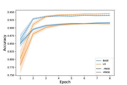
Figure 2 is the training curve for the BERT models over ReLocaR. We find that, generally, BERT-lg converges a bit slower than BERT-base, but in each case, the masked model performs substantially better than the unmasked models, and is more data efficient. While we do not include them in the paper, the plots for other datasets showed a similar trend.


6 Error Analysis
To further understand the task of metonymy resolution and why the model fails in some cases, we conducted a manual error analysis over a random sample of 150 errors from SemEval and ReLocaR. We roughly categorise the errors into 6 types, with each instance classified according to a unique error type. Some instances had multiple errors among types 4, 5, and 6, in which case we classified them in the priority of .
-
1.
Data quality: Although the two datasets are labeled by experts, the inter-annotator agreement is not perfect, and the annotation guidlines are not exactly the same. For example, location-for-government is literal in SemEval but metonymic in ReLocaR. Even based on the annotation guidelines used to generate the datasets, there are some labels that we do not agree with, such as the example for Type 1 in Table 6: in our judgement, England is the literal place or country here, but the gold label is metonym.
-
2.
Insufficient context: Due to model capacity and efficiency reasons, we restrict the context to the context sentence of the PMWs. This removes useful context in some cases, such as the example for Type 2 in Table 6, where the preceding sentence is: He will forsake China production schedules for fine tuning the first of many travel itineraries planned for “my new career of retirement”, as he put it. With this context, it is easier to recognise the PMW Canada as an event, and hence a metonym. These errors can be resolved by including more context.
-
3.
Mixed meaning: Some PMWs have both a literal and metonymic reading. We follow ?) in treating them as metonymies, but the dominant reading is sometimes literal. In the example for Type 3 in Table 6, Malaysia can either be the geographic place or the government of Malaysia. Such errors can be better handled with a more fine-grained classification schema.
-
4.
Long distance implications or complex syntactic structure: The models struggle when the sentence structure becomes complex. For example, in the example for Type 4 in Table 6, the immediate context suggests the PMW is literal, but the broader context suggests the opposite. Such issues can be addressed by using models with richer representations of sentence structure.
-
5.
Misleading wording and complex sentence semantics: Complex semantics and grammatical phenomena like noun possessives confuse the model. America in the phrase America’s nuclear stockpile has the literal reading, while Lebanon in the phrase Lebanon’s long ordeal has a metonymic reading. A particularly subtle example is that for Type 5 in Table 6, which requires the model to have near-human comprehension of semantics.
-
6.
Missing world knowledge: Some examples require background knowledge to be understood, such as the example for Type 6 in Table 6, where Vietnam refers to an event (a war that happened there, and Bill Clinton’s actions related to that war777https://en.wikipedia.org/wiki/Bill_Clinton#Vietnam_War_opposition_and_draft_controversy). To deal with this, the model needs to have access to world knowledge, either implicitly or explicitly.
These 6 error types vary in difficulty. From Table 6, we see that 62% of current errors are caused by Types 5–6, namely the model lacking an understanding of complex sentence semantics or world knowledge, which are hard to solve. Possibly the only case with a clear resolution is Type 2, where larger-context models may perform better.
| Type | Example | Label | Rate |
|---|---|---|---|
| 1 | Jordan Houghton is a youth football player who plays in the England national under-17 football team. | metonymy | 5% |
| 2 | Canada in the Spring is already planned and Roy and his wife, Ann, are finalising the details of what promises to be an exciting six-week sojourn | metonymy | 12% |
| 3 | The role of this office is to supply and coordinate aid from Malaysia to Kosovo and also to enable communication between the Malaysian government and the UNMIK. | metonymy | 8% |
| 4 | Western Australia becomes the last Australian state to abolish capital punishment for ordinary crimes (i.e., murder). | metonymy | 8% |
| 5 | Yet, although Britain suffered severe economic depression and rising unemployment, her economic plight was much less marked than that of Germany and Italy. | literal | 44% |
| 6 | Sex, drugs and Vietnam have haunted Bill Clinton’s campaign for the US presidency. | metonymy | 23% |
7 Conclusions and Future Work
In this paper, we proposed a word masking approach to metonymy resolution based on pre-trained BERT, which substantially outperforms existing methods over a broad range of datasets. We also evaluated the ability of different models in a cross-domain setting, and showed our proposed method to generalise the best. We further demonstrated that an end-to-end metonymy resolution model can improve the performance of a downstream geoparsing task, and conducted a systematic error analysis of our model.
The proposed target word masking method can be applied to tasks beyond metonymy resolution. Numerous word-level classification tasks lack large-scale, high-quality, balanced datasets. We plan to apply the proposed word masking approach to these tasks to investigate whether it can lead to similar gains over other tasks.
8 Acknowledgements
This research was sponsored in part by the Australian Research Council. The authors would like to thank the anonymous reviewers for their insightful comments.
References
- [Brun et al. (2007] Caroline Brun, Maud Ehrmann, and Guillaume Jacquet. 2007. XRCE-m: A hybrid system for named entity metonymy resolution. In Proceedings of the Fourth International Workshop on Semantic Evaluations, pages 488–491, Prague, Czech Republic.
- [Devlin et al. (2019] Jacob Devlin, Ming-Wei Chang, Kenton Lee, and Kristina Toutanova. 2019. BERT: Pre-training of deep bidirectional transformers for language understanding. In Proceedings of the 2019 Conference of the North American Chapter of the Association for Computational Linguistics, pages 4171–4186, Minneapolis, USA.
- [Farkas et al. (2007] Richárd Farkas, Eszter Simon, György Szarvas, and Dániel Varga. 2007. GYDER: Maxent metonymy resolution. In Proceedings of the Fourth International Workshop on Semantic Evaluations, pages 161–164, Prague, Czech Republic.
- [Fass (1991] Dan Fass. 1991. met*: A method for discriminating metonymy and metaphor by computer. Computational Linguistics, 17(1):49–90.
- [Gritta et al. (2017] Milan Gritta, Mohammad Taher Pilehvar, Nut Limsopatham, and Nigel Collier. 2017. Vancouver welcomes you! Minimalist location metonymy resolution. In Proceedings of the 55th Annual Meeting of the Association for Computational Linguistics, pages 1248–1259, Vancouver, Canada.
- [Gritta et al. (2018] Milan Gritta, Mohammad Taher Pilehvar, Nut Limsopatham, and Nigel Collier. 2018. What’s missing in geographical parsing? Language Resources and Evaluation, 52(2):603–623.
- [Gritta et al. (2019] Milan Gritta, Mohammad Taher Pilehvar, and Nigel Collier. 2019. A pragmatic guide to geoparsing evaluation. Language Resources and Evaluation.
- [Grover et al. (2010] Claire Grover, Richard Tobin, Kate Byrne, Matthew Woollard, James Reid, Stuart Dunn, and Julian Ball. 2010. Use of the Edinburgh geoparser for georeferencing digitized historical collections. Philosophical Transactions of the Royal Society A: Mathematical, Physical and Engineering Sciences, 368(1925):3875–3889.
- [Hobbs et al. (1993] Jerry R Hobbs, Mark E Stickel, Douglas E Appelt, and Paul Martin. 1993. Interpretation as abduction. Artificial Intelligence, 63(1-2):69–142.
- [Hobbs Sr and Martin (1987] Jerry R Hobbs Sr and Paul Martin. 1987. Local pragmatics. Technical report, SRI International Menlo Park CA Artificial Intelligence Center.
- [Houlsby et al. (2019] Neil Houlsby, Andrei Giurgiu, Stanislaw Jastrzkebski, Bruna Morrone, Quentin de Laroussilhe, Andrea Gesmundo, Mona Attariyan, and Sylvain Gelly. 2019. Parameter-efficient transfer learning for NLP. In Proceedings of the 36th International Conference on Machine Learning, pages 2790–2799, California, USA.
- [Kamei and Wakao (1992] Shin-ichiro Kamei and Takahiro Wakao. 1992. Metonymy: Reassessment, survey of acceptability, and its treatment in a machine translation system. In Proceedings of the 30th Annual Meeting of the Association for Computational Linguistics, pages 309–311, Newark, USA.
- [Kevin and Michael (2020] Alex Mathews Kevin and Strube Michael. 2020. A large harvested corpus of location metonymy. In Proceedings of the 12th Edition of Language Resources and Evaluation Conference, Marseille, France.
- [Kobayashi (2018] Sosuke Kobayashi. 2018. Contextual augmentation: Data augmentation by words with paradigmatic relations. In Proceedings of the 2018 Conference of the North American Chapter of the Association for Computational Linguistics: Human Language Technologies, pages 452–457, New Orleans, USA.
- [Leveling and Hartrumpf (2008] Johannes Leveling and Sven Hartrumpf. 2008. On metonymy recognition for geographic information retrieval. International Journal of Geographical Information Science, 22(3):289–299.
- [Levy et al. (2015] Omer Levy, Steffen Remus, Chris Biemann, and Ido Dagan. 2015. Do supervised distributional methods really learn lexical inference relations? In Proceedings of the 2015 Conference of the North American Chapter of the Association for Computational Linguistics: Human Language Technologies, pages 970–976, Denver, USA.
- [Markert and Hahn (2002] Katja Markert and Udo Hahn. 2002. Understanding metonymies in discourse. Artificial Intelligence, 135(1-2):145–198.
- [Markert and Nissim (2002] Katja Markert and Malvina Nissim. 2002. Metonymy resolution as a classification task. In Proceedings of the 2002 Conference on Empirical Methods in Natural Language Processing, pages 204–213, Philadelphia, USA.
- [Markert and Nissim (2007] Katja Markert and Malvina Nissim. 2007. SemEval-2007 task 08: Metonymy resolution at SemEval-2007. In Proceedings of the Fourth International Workshop on Semantic Evaluations, pages 36–41, Prague, Czech Republic.
- [Markert and Nissim (2009] Katja Markert and Malvina Nissim. 2009. Data and models for metonymy resolution. Language Resources and Evaluation, 43(2):123–138.
- [Monteiro et al. (2016] Bruno R. Monteiro, Clodoveu A. Davis Jr., and Frederico T. Fonseca. 2016. A survey on the geographic scope of textual documents. Computational Geosciences, 96:23–34.
- [Nastase and Strube (2009] Vivi Nastase and Michael Strube. 2009. Combining collocations, lexical and encyclopedic knowledge for metonymy resolution. In Proceedings of the 2009 Conference on Empirical Methods in Natural Language Processing, pages 910–918, Singapore.
- [Nastase and Strube (2013] Vivi Nastase and Michael Strube. 2013. Transforming Wikipedia into a large scale multilingual concept network. Artificial Intelligence, 194:62–85.
- [Nastase et al. (2012] Vivi Nastase, Alex Judea, Katja Markert, and Michael Strube. 2012. Local and global context for supervised and unsupervised metonymy resolution. In Proceedings of the 2012 Joint Conference on Empirical Methods in Natural Language Processing and Computational Natural Language Learning, pages 183–193, Jeju Island, Korea.
- [Nicolae et al. (2007] Cristina Nicolae, Gabriel Nicolae, and Sanda Harabagiu. 2007. UTD-HLT-CG: Semantic architecture for metonymy resolution and classification of nominal relations. In Proceedings of the Fourth International Workshop on Semantic Evaluations, pages 454–459, Prague, Czech Republic.
- [Nissim and Markert (2003] Malvina Nissim and Katja Markert. 2003. Syntactic features and word similarity for supervised metonymy resolution. In Proceedings of the 41st Annual Meeting of the Association for Computational Linguistics, pages 56–63, Sapporo, Japan.
- [Pennington et al. (2014] Jeffrey Pennington, Richard Socher, and Christopher Manning. 2014. GloVe: Global vectors for word representation. In Proceedings of the 2014 Conference on Empirical Methods in Natural Language Processing (EMNLP 2014), pages 1532–1543, Doha, Qatar.
- [Peters et al. (2018] Matthew Peters, Mark Neumann, Mohit Iyyer, Matt Gardner, Christopher Clark, Kenton Lee, and Luke Zettlemoyer. 2018. Deep contextualized word representations. In Proceedings of the 2018 Conference of the North American Chapter of the Association for Computational Linguistics: Human Language Technologies, pages 2227–2237, New Orleans, USA.
- [Porada et al. (2019] Ian Porada, Kaheer Suleman, and Jackie Chi Kit Cheung. 2019. Can a gorilla ride a camel? Learning semantic plausibility from text. In Proceedings of the First Workshop on Commonsense Inference in Natural Language Processing, pages 123–129, Hong Kong, China.
- [Pustejovsky (1991] James Pustejovsky. 1991. The generative lexicon. Computational Linguistics, 17(4):409–441.
- [Stallard (1993] David Stallard. 1993. Two kinds of metonymy. In Proceedings of the 31st Annual Meeting of the Association for Computational Linguistics, pages 87–94, Columbus, USA.
- [Vylomova et al. (2016] Ekaterina Vylomova, Laura Rimell, Trevor Cohn, and Timothy Baldwin. 2016. Take and took, gaggle and goose, book and read: Evaluating the utility of vector differences for lexical relation learning. In Proceedings of the 54th Annual Meeting of the Association for Computational Linguistics (ACL 2016), pages 1671–1682, Berlin, Germany.
- [Wei and Zou (2019] Jason Wei and Kai Zou. 2019. EDA: Easy data augmentation techniques for boosting performance on text classification tasks. In Proceedings of the 2019 Conference on Empirical Methods in Natural Language Processing and the 9th International Joint Conference on Natural Language Processing, pages 6381–6387, Hong Kong, China.