Takagi Topological Insulator on the Honeycomb Lattice
Abstract
Recently, real topological phases protected by symmetry have been actively investigated. In two dimensions, the corresponding topological invariant is the Stiefel-Whitney number. A recent theoretical advance is that in the presence of the sublattice symmetry, the Stiefel-Whitney number can be equivalently formulated in terms of Takagi’s factorization. The topological invariant gives rise to a novel second-order topological insulator with odd -related pairs of corner zero modes. In this article, we review the elements of this novel second-order topological insulator, and demonstrate the essential physics by a simple model on the honeycomb lattice.
Introduction. The symmetry-protected topological phases, such as topological (crystalline) insulators (TIs) and superconductors (TSCs), have been one of the most active fields of physics during the last fifteen years Volovik (2003); Hasan and Kane (2010); Qi and Zhang (2011); Fu (2011); Chiu et al. (2016); Kruthoff et al. (2017); Benalcazar et al. (2017); Liu et al. (2019); Xie et al. (2021). Based on the topological theory, the topological band theory has been established to classify and characterize various topological states Atiyah (1966); Kitaev (2010); Schnyder et al. (2008). Symmetry plays an fundamental role in the classification of topological phases. Considering three discrete symmetries, namely time reversal , charge conjugation and chiral symmetry , physical systems can be classified into ten symmetry classes, termed Altland-Zirnbauer (AZ) classes Altland and Zirnbauer (1997); Kitaev (2010); Hořava (2005); Atiyah (1966); Schnyder et al. (2008); Zhao and Wang (2014), among which the eight ones with at least or are called real AZ classes. The topological classifications in the framework of the eight real AZ classes correspond to the real theory. Using the real theory, gapped systems including topological insulators and topological superconductors were first classified Schnyder et al. (2008); Kitaev (2010); Ryu et al. (2010), and then gapless systems were classified as well Matsuura et al. (2013); Zhao and Wang (2013); Chiu and Schnyder (2014); Shiozaki and Sato (2014). All the classification tables exhibit an elegant eightfold periodicity along the dimensions for the eight real AZ classes.
After internal symmetries like and , more and more spatial symmetries were involved to enrich symmetry-protected topological matter. It was noticed that combined symmetries and correspond to the orthogonal theory with the spatial inversion, since they leave every point fixed in the reciprocal space. Hence, the topological classification table was worked out Zhao et al. (2016). A remarkable feature is that groups , and in the table appear in the reversed order in dimensionality, compared with previous tables for the real AZ classes. and are fundamental in nature, and therefore the classification table has been applied to explore topological phases in various physical systems, such as quantum materials Zhao and Lu (2017); Kruthoff et al. (2017); Ahn et al. (2019), topological superconductors Timm et al. (2017); Yu et al. (2021); Tomonaga et al. (2021); Lapp et al. (2020), and photonic/phononic crystals and electric-circuit arrays Zhang et al. (2013); Yang et al. (2015); Imhof et al. (2018); Ozawa et al. (2019); Ma et al. (2019); Serra-Garcia et al. (2018); Yu et al. (2020); Peterson et al. (2018); Lapp et al. (2020), and can generate unique topological structures with many novel consequences, such as non-Abelian topological charges, cross-order boundary transitions, and nodal-loop linking structures Zhao and Lu (2017); Yu et al. (2015); Ahn et al. (2019); Sheng et al. (2019); Wu et al. (2019); Wang et al. (2019); Li et al. (2020).
Remarkably, from the classification table, the symmetry class with corresponds to the classification for and . As revealed in Ref.Zhao and Lu (2017), leads to real band structures in contrast to conventional complex band structures. Then, the topological invariant for can be formulated as the quantized Berry phase in units of modulo . The case of is much fascinating. The topological invariant is the Euler number, a real version of the Chern number, for two valence bands. The Euler number is valued in , but only its parity is stable if more trivial valence bands are added into consideration. The parity, namely the Euler number modulo , is just the Stiefel-Whitney number in two dimensions, which determines whether the real vector bundle can be lifted into a spinor bundle.
The topological invariant gives rise to novel topological phases with extraordinary properties. In D, it characterizes a real Dirac semimetal, which can be transformed into a nodal ring with symmetry-preserving perturbations. Then, the nodal ring is characterized by two topological charges . In D, it describes a topological insulator. The common topological wisdom is that the bulk topological invariant determines a unique form of the boundary modes, namely the well-known one-to-one bulk-boundary correspondence. However, a remarkably discovery in Ref.Wang et al. (2020) is that corresponds to multiple forms of boundary modes, extending the one-to-one correspondence to one-to-many. The D topological insulator can host various second-order phases with odd -related pairs of corner zero-modes, which are mediated by first-order phases with helical edge states. Similarly, the D semimetal can host second-order hinge Fermi arcs and first-order surface Dirac states as well. Recently, graphynes have been proposed as the material candidates which can realize both the D topological insuslator and the D topological semimetal Sheng et al. (2019); Chen et al. (2021, 2022).
As aforementioned, the second-order phases of the D topological insulator feature odd -related pairs of corner zero modes. It is interesting to look for its D analog, which has been presented in Ref.Dai et al. (2021). Referring to the topological classification table for and symmetries, we notice that although the classification for is trivial, with an additional chiral symmetry with the classification is preserved as in D and, more importantly, becomes nontrivial as in D. It is found that the corresponding topological invariants can be formulated in terms of Takagi’s factorization. The topological invariant in D is equivalent to , while that in D is a new topological invariant. Either in D or in D the bulk topological invariant can be manifested as odd -related pairs of corner zero-modes. Now, with the chiral symmetry, the two zero-modes in each pair are eigenstates with opposite eigenvalues of the chiral symmetry.
In this article, we review the elements of D -protected topological insulators with or without chiral symmetry. The essential physics is demonstrated by the Honeycomb-lattice model, with only the nearest-neighbor hopping amplitudes. We show that under certain dimerization patterns the model is a topological insulator with nontrivial Stiefel-Whitney number or the Takagi topological invariant, and therefore presents all the nontrivial topological phenomena. Particularly, under various -invariant geometries, there are always odd -related pairs of corner zero-modes for the second-order topological phase. Before diving into the details, it is noteworthy that the dimerized honeycomb model can be regarded as an abstraction from the graphynes Sheng et al. (2019); Chen et al. (2021, 2022).
The honeycomb-lattice model.
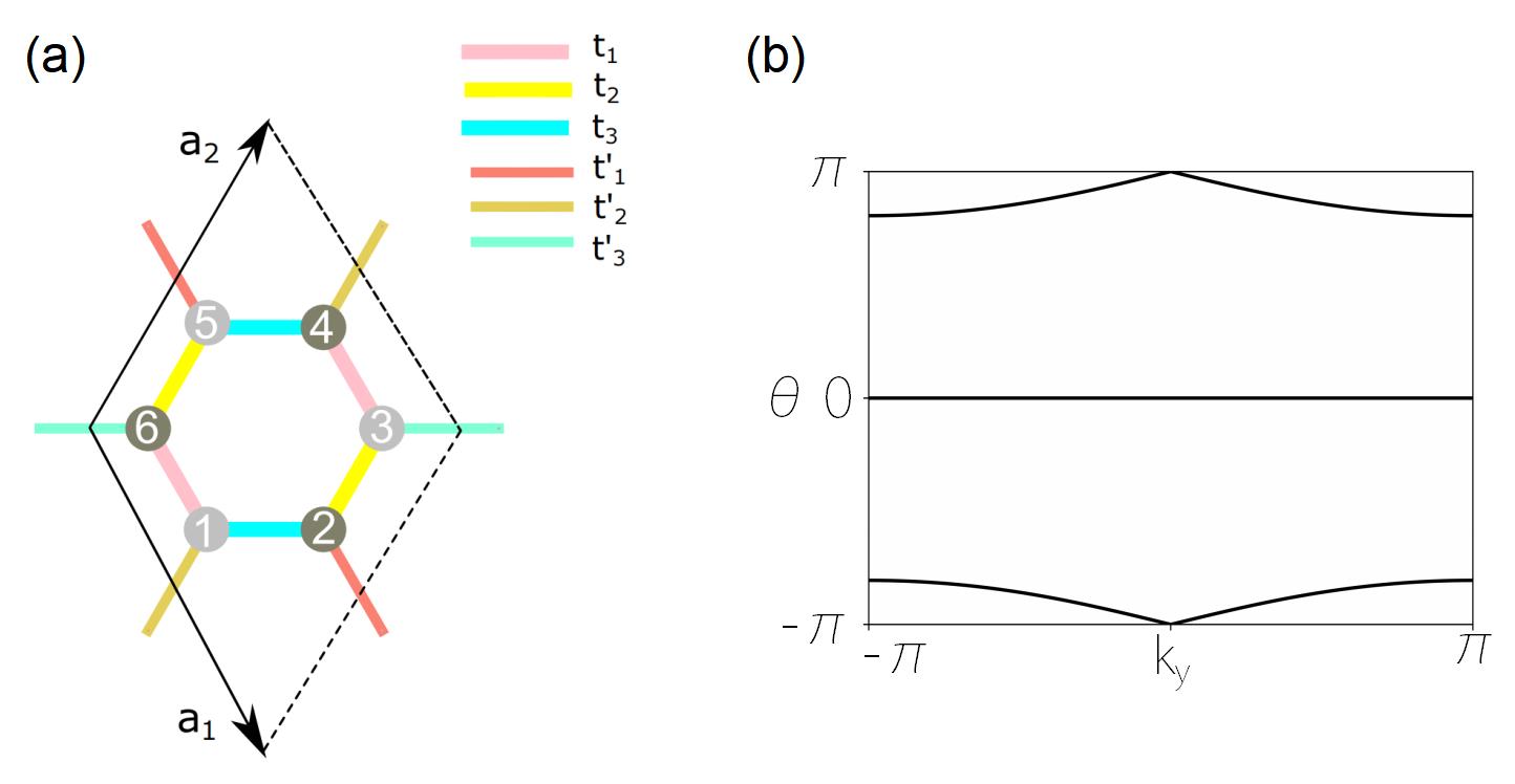
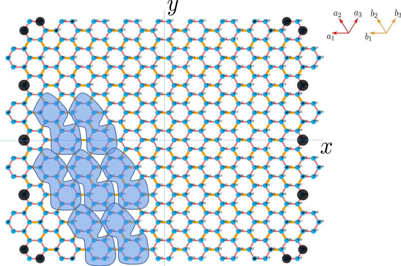
Let us start with presenting the honeycomb-lattice model, the lattice structure is shown in Fig. 1(a). The Hamiltonian in momentum space is given by
| (1) |
where with . Here, are the bond vectors connecting the centers of nearest-neighbor unit cells, as indicated in Fig.1(a) with . The Hamiltonian has inversion symmetry with , spinless time-reversal symmetry with , and therefore spacetime-inversion symmetry with , where is the complex conjugation and is the inversion of momenta. Note that ’s are the Pauli matrices acting on the sublattice space [see Fig.1(a)], and is the identity matrix. Each inversion center is taken as the center of a hexagon in real space. The sublattice symmetry operator is . Since the inversion exchanges sublattices, both and anti-commute with , namely, .
To obtain the nontrivial topological phases, we calculate the determinant of the Hamiltonian (1) at point Gam in the Brillouin zone as
| (2) |
Since the bulk topological criticality generally corresponds gap-closing point, we can obtain the topological phase-transition points by letting , which gives
| (3) |
Interestingly, if (3) holds, the system is generally reduced to a topologically equivalent graphene model with two Dirac points in the first Brillouin zone Haldane (1988). When , the system steps into a topological phase, while conversely the system becomes a trivial phase, which can be checked by computing Stiefel-Whitney number or Takagi’s factorization.
Topological invariants The topology can be determined by various formulas of the topological invariant. We now briefly review them. First, as given in Ref.Zhao and Lu (2017), the topological invariant can be determined by the Wilson loop
| (4) |
(with indicating the path order) along large circles parametrized by . is the contour at a fixed and is the non-Abelian Berry connection for the valence bands. The topological information is encoded in the phase factors of the eigenvalues of for valence bands:
| (5) |
Different from the conventional TIs and Chern insulators, the Wilson loop spectral flow for real phases are mirror symmetric with respect to the axis [see Fig. 1(b)]. This is because is equivalent to a mapping from to up to a unitary transformation Zhao and Lu (2017). The topological information can be pictorially derived from counting how many times the trajectories cross as
| (6) |
For honeycomb lattice with , a single crossing exsit as shown in Fig.1(b), namely, , which indicates the model is in a topological nontrivial phase.
As aforementioned, our system is protected by spacetime inversion symmetry and sublattice (chiral) symmetry . These symmetries constraint the classifying space of to be symmeric unitary matrices. Thus the invariant from the Takagi’s factorization can be defined Dai et al. (2021), which leads to an alternative formulation for . We now prove the equivalence of the two formulas. For technical simplicity, we assume the momentum space as a sphere , which is sufficient to present the essential ideas.
In general, requires the Hamiltonian to be block anti-diagonal and requires the upper-right block to be symmetric. Thus the flattened Hamiltonian is given by
| (7) |
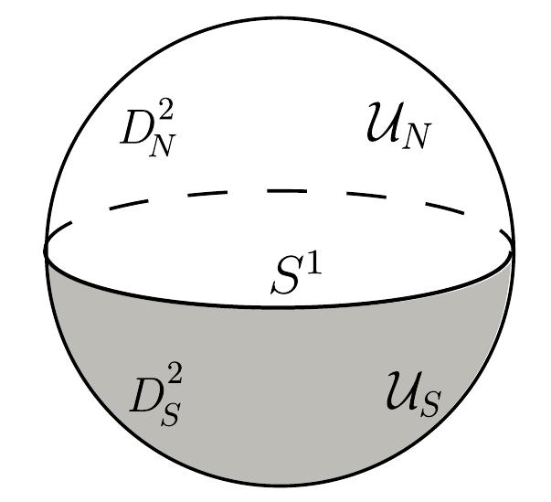
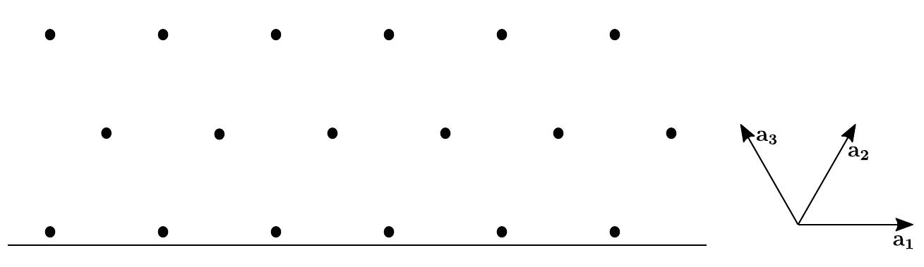
where is a unitary symmetric matrix for each and denotes the number of valence (conduction) bands. is the Takagi factor. The classifying space for this symmetric class is Dai et al. (2021). Here, corresponds to the topological invariant of our system. Consider a D sphere , which is divided into north and south hemispheres , overlapping along the equator . The Takagi factors over , respectively, can be transformed to each other by a gauge transformation over the equator , as shown in Fig. 2. is given by
for leads to obstructions for a global Takagi’s factorization over .
The conduction and valence wavefunctions of can be given by
| (8) |
where . is a unit vector with “” locating at the -th position.
Performing a unitary transformation on this system, the Hamiltonian and valence wavefunctions both become real. Meanwhile, and are transformed to and , respectively. Over the intersection , transition function of real valence wavefunctions can be given by
| (9) |
Thus, we know the transition function of real valence wavefunctions is equal to the gauge transformation . As noted in Ref.Zhao and Lu (2017), is just the parity of the winding number of the transition function for valence bands. Thus, we see the equivalence of two D topological invariants.
Physical consequence. According to analytical and numerical methods, we reveal that three pairs of hopping parameters and (with ) jointly determine the configuration of topological boundary modes. To facilitate understanding the relation between distinct boundary modes and parameters, we define a boundary effective mass term for each edge:
| (10) |
where the subscript denotes the hopping along the primitive vector direction (). The above Eq.(10) can be derived from the boundary effective Hamiltonian Edg . Hence, if , the corresponding edges are gapless, which is also the boundary critical condition to separate two second-order topological phases.
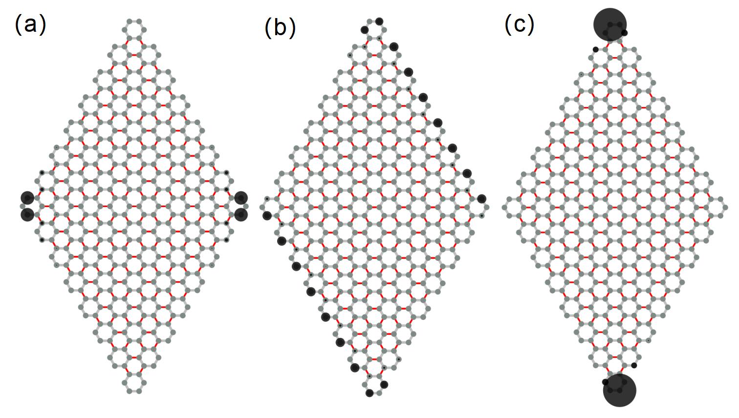
To demonstate the boundary modes, we consider a rhombic-shaped D sample with armchair termination, i.e., by opening boundary along and direction, as shown in Fig. 3. If and , the helical edge modes along periodic can be obtained, as shown in Fig. 3(b). However, once , the helical edge modes will be gapped and the localized corner modes will emerge. More specifically, for the case with (), the corner modes will locate at () corners, as shown in Fig.3(a) and (c) respectively. The symmetry requires that the corner zero-modes always come in pairs and the chiral symmetry sets the midgap modes exactly at zero energy Fin .
To keep the completeness of honeycomb unit cell in a rhomboid sample, one only has three kinds of armchair edges, namely the edge parallel to direction with . If the edge connected by the same corner has the same mass term sign, the corner zero-modes will be localized at the obtuse angle of the rhomboid, otherwise at acute corners. We shall theoretically explain these numerical results in the next section. It is emphasized that in the whole process of the edge-phase transitions, the bulk gap is always open and the symmetries are preserved, therefore, the bulk invariant is unchanged. Thus the conventional bulk-boundary correspondence is not appliable for TTI, namely, the bulk invariant can not uniquely determine the boundary modes, but dictates an edge criticality, as the concept mentioned in previous work Wang et al. (2020).
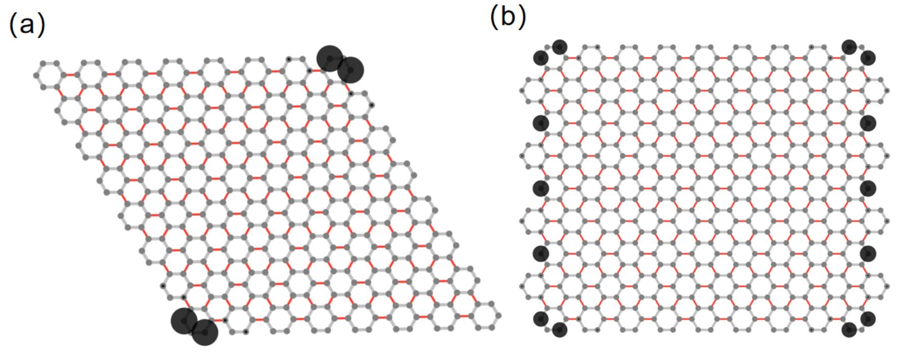
As promised in introduction, we now proceed to tune the boundary modes with fixed parameters. In the rhombic case, all samples terminate with armchair edges and exhibit parameter-depended boundary modes. As long as and are not violated, the finite samples can be cut with not only rhomb as shown in Fig. 3, but also hexagon(see Fig.5 ). Beside armchair edges, zigzag edges can serve as termination too. Creatively, with fixed parameters but different boundary selections, one can also find various distinguishable boundary modes. For instance, helical edge states emerge on the zigzag edges in a rectangle sample as shown in Fig. 4(b), with the same hopping parameters as Fig. 4(a). This result further proves that the bulk topological invariant can not uniquely determine the topological boundary modes. We also study lots of other patterns with the same parameters, and abundant topological boundary modes consisting of corner zero modes and gapless edge modes can be obtained (see Appendix. D). They are all boundary-selection-depended. Hence, we propose that one can obtain needed topological boundary modes by choosing particular boundary geometry, without tuning parameters, which is usually difficult to perform in real systems.
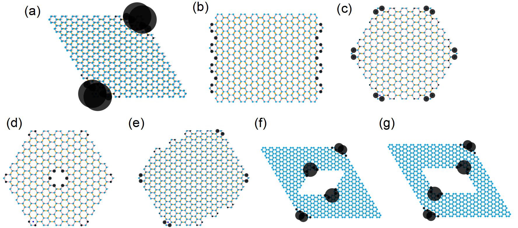
Novelly, in both situations discussed above, for second-order topological phases, the number of the zero-energy corners must be odd pairs. For example, for a hexagonal sample, we can only find one or three pairs of zero-mode corners, as shown in Fig. 5(a) and (b). Similarly, the Octagonal sample also has one or three pairs of zero-mode corners as shown in Fig. 5(c) and (d).
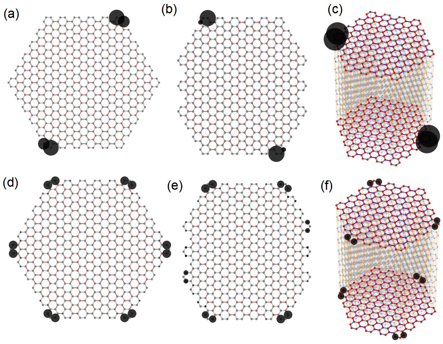
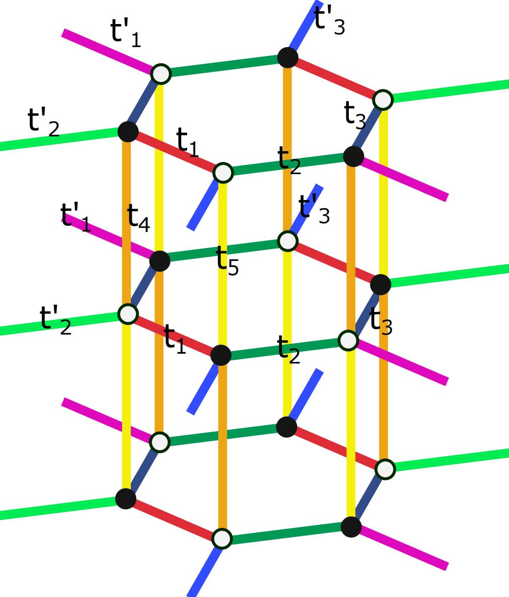
We find that the peculiarity of odd-pair-zero-modes is universal and it can be generalized to a higher-dimensional situation, such as 3D Dai et al. (2021). The 3D model is constructed by stacking the 2D honeycomb TTI discussed above in a staggered manner to preserve the sublattice symmetry . The details of the construction of the model can be found in Appendix. C . The inversion center is chosen as the center of hexagonal in one layer. Thus the anti-commuting relation of and are preserved. We cut a finite hexagonal prisms sample that keeps the symmetries. One can find only odd pairs (one or three) of corner states related by appear. Note that the corner zero-modes can be driven to other corners by tunning the hopping parameters like in a 2D situation.
Analytic method. We first proceed to solve the boundary criticality along the periodic direction and openning boundary with . Replace by in Hamiltonian (1), with ladder operator and . Then can be represented by since . After a series of tedious derivation (see Appendix. A), we obtian the effective Hamiltonian of the bottom boundary:
| (11) |
Following the same argument with aforementioned bulk criticality, we can obtain the boundary criticality by letting , which leads to
| (12) |
The above Eq. (12) holds only at . Thus, when the system is in a topological nontrivial case, Eq. (12) related edge criticality separates two different second-order topological phases with corner zero modes. Likely, we can obtain similar results for periodic and directions. For convenience, we can define boundary effective mass by the left of Eq. (12) for edges parallel to . Or, generally Eq. (10) for edges parallel to . Different from the armchair edges, the zigzag terminations has an additional boundary criticality, namely, the effective masses can be defined by
| (13) |
The derived details can be found in the Appendix. B.
With the effective mass orderly distributing on each edge Edg , the existence of corner zero-modes is reduced to a Jackiw-Rebbi problem Jackiw and Rebbi (1976). The corners with opposite effective masses on both sides can have zero-modes.
Discussion. In this article, we present a simple 2D realizable honeycomb-lattice model to demonstrate the essential physics of the Takagi topological insulator. It is found that with unchanged topological invariant, one can tune topological boundary modes by not only parameters, but also boundary selections. It goes beyond the common wisdom about bulk-boundary correspondence, and gives rise to much richer boundary physics.
Our model with novel physics is closely related to real systems. It is easier to realize our model by photonic/phononic crystals, electric-circuit arrays and mechanics systems, since only have nearest-neighbor hopping amplitudes are included into the model. Several special cases of our model have been recently realized in photonic/phononic crystals Yang et al. (2020); Noh et al. (2018), where hopefully the general form of our model can be further experimentally examined.
Acknowledgements.
The authors acknowledge the support from the National Natural Science Foundation of China under Grants (No.11874201, No.12174181, and No.12161160315).Appendix A Theoretical method for critical conditon of rhombic sample
The lattice is shown as FIG.1 in main text. The Hamiltonian in D momentum space is given in Eq. (1). The determinant of is given as
For simplicity, we write as . To make gapless, we obtain
| (14) |
Because the hopping terms are real and positive, we know that
| (15) |
with . Meanwhile, the second formula in the Eq. (14) always holds. Therefore, corresponds to the gapless phase, which is also the critical phase between trival and nontrival phases.
Opening the boundary parallel to the lattice vector as FIG. 6, the Hamiltonian is transformed to
where and are the forward and backward translation operators along the -direction, respectively. The actions of and on the real space basis of the tight-binding model for the the -direction are given by
| (16) |
where the nonnegative integer i labeling the lattice site along the -direction. Accordingly, the matrices can be explicitly written as
Adopting the Anstze
with for the boundary states. In the bulk with , we obtain that
| (17) |
Restricting to the surface layer with , we obtain that
| (18) |
The difference of Eqs. (17) and (18) gives . Thus, the effective Hamiltonian for the boundary state is
| (19) |
The determinant of is given by
| (20) |
Therefore, we know with only when . In other words, the boundary effective Hamiltonian corresponds to a gapless phase only if . By the same way, we obtain the gapless boundary along the direction of and with and , respectively.
Appendix B Theoretical method for critical conditon of square-shaped sample
Here, we present the square-shaped and parallelogram-shaped boundary conditions as examples to derive the critical points for parameters.
The Hamiltonian in reciprocal space can be written as
To find the critical condition for topological phase transition, we calculate the determinant of the bulk Hamiltonian,
So, if the Hamiltonian has zero energy, det must be zero and
| (21) |
On the other hand,
| (22) |
if and only if , the equal sign establishes in the inequality. And at this moment, also holds. Hence the condition of det is
| (23) |
When the above equation holds, there exist gapless bulk states, more explicitly, there is a Dirac point localized at . So this condition may be the critical point between trivial and nontrivial topological phases. We check the parameter condition (23) with numerical wilson loop method and find the condition (23) is the critical point exactly.
Note that although the Eqs. (21) has solutions beyond point, such as , we check that the parameters conditions for these zero-energy points do not distingush the trivial and non-trivial topological phases.
B.1 The zigzag boundary
We first study zigzag boundary, namely, direction is periodic. In this case, by replacing with , where is ladder operator and . More explicitly, the semi-infinite translation operators are now written as
By taking the ansatz
| (24) |
for the boundary states, we solve the eigenvalue equation of Hamiltonian. In the bulk with , we have
| (25) |
On the boundary with , we have
| (26) |
The difference of Eqs. (25) and (26) gives
| (27) |
Since the boundary effective Hamiltonian is given by
| (28) |
we obtain the equivalent form of boundary effective Hamiltonian, namely, by deleting the rows and columns of the original Hamiltonian,
| (29) |
Since the topological transitions must undergo a gapless state (or break symmetries, but we preserve symmetries here), we can derive the critical conditons of phase-transition point by letting the determinant of being equal to , namely,
| (30) |
if and only if , the first equal sign establishes in the first inequality. And if and only if and , the second equal sign establishes in the second inequlity. Hence the condition of det having solutions is
| (31) |
When the above equation holds, there exist gapless boundary states along the zigzag boundary, more explicitly, there is a Dirac point localized at .
B.2 The armchair boundary
Following the same argument, we can obtain the boundary effective Hamiltonian along the periodic direction, namely, the armchair boundary,
| (32) |
Thus we have
| (33) |
if and only if , the first equal sign establishes in the first inequality. And if and only if and or , the second equal sign establishes in the second inequlity. However, the condition corresponds the trivial topological phases. Hence the condition of det having solutions is
| (34) |
It is noted that the relation is same as that of rohmbic sample. When the above equation holds, there exist gapless boundary states along the armchair boundary. More explicitly, there is a Dirac point localized at .
Appendix C 3D honeycomb model
We construct a 3D model by stacking 2D honeycomb Takagi insulator in a manner of stageer as shown in Fig.8. Here , the Hamiltonian is given by
| (35) |
where and
| (36) |
To get corner zero-modes of hexagonal prisms sample in main text, we set parameters as
Appendix D Different boundary modes
As proposed in maintext, by cutting different-shaped samples that preserve the symmetry, without changing the parameters, the system can possess distinguishable boundary-modes.
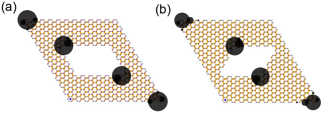
Here we take some representatived example to show that result, which can be seen in Fig.9 and 10. It is noted that, as shown in Fig.10, we can tune the position of corner zero-modes by cutting different gometric shape. Specificly, without changing parameters the local zero-modes can locate on different symmetry-related corners (acute angle or obtuse angle).
References
- Volovik (2003) G. E. Volovik, Universe in a helium droplet (Oxford University Press, Oxford UK, 2003).
- Hasan and Kane (2010) M. Z. Hasan and C. L. Kane, Rev. Mod. Phys. 82, 3045 (2010).
- Qi and Zhang (2011) X.-L. Qi and S.-C. Zhang, Rev. Mod. Phys. 83, 1057 (2011).
- Fu (2011) L. Fu, Phys. Rev. Lett. 106, 106802 (2011).
- Chiu et al. (2016) C.-K. Chiu, J. C. Y. Teo, A. P. Ascnyder, and S. Ryu, Rev. Mod. Phys. 88, 035005 (2016).
- Kruthoff et al. (2017) J. Kruthoff, J. de Boer, J. van Wezel, C. L. Kane, and R.-J. Slager, Phys. Rev. X 7, 041069 (2017).
- Benalcazar et al. (2017) W. A. Benalcazar, B. A. Bernevig, and T. L. Hughes, Phys. Rev. B 96, 245115 (2017).
- Liu et al. (2019) F. Liu, H.-Y. Deng, and K. Wakabayashi, Phys. Rev. Lett. 122, 086804 (2019).
- Xie et al. (2021) B. Xie, H.-X. Wang, X. Zhang, P. Zhan, J.-H. Jiang, M. Lu, and Y. Chen, Nat. Rev. Phys. 3, 520 (2021).
- Atiyah (1966) M. F. Atiyah, The Quarterly Journal of Mathematics 17, 367 (1966).
- Kitaev (2010) A. Kitaev, AIP Conference Proceedings 1134, 22 (2010).
- Schnyder et al. (2008) A. P. Schnyder, S. Ryu, A. Furusaki, and A. W. W. Ludwig, Phys. Rev. B 78, 195125 (2008).
- Altland and Zirnbauer (1997) A. Altland and M. R. Zirnbauer, Phys. Rev. B 55, 1142 (1997).
- Hořava (2005) P. Hořava, Phys. Rev. Lett. 95, 016405 (2005).
- Zhao and Wang (2014) Y. X. Zhao and Z. D. Wang, Phys. Rev. B 89, 075111 (2014).
- Ryu et al. (2010) S. Ryu, A. P. Schnyder, A. Furusaki, and A. W. W. Ludwig, New Journal of Physics 12, 065010 (2010).
- Matsuura et al. (2013) S. Matsuura, P.-Y. Chang, A. P. Schnyder, and S. Ryu, New Journal of Physics 15, 065001 (2013).
- Zhao and Wang (2013) Y. X. Zhao and Z. D. Wang, Phys. Rev. Lett. 110, 240404 (2013).
- Chiu and Schnyder (2014) C.-K. Chiu and A. P. Schnyder, Phys. Rev. B 90, 205136 (2014).
- Shiozaki and Sato (2014) K. Shiozaki and M. Sato, Phys. Rev. B 90, 165114 (2014).
- Zhao et al. (2016) X. Zhao, A. P. Schnyder, and Z. D. Wang, Phys. Rev. Lett. 116, 156402 (2016).
- Zhao and Lu (2017) Y. X. Zhao and Y. Lu, Phys. Rev. Lett. 118, 056401 (2017).
- Ahn et al. (2019) J. Ahn, S. Park, and B.-J. Yang, Phys. Rev. X (2019), 10.1103/PhysRevX.9.021013.
- Timm et al. (2017) C. Timm, A. P. Schnyder, D. F. Agterberg, and P. M. R. Brydon, Phys. Rev. B 96, 094526 (2017).
- Yu et al. (2021) T. Yu, D. M. Kennes, A. Rubio, and M. A. Sentef, Phys. Rev. Lett. 127, 127001 (2021).
- Tomonaga et al. (2021) A. Tomonaga, H. Mukai, F. Yoshihara, and J. S. Tsai, Phys. Rev. B 104, 224509 (2021).
- Lapp et al. (2020) C. J. Lapp, G. Börner, and C. Timm, Phys. Rev. B 101, 024505 (2020).
- Zhang et al. (2013) F. Zhang, C. L. Kane, and E. J. Mele, Phys. Rev. Lett. 110, 046404 (2013).
- Yang et al. (2015) Z. Yang, F. Gao, X. Shi, X. Lin, Z. Gao, Y. Chong, and B. Zhang, Phys. Rev. Lett. 114, 114301 (2015).
- Imhof et al. (2018) S. Imhof, C. Berger, F. Bayer, J. Brehm, L. W. Molenkamp, T. Kiessling, F. Schindler, C. H. Lee, M. Greiter, T. Neupert, and R. Thomale, Nature Physics 14, 925 (2018).
- Ozawa et al. (2019) T. Ozawa, H. M. Price, A. Amo, N. Goldman, M. Hafezi, L. Lu, M. C. Rechtsman, D. Schuster, J. Simon, O. Zilberberg, and I. Carusotto, Rev. Mod. Phys. 91, 015006 (2019).
- Ma et al. (2019) G. Ma, M. Xiao, and C. T. Chan, Nature Reviews Physics 1, 281 (2019).
- Serra-Garcia et al. (2018) M. Serra-Garcia, V. Peri, R. Süsstrunk, O. R. Bilal, T. Larsen, L. G. Villanueva, and S. D. Huber, Nature 555, 342 (2018).
- Yu et al. (2020) R. Yu, Y. X. Zhao, and A. P. Schnyder, National Science Review (2020), 10.1093/nsr/nwaa065.
- Peterson et al. (2018) C. W. Peterson, W. A. Benalcazar, T. L. Hughes, and G. Bahl, Nature 555, 346 (2018).
- Yu et al. (2015) R. Yu, H. Weng, Z. Fang, X. Dai, and X. Hu, Phys. Rev. Lett. 115, 036807 (2015).
- Sheng et al. (2019) X.-L. Sheng, C. Chen, H. Liu, Z. Chen, Z.-M. Yu, Y. X. Zhao, and S. A. Yang, Phys. Rev. Lett. 123, 256402 (2019).
- Wu et al. (2019) Q. Wu, A. A. Soluyanov, and T. Bzdušek, Science 365, 1273 (2019).
- Wang et al. (2019) Z. Wang, B. J. Wieder, J. Li, B. Yun, and B. A. Bernevig, Phys. Rev. Lett. 123, 186401 (2019).
- Li et al. (2020) H. Li, A. Mekawy, A. Krasnok, and A. Alù, Phys. Rev. Lett. 124, 193901 (2020).
- Wang et al. (2020) K. Wang, J.-X. Dai, L. B. Shao, S. A. Yang, and Y. X. Zhao, Phys. Rev. Lett. 125, 126403 (2020).
- Chen et al. (2021) C. Chen, W. Wu, Z.-M. Yu, Z. Chen, Y. X. Zhao, X.-L. Sheng, and S. A. Yang, Phys. Rev. B 104, 085205 (2021).
- Chen et al. (2022) C. Chen, X.-T. Zeng, Z. Chen, Y. X. Zhao, X.-L. Sheng, and S. A. Yang, Phys. Rev. Lett. 128, 026405 (2022).
- Dai et al. (2021) J.-X. Dai, K. Wang, S. A. Yang, and Y. X. Zhao, Phys. Rev. B 104, 165142 (2021).
- (45) By the numerical calculation of Wilson loop, one can easily check that only the algebra of parameters obtained at point is the real bulk criticality, while the others are not.
- Haldane (1988) F. D. M. Haldane, Phys. Rev. Lett. 61, 2015 (1988).
- (47) Note that a pair of opposite edges parallel to have opposite mass terms since symmetry inverses the effective mass.
- (48) Finite-size effects can split the degenerate zero modes and deviate them from zero to form a ingap corner modes, but the deviation is exponentially suppressed with the sample size.
- Jackiw and Rebbi (1976) R. Jackiw and C. Rebbi, Phys. Rev. D 13, 3398 (1976).
- Yang et al. (2020) Z.-Z. Yang, X. Li, Y.-Y. Peng, X.-Y. Zou, and J.-C. Cheng, Phys. Rev. Lett. 125, 255502 (2020).
- Noh et al. (2018) J. Noh, W. A. Benalcazar, S. Huang, M. J. Collins, K. P. Chen, T. L. Hughes, and M. C. Rechtsman, Nature Photon 12, 408–415 (2018).