Tackling Intertwined Data and Device Heterogeneities in Federated Learning with Unlimited Staleness
Abstract
Federated Learning (FL) can be affected by data and device heterogeneities, caused by clients’ different local data distributions and latencies in uploading model updates (i.e., staleness). Traditional schemes consider these heterogeneities as two separate and independent aspects, but this assumption is unrealistic in practical FL scenarios where these heterogeneities are intertwined. In these cases, traditional FL schemes are ineffective, and a better approach is to convert a stale model update into a unstale one. In this paper, we present a new FL framework that ensures the accuracy and computational efficiency of this conversion, hence effectively tackling the intertwined heterogeneities that may cause unlimited staleness in model updates. Our basic idea is to estimate the distributions of clients’ local training data from their uploaded stale model updates, and use these estimations to compute unstale client model updates. In this way, our approach does not require any auxiliary dataset nor the clients’ local models to be fully trained, and does not incur any additional computation or communication overhead at client devices. We compared our approach with the existing FL strategies on mainstream datasets and models, and showed that our approach can improve the trained model accuracy by up to 25% and reduce the number of required training epochs by up to 35%. Source codes can be found at: https://github.com/pittisl/FL-with-intertwined-heterogeneity.
1 Introduction
Federated Learning (FL) McMahan (2016) could be affected by both data and device heterogeneities. Data heterogeneity is the heterogeneity of non-i.i.d. data distributions on different clients, which make the aggregated global model biased and reduces model accuracy Konečný (2016); Zhao (2018). Device heterogeneity arises from clients’ variant latencies in uploading their local model updates to the server, due to their different local resource conditions (e.g., computing power, network link speed, etc). An intuitive solution to device heterogeneity is asynchronous FL, which does not wait for slow clients but updates the global model whenever having received a client update Xie and Gupta. (2019). In this case, if a slow client’s excessive latency is longer than a training epoch, it will use an outdated global model to compute its model update, which will be stale when aggregated at the server and affect model accuracy. To tackle staleness, weighted aggregation can be used to apply reduced weights on stale model updates Chen and Jin. (2019); Wang (2022).
Most existing work considers data and device heterogeneities as two separate and independent aspects in FL Zhou (2021). This assumption, however, is unrealistic in many FL scenarios where these two heterogeneities are intertwined: data in certain classes or with particular features may only be available at some slow clients. For example, in FL for hazard rescue Ahmed et al. (2020), only devices at hazard sites have crucial data about hazards, but they usually have limited connectivity or computing power to timely upload model updates. Similar situations could also happen in FL scenarios where data with high importance to model accuracy is scarce and hard to obtain, such as disease evaluation in smart health, where only few patients have severe symptoms but are very likely to report symptoms with long delays due to their worsening conditions Chen et al. (2017).
In these cases, if reduced weights are applied to stale model updates from slow clients, important knowledge in these updates will not be sufficiently learned and hence affects model accuracy. Instead, a better approach is to equally aggregate all model updates and convert a stale model update into a unstale one, but existing techniques for such conversion are limited to a small amount of staleness. For example, first-order compensation can be applied on the gradient delay Zheng et al. (2017), by assuming staleness in FL is smaller than one epoch to ignore all the high-order terms in the difference between stale and unstale model updates Zhou and Lv. (2021). However, in the aforementioned FL scenarios, it is common to witness excessive or even unlimited staleness, and our experiments in show that the compensation error will quickly increase with staleness.
To efficiently tackle the intertwined data and device heterogeneities with unlimited staleness, in this paper we present a new FL framework that uses gradient inversion at the server to convert stale model updates, by mimicking the local models’ gradients produced with their original training data Zhu and Han. (2019a). The server inversely computes the gradients from clients’ stale model updates to obtain an estimated distribution of clients’ training data, such that a model trained with the estimated data distribution will exhibit a similar loss surface as that of using clients’ original training data. The server uses such estimated data distributions to retrain the current global model, as estimations of clients’ unstale model updates. Compared to other model conversion methods, such as training an extra generative model Yang (2019) or optimizing input data with constraints Yin (2020), our approach has the following advantages:
-
•
Our approach retains the clients’ FL procedure to be unchanged, and hence does not incur any additional computation or communication overhead at client devices, which usually have weak capabilities in FL scenarios.
-
•
Our approach does not require any auxiliary dataset nor the clients’ local models to be fully trained, and can hence be widely applied to practical FL scenarios.
-
•
In our approach, the server will not be able to recover any original samples or labels of clients’ local training data. and it cannot produce any recognizable information about clients’ local data. Hence, our approach does not impair the clients’ data privacy.
We evaluated our proposed technique by comparing with the mainstream FL schemes on multiple datasets and models. Experiment results show that when tackling intertwined data and device heterogeneities with unlimited staleness, our technique can significantly improve the trained model accuracy by up to 25% and reduce the required amount of training epochs by up to 35%. Since clients in FL need to compute and upload model updates to the server in every training epoch, such reduction of training epochs largely reduces the computing and communication overhead at clients.
2 Background and Motivation
In this section, we present preliminary results that demonstrate the ineffectiveness of existing methods in tackling intertwined data and device heterogeneities, hence motivating our proposed approach using gradient inversion.

2.1 Tackling Intertwined Heterogeneities in FL
Most existing solutions to staleness in AFL are based on weighted aggregation Chen and Jin. (2019); Wang (2022); Chen (2020). For example, [7] suggests that a model update’s weight exponentially decays with its amount of staleness, and some others use different staleness metrics to decide model updates’ weights Wang (2022). Chen (2020) decides these weights based on a feature learning algorithm. These existing solutions, however, are improperly biased towards fast clients, and will hence affect the trained model’s accuracy when data and device heterogeneities in FL are intertwined, because they will miss important knowledge in slow clients’ model updates.
To show this, we conducted experiments using a real-world disaster image dataset Mouzannar et al. (2018), which contains 6k images of 5 disaster classes (e.g., fires and floods) with different levels of damage severity. In FL of 100 clients, we set data heterogeneity as that each client only contain samples in one data class, and set device heterogeneity as a staleness of 100 epochs on 15 clients with images of severe damage. When using this dataset to fine-tune a pre-trained ResNet18 model, results in Figure 1 show that staleness leads to large degradation of model accuracy, and weighted aggregation results in even lower accuracy than direct aggregation, because contributions from images of severe damage on stale clients are reduced by the weights111In synchronous FL, stale updates will be simply skipped, corresponding to applying zero weights on these updates. Hence, similar performance degradation is also expected for synchronous FL..
On the other hand, if we increase the contributions from stale clients by using larger weights, although the model accuracy on these images of severe damage will improve, the larger weights will amplify the impacts of errors contained in stale model updates and hence affect the model’s overall accuracy in other data classes. Detailed results can be found in Appendix B.
In practical scenarios such as natural disasters, such large or unlimited staleness is common due to interruptions in communication at disaster sites, and the staleness is too large for server to wait for any slow clients. The large performance degradation of weighted aggregation, then, motivates us to instead convert stale model updates to unstale ones.
The only existing work on such conversion, to our best knowledge, uses the first-order Taylor expansion to compensate for errors in stale model updates Zheng et al. (2017). For a stale update , the estimated unstale update is:
| (1) |
Since the Hessian matrix is difficult to compute for neural networks, it is approximated as
| (2) |
where is an empirical hyper parameter. However, this method can only applies to small amounts of staleness Zhou et al. (2021); Li et al. (2023a); Tian et al. (2021), in which the high-order terms in the Taylor expansion can be negligible. To verify this, we use the same experiment setting as above and vary the amount of staleness from 0 to 50 epochs. As shown in Table 1, the error caused by high-order terms in Taylor expansion, measured in cosine distance and L1-norm difference with the unstale model updates, both significantly increase when staleness increases. These results motivate us to design techniques that ensure accurate conversion with unlimited staleness.
| Staleness (epoch) | 5 | 10 | 20 | 50 |
| Cos-dist error | 0.08 | 0.22 | 0.33 | 0.53 |
| L1-norm error | 0.009 | 0.018 | 0.31 | 0.052 |
2.2 Gradient Inversion
Our proposed approach builds on the existing techniques of gradient inversion Zhu and Han. (2019b), which recovers the original training data from the gradient of a trained model. Its basic idea is to minimize the difference between the trained model’s gradient and the gradient computed from the recovered data. Denote a batch of training data as where denotes input data and denotes labels, gradient inversion solves the following optimization problem:
| (3) |
where is the recovered data, is the trained model, is model’s loss function, and is the gradient calculated with training data and . This problem can be solved using gradient descent to iteratively update .
The quality of recovered data relates to the amount of data samples recovered. Recovering a larger dataset will confuse the learned knowledge across different data samples and reduce the quality of recovered data, and existing methods are limited to recovering a small batch (48) of data samples Yin (2021); Geiping (2020); Zhao and Bilen. (2020). This limitation, however, contradicts with the typical size of clients’ datasets in FL, which are usually more than hundreds of samples Wu et al. (2023); Reddi et al. (2020). This limitation indicates that we may utilize gradient inversion to estimate clients’ training data distributions without revealing individual samples of clients’ local data.

3 Method
In this paper, we consider a semi-asynchronous FL scenario where some normal clients follow synchronous FL and some slow clients update asynchronously Chai (2021). In this case, we measure staleness by the number of epochs that slow clients’ updates are delayed. At time 222In the rest of this paper, without loss of generality, we use the notation of time to indicate the -th epoch in FL training., a normal client provides its model update as
| (4) |
where is client ’s local training program, which uses the current global model and client ’s local dataset to produce . When the client ’s model update is delayed, the server will receive a stale model update from at time as
| (5) |
where the amount of staleness is indicated by and is computed from an outdated global model .
Due to intertwined data and device heterogeneities, we consider that the received contains unique knowledge about that is only available from client , and such knowledge should be sufficiently incorporated into the global model. To do so, as shown in Figure 2, the server uses gradient inversion described in Eq. (3) to recover an intermediate dataset from . Being different from the existing work of gradient inversion Zhu and Han. (2019b) that aims to fully recover the client ’s training data , we only expect to represent the similar data distribution with .
The server then computes an estimation of from , namely , by using to train its current global model , and aggregates with model updates from other clients to update its global model in the current epoch. During this procedure, the server only receives the stale model update from client , and we demonstrated that the server’s estimation of clients’ data distribution will not expose any recognizable information about the clients’ local training data, hence avoiding the possible data privacy leakage at clients. At the same time, the computing costs at the client remains the same as that in vanilla FL, and no any extra computation is needed for such estimation of .
3.1 Estimating Local Data Distributions from Stale Model Updates
To compute , we first fix the size of and randomly initialize each data sample and label in . Then, we iteratively update by minimizing
| (6) |

using gradient descent, where is a metric to evaluate how much changes if being retrained using . In FL, a client’s model update comprises multiple local training steps instead of a single gradient. Hence, to use gradient inversion in FL, we substitute the single gradient computed from in Eq. (3) with the local training outcome using . In this way, since the loss surface in the model’s weight space computed using is similar to that using , we can expect a similar gradient being computed.
We first visualize it by using MNIST dataset to train LeNet model. Figure 3 shows that, the loss surface computed using is similar to that using in the proximity of (), and the computed gradient is very similar, too.


To verify the accuracy of using to estimate , we compare this estimation with first-order estimation, by computing their discrepancies with the true unstale model update under different amounts of staleness. Results in Figure 4 show that, compared to First-order CompensationZheng et al. (2017), our estimation based on gradient inversion can reduce the estimation error by up to 50%, especially when staleness excessively increases to more than 50 epochs.
Another key issue is how to decide the size of . Since gradient inversion is equivalent to data resampling in the original training data’s distribution, a sufficiently large size of is necessary to ensure unbiased data sampling and sufficient minimization of gradient loss through iterations. On the other hand, when the size of is too large, the computational overhead of each iteration would be unnecessarily too high. More details about how to decide the size of are in Appendix D. Further results about our method’s error with various local training programs can also be found in Appendix E.
3.2 Switching back to Vanilla FL in Later Stages of FL
As shown in Figure 4, the estimation made by gradient inversion also contains errors, because the gradient inversion loss can not be reduced to zero. As the FL training progresses and the global model converges, the difference between the previous and current global models will reduce to 0, and hence the difference between stale and unstale model updates will also reduce, eventually to 0. In this case, in the late stage of FL training, the error in our estimated model update () will exceed that of the original stale model update .


To verify this, we conducted experiments by training the LeNet model with the MNIST dataset, and evaluated the average values of and across different clients, using both cosine distance and L1-norm difference as the metric. Results in Figure 5 show that at the final stage of FL training, is always larger than .
Deciding the switching point. Hence, in the late stage of FL training, it is necessary to switch back to vanilla FL and directly use stale model updates in aggregation. The difficulty of deciding such switching point is that the true unstale model update () is unknown at time . Instead, the server will be likely to receive at a later time, namely . Therefore, if we found that at time when the server receives at , we can use as the switching point instead of . Doing so will result in a delay in switching, but our experiment results in Table 2 and Figure 6 with different switching points show that the FL training is insensitive to such delay.
| Switch point (epoch) | None | 135 | 155 | 175 |
| Model accuracy | 59.3% | 68.1% | 67.4% | 67.5% |

In practice, when we make such switch, the model accuracy in training will experience a sudden drop due to the inconsistency of gradients between and . To avoid such sudden drop, at time , instead of immediately switching to using in server’s model aggregation, we use a weighted average of in aggregation, so as to ensure smooth switching. linearly decays from 1 to 0 within a time window, and the length of this window can be flexibly adjusted to accommodate the optimization of model accuracy. Experiment results in Table 3 show that, when this length is set to 10% of training time before reaching the switching point, the model accuracy is maximized.
| Time of decay | 0% | 5% | 10% | 20% |
| Model accuracy | 67.4% | 69.0% | 70.2% | 69.8% |
3.3 Computationally Efficient Gradient Inversion
Our basic design rationale is to retain the clients’ FL procedure to be unchanged, and offload all the extra computations incurred by gradient inversion to the server. In this way, we can then focus on reducing the server’s computing cost of gradient inversion, which is caused by the large amount of iterations involved, using the following two methods.
First, we reduce complexity of the objective function in gradient inversion by sparsification, which only involve the important gradients with large magnitude into iterations of gradient inversion. Existing work has verified that gradients in mainstream models are highly sparse and only few gradients have large magnitudes Lin et al. (2017). Hence, we use a binary mask to selecting elements in with the top- magnitudes and only involve these elements to gradient inversion. As shown in Table 4, by only involving the top 5% of gradients, we can reduce around 80% of computation measured as the number of iterations in gradient inversion, with very slight increase in the error of estimating unstale model updates. Besides, we further explored the impact of such error caused by sparsification on the model accuracy, and results are in Appendix F.
| Sparsification rate | 0% | 90% | 95% | 99% |
| Reduction of comput. (%) | 0% | 68% | 80% | 93% |
| Estimation error | 0.28 | 0.29 | 0.31 | 0.57 |
Since in most cases the clients’ local data remains fixed, we do not need to start iterations of gradient inversion every time from a random initialization, but could instead optimize from those calculated in the previous training epochs. Our experiments in Table 5 show that, when the clients’ local data remains fixed, we can further reduce the amount of iterations in gradient inversion by another 43%. Even if such client data is only partially fixed (e.g., changed by 20%), we can still achieve non-negligible reduction of such iterations.
| Amount of data changed | 0% | 5% | 20% | 50% |
| Computation saved | 43% | 21% | 12% | 6% |
Note that, we only apply gradient inversion to stale model updates containing unique knowledge not present in other model updates. Besides, most FL systems Charles et al. (2021) keep the number of clients in a global round constant. Once such number is sufficient (e.g., 10-50 even for FL with thousands of clients), further increasing such number yields little performance gains but increases overhead and causes catastrophic training failure Ro et al. (2022). Hence, the server’s overhead of gradient inversion, even in large-scale FL systems, will not largely increase. Such scalability is further discussed in Appendix G.
3.4 Protecting Clients’ Data Privacy
Although we used gradient inversion to estimate local data distributions from stale model updates, in most FL settings, it would be difficult or nearly impossible for the server to recover, either the stale clients’ local data or the labels, from the knowledge about such distributions, especially when applying the sparsification method described before.
Protecting data samples. The difficulty of recovering clients’ local data samples is proportional to the size of clients’ local data and the complexity of local training. In FL, a client’s local training data usually contains at least hundreds of samples [38], and the high diversity among data samples make it difficult to precisely recover any individual sample. To show this, we did experiments with CIFAR-10 dataset and ResNet-18 model, and match each sample in with the most similar sample in based on their LPIPS similarity score [48]. As shown in Figure 7, these matching data samples are highly dissimilar, and recovered data samples in are mostly meaningless in human perception.

However, even under the easiest scenario where client’s dataset only contains one sample and local training is just one-step gradient descent, such recovery will still be unsuccessful.
More specifically, although gradient inversion can recover the majority of data samples’ pixels as shown in Figure 8(a) when no sparsification is applied, the quality of such recovery quickly drops when moderate sparsification is applied, as shown in Figure 8(c) and 8(d). This is because sparsification effectively reduces the scope of knowledge available for gradient inversion to recover data. Results in Table 6 with multiple perceptual image quality metrics, including LPIPS Zhang (2018) and FID Heusel et al. (2017), further verify that such recovered images cannot be recognized in human eyes. Essentially, when 95% sparsification rate is applied, the quality of recovered images is similar to that of random noise. We also assessed the possibility of a neural network classifier (e.g., a ResNet-18 model) to recognize the recovered images. Results in the last row of Table 6 show that with the 95% sparsification rate, the classification accuracy is nearly equivalent to random guessing.


Besides, since our method only modifies the FL operations on the server and keeps other FL steps (e.g., the clients’ local model updates and client-server communication) unchanged, statistical privacy methods, such as differential privacy, can also be applied to local clients in our approach, just like how it applies to vanilla FL. Each client can independently add Gaussian noise to its local model updates, before sending the updates to the server Geyer et al. (2017). Similarly, it can also apply to our privacy protection method, by adding noise to the gradient after sparsification.
| Metric | Model | 0% | 30% | 75% | 95% | Random Noise |
| MSE | LeNet | 5e-4 | 0.014 | 0.65 | 2.75 | 1.12 |
| ResNet18 | 0 | 0.011 | 0.87 | 3.16 | 1.12 | |
| PSNR | LeNet | 261 | 155 | 77.9 | 41.8 | 47.8 |
| ResNet18 | 323 | 218 | 74.4 | 43.3 | 47.8 | |
| LPIPS Zhang (2018) | LeNet | 0 | 0.04 | 0.13 | 0.56 | 0.50 |
| ResNet18 | 0 | 0.01 | 0.18 | 0.59 | 0.50 | |
| FID Heusel et al. (2017) | LeNet | 0 | 57 | 102 | 391 | 489 |
| ResNet18 | 0 | 48 | 114 | 433 | 489 | |
| Model accuracy (%) | LeNet | 83.5 | 81.2 | 28.5 | 10.3 | 8.7 |
| ResNet18 | 89.2 | 87.8 | 34.7 | 11.2 | 10.4 |
Protecting data labels. Gradient inversion can be used to recover labels of client’s local data Zhu and Han. (2019b); Zhao and Bilen. (2020). As shown in Table 7, while such accuracy of label recovery can be as high as 85% if no protection method is used, applying 95% sparsification can effectively reduce such accuracy to 66.7%. Additionally, such accuracy can be further reduced to 46.4% by adding noise () to the gradient, with slight reduction (3%) of the trained model’s accuracy.
| Protection method | None | 95% SP | 95% SP+noise |
| Recovery accuracy | 85.5% | 66.7% | 46.4% |
Gradient inversion should only be applied to stale clients when data and device heterogeneities are intertwined, i.e., the clients’ local data is unique and unavailable elsewhere. However, to properly decide such uniqueness, the server will need to know the class labels of client’s data, hence impairing the clients’ data privacy. Instead, we decide the data uniqueness by comparing the directions of stale clients’ model updates with the directions of other model updates from unstale clients, and only consider the stale clients’ data as unique if such difference is larger than a given threshold.

We quantify such difference between model updates , from client and using cosine distance, such that
| (7) |
and the threshold is computed as the average of cosine distances between unstale model updates at :
| (8) |
, where is the set of unstale clients. Since the scale of cosine distance changes during FL training Li et al. (2023b), the average value of cosine distance adds adaptivity to the threshold.
We conducted preliminary experiments to evaluate if the server can accurately detect important model updates from unique client data. In the experiment, we emulate data heterogeneity by assigning each client with data samples from one random class, and results in Table 8 and Figure 9 show that the accuracy quickly grows to 90% as training progresses, and the average detection accuracy is 93%.
| Epoch | 20 | 100 | 200 | 800 |
| Detection accuracy | 74.6% | 89.2% | 93.7% | 94.5% |
4 Experiments
We evaluated our proposed technique in two FL scenarios. In the first scenario, all clients’ local datasets are fixed. In the second scenario, we consider a more practical FL setting, where clients’ local data is continuously updated and global data distributions are variant over time, due to dynamic changes of environmental contexts. The following baselines that tackle stale model updates in FL are used:
-
•
Unweighted aggregation (Unweighted): Directly aggregating stale model updates without applying weights.
-
•
Weighted aggregation (Weighted) Shi et al. (2020): Applying weights to stale updates in aggregation, and weights are inversely proportional to staleness.
- •
-
•
Future global weights prediction (W-Pred) Hakimi et al. (2019): Assuming staleness as pre-known, the future global model is predicted by the first-order method above and used to compensate stale model updates.
-
•
FL with asynchronous tiers (Asyn-Tiers) Chai et al. (2021): It clusters clients into asynchronous tiers based on staleness and uses synchronous FL in each tier.
FedAvg Zhou and Lv. (2021) is used in all experiments for aggregating model updates. Hence, Unweighted aggregation is FedAvg with staleness, and Weighted aggregation applies extra weights to model updates in FedAvg333In FedAvg, updates are also weighted by the number of samples in clients’ data, and these two weights are multiplied.. 1st-Order, W-pred, and our method further modify such weights via compensation, and Asyn-Tiers separately uses FedAvg in each synchronous tier. The usage of FedAvg is independent from our method and other baselines, and can be replaced by other FL frameworks such as FedProx Li et al. (2020).
For Weighted aggregation, we set the weights following Shi et al. (2020) as , where is the amount of staleness and we set hyper-parameters =0.25 and =10 based on our experiment settings on staleness. For Asyn-Tiers, we set two asynchronous tiers and when aggregating updates of different tiers, the updates are also weighted by the number of clients in different tiers Chai et al. (2021).
We also evaluated the performance of our technique without staleness, referred as “Unstale”, to assess the disparity between estimated and true values of unstale model updates, as well as the impact of estimation error on FL performance.
4.1 Experiment Setup
In all experiments, we consider a FL scenario with 100 clients. Each local model update on a client is trained by 5 epochs using the SGD optimizer, with a learning rate of 0.01 and momentum of 0.5.
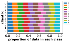
Data heterogeneity: We use a Dirichlet distribution to sample client datasets with different label distributions Hsu and Brown. (2019), and use a tunable parameter () to adjust the amount of data heterogeneity: as shown in Figure 10, the smaller is, the more biased these label distributions will be and the amount of data heterogeneity is higher. When is very small, each client only has data samples of few classes.


Device heterogeneity: To intertwine device heterogeneity with data heterogeneity, we select one data class to be affected by staleness, and apply different amounts of staleness, measured by the number of epochs that clients’ model updates are delayed, to the top 10 clients whose local datasets contain the most data samples of the selected data class. The impact of staleness can be further enlarged by applying staleness in the similar way to more data classes.
We evaluate the FL performance by assessing the trained model’s accuracy in the selected data class being affected by staleness, and evaluate the FL training time in number of epochs. We expect that our approach can either improve the model accuracy, or achieve the similar accuracy with the baselines but use fewer training epochs.
4.2 FL Performance in the Fixed Data Scenario
In the fixed data scenario, 3 standard datasets and 1 domain-specific dataset are used in evaluations:
| Accuracy(%) | MNIST | FMNIST | CIFAR10 | MDI |
| Unweighted | 57.4 | 49.2 | 22.8 | 72.3 |
| Weighted | 39.2 | 30.1 | 12.6 | 61.2 |
| 1st-Order | 57.4 | 49.3 | 22.6 | 72.3 |
| W-Pred | 57.3 | 48.9 | 22.9 | 72.2 |
| Asyn-Tiers | 57.6 | 50.3 | 25.9 | 69.8 |
| Ours | 61.2 | 55.4 | 29.4 | 75.4 |
The trained model’s accuracies444Compared to centralized training, FL models often exhibit lower accuracy, particularly under high data and device heterogeneity, as also reported in existing studies Morafah et al. (2024). using different FL schemes, with the amount of staleness as 40 epochs, are listed in Table 9. The training progresses of 1st-Order and W-Pred closely resemble that of Unweighted aggregation, suggesting that estimating stale model updates with the Taylor expansion is ineffective under unlimited staleness. Similarly, Weighted aggregation will lead to a biased model with much lower accuracy. In contrast, our gradient inversion based compensation can improve the trained model’s accuracy by at least 4%, compared to the best baseline. Such advantage in model accuracy can be as large as 25% when compared with Weighted aggregation. Besides image data, our method is also applicable to other data modalities such as text and time-series data. Results and discussions on these modalities with large real-world datasets are in Appendix A.

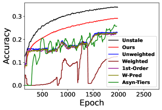
Figure 11 further show the FL training procedure over different epochs, and demonstrated that our method can also improve the progress and stability of training while also achieve higher model accuracy during different stages of FL training. Furthermore, we conducted experiments with different amounts of data and device heterogeneity. Results in Tables 10 and 11 show that555Training times in Tables 10-13 represent the relative training time required to reach convergence of the global model, assuming our method’s training time is 100%., compared with the baselines, our method can generally achieve higher model accuracy or reach the same accuracy with fewer training epochs, especially when the amount of staleness is large or the amount of data heterogeneity is high. We also use other large-scale real-world dataset to conduct experiments and results are in Appendix C.
| 1 | 0.1 | 0.01 | ||||
| Acc | Time | Acc | Time | Acc | Time | |
| Unweighted | 82.3 | 100 | 57.4 | 128 | 51.1 | 132 |
| Weighted | 82.4 | 102 | 39.2 | 171 | 31.1 | 179 |
| 1st-Order | 82.5 | 100 | 57.3 | 129 | 51.5 | 131 |
| W-Pred | 82.8 | 100 | 57.6 | 126 | 50.9 | 131 |
| Asyn-tiers | 82.3 | 97 | 57.6 | 126 | 52.7 | 135 |
| Ours | 82.3 | 100 | 61.2 | 100 | 58.3 | 100 |
| Staleness | 10 | 40 | 100 | |||
| Acc | Time | Acc | Time | Acc | Time | |
| Unweighted | 72.6 | 104 | 57.4 | 128 | 41.5 | 142 |
| Weighted | 69.4 | 115 | 39.2 | 171 | 30.5 | 179 |
| 1st-Order | 72.6 | 104 | 57.3 | 129 | 41.8 | 141 |
| W-Pred | 72.6 | 104 | 57.6 | 126 | 41.7 | 142 |
| Asyn-tiers | 72.7 | 103 | 57.6 | 126 | 38.3 | 138 |
| Ours | 73.3 | 100 | 61.2 | 100 | 47.2 | 100 |
4.3 FL Performance in the Variant Data Scenario

To continuously vary the global data distributions, we use two public datasets, namely MNIST and SVHN Netzer (2011), which are for the same learning task but with different feature representations as shown in Figure 12. Each client’s local dataset is initialized as the MNIST dataset in the same way as in the fixed data scenario. Afterwards, during training, each client continuously replaces random data samples in its local dataset with new data samples in the SVHN dataset.

Experiment results in Figure 13 show that in such variant data scenario, since clients’ local data distributions continuously change, the FL training will never converge. Hence, the model accuracy achieved by the existing FL schemes exhibited significant fluctuations over time and stayed low (40%). In comparison, our technique can better depict the variant data patterns and hence achieve much higher model accuracy, which is comparable to FL without staleness and 20% higher than those in existing FL schemes.
| Staleness | 10 | 40 | 100 | |||
| Acc | Time | Acc | Time | Acc | Time | |
| Unweighted | 60.6 | 99 | 53.2 | 117 | 39.1 | 131 |
| Weighted | 59.8 | 109 | 38.9 | 153 | 21.8 | 166 |
| 1st-Order | 60.6 | 100 | 53.6 | 117 | 40.0 | 133 |
| W-Pred | 60.4 | 100 | 53.3 | 117 | 39.1 | 131 |
| Asyn-tiers | 58.2 | 103 | 46.9 | 118 | 35.7 | 137 |
| Ours | 63.3 | 100 | 62.5 | 100 | 61.0 | 100 |
We also conducted experiments with different amounts of staleness and different rates of data distributions’ variations. We apply different variation rates of clients’ local data distributions by replacing different amounts of such random data samples in the clients’ local datasets in each epoch. To prevent the training from stopping too early when the variation rate is high, we repeatedly varied the data when the variation rate exceeded 1 sample per epoch. Results in Tables 12 and 13 showed that our method outperformed the baselines with different amounts of staleness. Weighted aggregation performs the worst since it leads the model to bias toward other unstable clients and other baselines show similar performance since they cannot compensate such large staleness.
| Rate | 0.5 | 1 | 2 | |||
| Acc | Time | Acc | Time | Acc | Time | |
| Unweighted | 73.1 | 100 | 39.1 | 131 | 44.1 | 127 |
| Weighted | 58.2 | 102 | 21.8 | 166 | 25.2 | 163 |
| 1st-Order | 73.2 | 100 | 40.0 | 133 | 43.9 | 127 |
| W-Pred | 73.1 | 101 | 39.0 | 131 | 39.5 | 127 |
| Asyn-tiers | 68.3 | 98 | 35.7 | 137 | 39.1 | 130 |
| Ours | 70.3 | 100 | 60.1 | 100 | 63.3 | 100 |
5 Related Work
Most existing solutions to staleness in FL are based on weighted aggregation Chen and Jin. (2019); Wang (2022); Chen (2020). These existing solutions are biased towards fast clients, and will affect the trained model’s accuracy when data and device heterogeneities in FL are intertwined. Other researchers suggest to use semi-asynchronous FL, where the server aggregates client model updates at a lower frequency Nguyen (2022) or clusters clients into different asynchronous “tiers” according to their update rates Chai (2021). However, doing so cannot completely eliminate the impact of intertwined data and device heterogeneities, because the server’s aggregation still involves stale model updates.
Instead, we can transfer knowledge from stale model updates to the global model, by training a generative model and compelling its generated data to exhibit high predictive values on the original model updates Ye (2020); Lopes et al. (2017); Zhu et al. (2021). Another approach is to optimize randomly initialized input data until it has good performance on the original model YYin (2020). However, the quality and accuracy of knowledge transfer in these methods remains low, and we provided more detailed experiment results in Appendix C to demonstrate such low quality. Other efforts enhance the quality of knowledge transfer by incorporating natural image priors Luo (2020) or using another public dataset to introduce general knowledge Yang (2019), but require extra datasets. Moreover, all these methods require that the clients’ local models to be fully trained, which is usually infeasible in FL.
6 Conclusion
In this paper, we present a new FL framework to tackle intertwined data and device heterogeneities in FL, by using gradient inversion to estimate clients’ unstale model updates. Experiments show that our technique largely improves model accuracy and reduces the amount of training epochs needed.
Acknowledgments
We thank the anonymous reviewers for their comments and feedback. This work was supported in part by National Science Foundation (NSF) under grant number IIS-2205360, CCF-2217003, CCF-2215042, and National Institutes of Health (NIH) under grant number R01HL170368.
References
- Ahmed et al. [2020] L. Ahmed, K. Ahmad, N. Said, B. Qolomany, J. Qadir, and A. Al-Fuqaha. Active learning based federated learning for waste and natural disaster image classification. IEEE Access, 8:208518–208531, 2020.
- Chai [2021] e. a. Chai, Zheng. FedAT: A high-performance and communication-efficient federated learning system with asynchronous tiers. In Proceedings of the International Conference for High Performance Computing, Networking, Storage and Analysis, 2021.
- Chai et al. [2021] Z. Chai, Y. Chen, A. Anwar, L. Zhao, Y. Cheng, and H. Rangwala. Fedat: A high-performance and communication-efficient federated learning system with asynchronous tiers. In Proceedings of the International Conference for High Performance Computing, Networking, Storage and Analysis, pages 1–16, 2021.
- Charles et al. [2021] Z. Charles, Z. Garrett, Z. Huo, S. Shmulyian, and V. Smith. On large-cohort training for federated learning. Advances in neural information processing systems, 34:20461–20475, 2021.
- Charpiat [2019] e. a. Charpiat, Guillaume. Input similarity from the neural network perspective. In Advances in Neural Information Processing Systems 32, 2019.
- Chen [2020] e. a. Chen, Yujing. Asynchronous online federated learning for edge devices with non-iid data. In 2020 IEEE International Conference on Big Data (Big Data), 2020.
- Chen and Jin. [2019] X. S. Chen, Yang and Y. Jin. Communication-efficient federated deep learning with layerwise asynchronous model update and temporally weighted aggregation. In IEEE transactions on neural networks and learning systems, 2019.
- Chen et al. [2017] Y. Chen, X. Yang, B. Chen, C. Miao, and H. Yu. Pdassist: Objective and quantified symptom assessment of parkinson’s disease via smartphone. In 2017 IEEE International Conference on Bioinformatics and Biomedicine (BIBM), pages 939–945. IEEE, 2017.
- Dimitrov et al. [2022] D. I. Dimitrov, M. Balunović, N. Jovanović, and M. Vechev. Lamp: Extracting text from gradients with language model priors. arXiv e-prints, pages arXiv–2202, 2022.
- Geiping [2020] e. a. Geiping, Jonas. Inverting gradients-how easy is it to break privacy in federated learning? In Advances in Neural Information Processing Systems 33, 2020.
- Geyer et al. [2017] R. C. Geyer, T. Klein, and M. Nabi. Differentially private federated learning: A client level perspective. arXiv preprint arXiv:1712.07557, 2017.
- Gupta et al. [2022] S. Gupta, Y. Huang, Z. Zhong, T. Gao, K. Li, and D. Chen. Recovering private text in federated learning of language models. Advances in neural information processing systems, 35:8130–8143, 2022.
- Hakimi et al. [2019] I. Hakimi, S. Barkai, M. Gabel, and A. Schuster. Taming momentum in a distributed asynchronous environment. arXiv preprint arXiv:1907.11612, 2019.
- Heusel et al. [2017] M. Heusel, H. Ramsauer, T. Unterthiner, B. Nessler, and S. Hochreiter. Gans trained by a two time-scale update rule converge to a local nash equilibrium. Advances in neural information processing systems, 30, 2017.
- Hsu and Brown. [2019] H. Q. Hsu, Tzu-Ming Harry and M. Brown. Measuring the effects of non-identical data distribution for federated visual classification. In arXiv preprint, 2019.
- Karimireddy [2020] e. a. Karimireddy, Sai Praneeth. Scaffold: Stochastic controlled averaging for federated learning. In International conference on machine learning. PMLR, 2020.
- Konečný [2016] e. a. Konečný, Jakub. Federated optimization: Distributed machine learning for on-device intelligence. In arXiv preprint arXiv:1610.02527, 2016.
- Krizhevsky [2009] a. G. H. Krizhevsky, Alex. Learning multiple layers of features from tiny images. 2009.
- LeCun and Burges. [2010] C. C. LeCun, Yann and C. Burges. Mnist handwritten digit database. http://yann.lecun.com/exdb/mnist, 2010.
- Li et al. [2020] T. Li, A. K. Sahu, M. Zaheer, M. Sanjabi, A. Talwalkar, and V. Smith. Federated optimization in heterogeneous networks. Proceedings of Machine learning and systems, 2:429–450, 2020.
- Li et al. [2023a] X. Li, Z. Qu, B. Tang, and Z. Lu. Fedlga: Toward system-heterogeneity of federated learning via local gradient approximation. IEEE Transactions on Cybernetics, 54(1):401–414, 2023a.
- Li et al. [2023b] Z. Li, T. Lin, X. Shang, and C. Wu. Revisiting weighted aggregation in federated learning with neural networks. arXiv preprint arXiv:2302.10911, 2023b.
- Lin et al. [2017] Y. Lin, S. Han, H. Mao, Y. Wang, and W. J. Dally. Deep gradient compression: Reducing the communication bandwidth for distributed training. arXiv preprint arXiv:1712.01887, 2017.
- Lopes et al. [2017] R. G. Lopes, S. Fenu, and T. Starner. Data-free knowledge distillation for deep neural networks. arXiv preprint arXiv:1710.07535, 2017.
- Luo [2020] e. a. Luo, Liangchen. Large-scale generative data-free distillation. In arXiv preprint arXiv:2012.05578, 2020.
- McMahan [2016] e. a. McMahan, Brendan. Communication-efficient learning of deep networks from decentralized data. In arXiv preprint, 2016.
- Morafah et al. [2024] M. Morafah, V. Kungurtsev, H. Chang, C. Chen, and B. Lin. Towards diverse device heterogeneous federated learning via task arithmetic knowledge integration. arXiv preprint arXiv:2409.18461, 2024.
- Mouzannar et al. [2018] H. Mouzannar, Y. Rizk, and M. Awad. Damage identification in social media posts using multimodal deep learning. In ISCRAM. Rochester, NY, USA, 2018.
- Netzer [2011] e. a. Netzer, Yuval. Reading digits in natural images with unsupervised feature learning. In Advances in Neural Information Processing Systems 32, 2011.
- Nguyen [2022] e. a. Nguyen, John. Federated learning with buffered asynchronous aggregation. In International Conference on Artificial Intelligence and Statistics. PMLR, 2022.
- Reddi et al. [2020] S. Reddi, Z. Charles, M. Zaheer, Z. Garrett, K. Rush, J. Konečnỳ, S. Kumar, and H. B. McMahan. Adaptive federated optimization. arXiv preprint arXiv:2003.00295, 2020.
- Reiss and Stricker [2012] A. Reiss and D. Stricker. Introducing a new benchmarked dataset for activity monitoring. In 2012 16th international symposium on wearable computers, pages 108–109. IEEE, 2012.
- Ro et al. [2022] J. H. Ro, T. Breiner, L. McConnaughey, M. Chen, A. T. Suresh, S. Kumar, and R. Mathews. Scaling language model size in cross-device federated learning. arXiv preprint arXiv:2204.09715, 2022.
- Shi et al. [2020] G. Shi, L. Li, J. Wang, W. Chen, K. Ye, and C. Xu. Hysync: Hybrid federated learning with effective synchronization. In 2020 IEEE 22nd International Conference on High Performance Computing and Communications; IEEE 18th International Conference on Smart City; IEEE 6th International Conference on Data Science and Systems (HPCC/SmartCity/DSS), pages 628–633. IEEE, 2020.
- Tian et al. [2021] P. Tian, Z. Chen, W. Yu, and W. Liao. Towards asynchronous federated learning based threat detection: A dc-adam approach. Computers & Security, 108:102344, 2021.
- Vaizman et al. [2017] Y. Vaizman, K. Ellis, and G. Lanckriet. Recognizing detailed human context in the wild from smartphones and smartwatches. IEEE pervasive computing, 16(4):62–74, 2017.
- Wang [2022] e. a. Wang, Qiyuan. AsyncFedED: Asynchronous Federated Learning with Euclidean Distance based Adaptive Weight Aggregation. In arXiv preprint, 2022.
- Wang et al. [2021] J. Wang, Z. Charles, Z. Xu, G. Joshi, H. B. McMahan, M. Al-Shedivat, G. Andrew, S. Avestimehr, K. Daly, D. Data, et al. A field guide to federated optimization. arXiv preprint arXiv:2107.06917, 2021.
- Wang et al. [2020] Y. Wang, T. Zhu, W. Chang, S. Shen, and W. Ren. Model poisoning defense on federated learning: A validation based approach. In International Conference on Network and System Security, pages 207–223. Springer, 2020.
- Wu et al. [2023] Y. Wu, S. Zhang, W. Yu, Y. Liu, Q. Gu, D. Zhou, H. Chen, and W. Cheng. Personalized federated learning under mixture of distributions. In International Conference on Machine Learning, pages 37860–37879. PMLR, 2023.
- Xiao et al. [2017] H. Xiao, K. Rasul, and R. Vollgraf. Fashion-mnist: a novel image dataset for benchmarking machine learning algorithms. arXiv preprint arXiv:1708.07747, 2017.
- Xie and Gupta. [2019] S. K. Xie, Cong and I. Gupta. Asynchronous federated optimization. In arXiv preprint, 2019.
- Yang [2019] e. a. Yang, Ziqi. Neural network inversion in adversarial setting via background knowledge alignment. In Proceedings of the 2019 ACM SIGSAC Conference on Computer and Communications Security., 2019.
- Ye [2020] e. a. Ye, Jingwen. Data-free knowledge amalgamation via group-stack dual-gan. In Proceedings of the IEEE/CVF Conference on Computer Vision and Pattern Recognition, 2020.
- Yin [2020] e. a. Yin, Hongxu. Dreaming to distill: Data-free knowledge transfer via deepinversion. In Proceedings of the IEEE/CVF Conference on Computer Vision and Pattern Recognition, 2020.
- Yin [2021] e. a. Yin, Hongxu. See through gradients: Image batch recovery via gradinversion. In Proceedings of the IEEE/CVF Conference on Computer Vision and Pattern Recognition, 2021.
- YYin [2020] e. a. YYin, Hongxu. Dreaming to distill: Data-free knowledge transfer via deepinversion. In Proceedings of the IEEE/CVF Conference on Computer Vision and Pattern Recognition., 2020.
- Zhang [2018] e. a. Zhang, Richard. The unreasonable effectiveness of deep features as a perceptual metric. In Proceedings of the IEEE conference on computer vision and pattern recognition, 2018.
- Zhao [2018] e. a. Zhao, Yue. Federated learning with non-iid data. In arXiv preprint, 2018.
- Zhao and Bilen. [2020] K. R. M. Zhao, Bo and H. Bilen. idlg: Improved deep leakage from gradients. In arXiv preprint arXiv:2001.02610, 2020.
- Zheng et al. [2017] S. Zheng, Q. Meng, T. Wang, W. Chen, N. Yu, Z.-M. Ma, and T.-Y. Liu. Asynchronous stochastic gradient descent with delay compensation. In International Conference on Machine Learning, pages 4120–4129. PMLR, 2017.
- Zhou [2021] e. a. Zhou, Chendi. TEA-fed: time-efficient asynchronous federated learning for edge computing. In Proceedings of the 18th ACM International Conference on Computing Frontiers, 2021.
- Zhou and Lv. [2021] Q. Y. Zhou, Yuhao and J. Lv. Communication-efficient federated learning with compensated overlap-fedavg. In IEEE Transactions on Parallel and Distributed Systems, 2021.
- Zhou et al. [2021] Y. Zhou, Q. Ye, and J. Lv. Communication-efficient federated learning with compensated overlap-fedavg. IEEE Transactions on Parallel and Distributed Systems, 33(1):192–205, 2021.
- Zhu et al. [2022] H. Zhu, J. Kuang, M. Yang, and H. Qian. Client selection with staleness compensation in asynchronous federated learning. IEEE Transactions on Vehicular Technology, 72(3):4124–4129, 2022.
- Zhu et al. [2019] L. Zhu, Z. Liu, and S. Han. Deep leakage from gradients. Advances in neural information processing systems, 32, 2019.
- Zhu et al. [2021] Z. Zhu, J. Hong, and J. Zhou. Data-free knowledge distillation for heterogeneous federated learning. In International conference on machine learning, pages 12878–12889. PMLR, 2021.
- Zhu and Han. [2019a] Z. L. Zhu, Ligeng and S. Han. Deep leakage from gradients. In Advances in neural information processing systems, 2019a.
- Zhu and Han. [2019b] Z. L. Zhu, Ligeng and S. Han. Deep leakage from gradients. In Advances in neural information processing systems 32, 2019b.
Appendix A A: Evaluations with other data modalities
In the experimental section of the main text, we conduct experiments on three benchmark CV datasets and one real-world CV dataset. To demonstrate the generality of our method, we further conduct experiments on two human activity recognition (HAR) datasets with time-series data:
-
•
PAMAP2 Reiss and Stricker [2012] with 13 classes of human activities and over 2M data samples collected using IMU and heart rate sensors. A 3-layer MLP model is used in FL.
-
•
ExtraSensory Vaizman et al. [2017] with over 300k data samples collected using IMU, gyroscope and magnetometer sensors on smartphones. Besides 7 main labels of activities (e.g., standing, laying down, etc), it also provides 109 additional labels describing more specific activity contexts. An 1D-CNN model is used in FL.
We set three levels of staleness to 2, 5, and 10 epochs, while other settings remain the same as those in the main results. As shown in Table 14, our approach demonstrates an advantage under medium or high staleness.
| PAMAP2 / MLP | ExtraSensory / 1D-CNN | |||||
| staleness | low | medium | high | low | medium | high |
| Unweighted | 0.0% | 0.0% | 0.0% | 0.0% | 0.0% | 0.0% |
| Weighted | -5.4% | -13.9% | -43.5% | -18.4% | -46.5% | -62.3% |
| Asyn-tiers | +0.7% | +0.4% | -0.5% | -2.0% | +0.8% | -2.9% |
| 1st-Order | +2.3% | +1.5% | +0.6% | +3.6% | +2.5% | -2.2% |
| W-Pred | +2.6% | +1.3% | +0.6% | +0.4% | +1.5% | -1.3% |
| Ours | -1.9% | +5.4% | 70.6% | -3.0% | +16.9% | +34.2% |
Besides, our method can also be applied to tasks involving other data modalities, such as text. Since in NLP, text is decomposed into discrete tokens, we must estimate data in the continuous embedding space Zhu et al. [2019]. Since errors occur when projecting the estimated data from the embedding space into discrete tokens, text is more prone to gradient inversion attacks, requiring prior knowledge for a successful attack Gupta et al. [2022], Dimitrov et al. [2022]. This suggests that when applied to test data, the privacy leakage risk of our method would be lower.
Appendix B B: Comprehensive evaluation on weighted aggregation
Applying a smaller weight to a stale update can reduce the error introduced in Federated training. However, under intertwined heterogeneities, applying reduced weights to stale updates degrades the accuracy of data samples affected by these heterogeneities. This occurs because the contributions of these data to the global model are also reduced, so the trained global model contains less knowledge about these data.
Intuitively, if we increase the weight of stale updates, their contributions are forced to increase, leading to higher accuracy on the stale clients. However, the errors in the stale updates are also magnified and incorporated into the global model, which decreases the model’s accuracy on other data. To verify this, we simulate an FL system with 100 clients, 10 of which are stale, and train a LeNet model on the MNIST dataset. As shown in Table 15, compared to unweighted updates, applying increased weight improves the accuracy on the 10 stale clients by around 10%, but decreases the overall accuracy across all 100 clients by around 5%. Clearly, such a trade-off is unacceptable. Therefore, we should compensate the error in the stale updates instead of exploring weighting strategies.
| Weighting strategy | Reduced W | Non | Increased W |
| Acc - stale clients (%) | 39.2 | 57.4 | 68.1 |
| Acc - all clients (%) | 81.4 | 80.5 | 75.4 |
| Method | GI based estimation | direct aggregation | using samples from generative model |
| Estimation error | 0.32 | 0.52 | 0.86 |
Appendix C C: Other approaches to estimating the data knowledge
Our basic approach in this paper is to use the gradient inversion technique Zhu and Han. [2019a], Zhao and Bilen. [2020] to estimate knowledge about the clients’ local training data from their uploaded stale model updates, and then use such estimated knowledge to compute the corresponding non-stale model updates for aggregation in FL. In this section, we provide supplementary justifications about the ineffectiveness of other methods for such data knowledge estimation, hence better motivating our proposed design.

The most commonly used approach to recovering the training data from a trained ML model involves training an extra generative model, to compel its generated data samples to exhibit high predictive value on the original model Zhu et al. [2021], and to add image prior constraint terms to enhance data quality Luo [2020]. On the other hand, data recovery can also be achieved by directly optimizing randomly initialized input data until it performs well on the original model YYin [2020]. However, the results of our preliminary experiments, using the LeNet model and and the MNIST dataset, show that none of these approaches can provide good quality of the computed data, in order to be used in our FL scenarios.
More specifically, these existing approaches can ensure that the computed dataset, as a whole, exhibits some characteristics of the original training data. For example, as shown in Figure 14, the averaged image of the recovered data samples in each data class can resemble a meaningful image that matches the data pattern in the original dataset. However, the individual image samples being computed have very low quality. If these computed data samples are used to compute the non-stale model updates in FL, it will result in a significant error in estimating the non-stale model updates, which greatly exceeds the error produced by our proposed gradient inversion (GI) based estimation, as shown in Table 16.

Furthermore, as shown in Figure 15, the computed data samples lack diversity, resulting in high similarity among the generated samples in the same data class. Training on such highly similar data samples can easily lead the model to overfit.

Some attempts have been made to enhance the data quality by incorporating another extra public dataset to introduce general image knowledge Yang [2019], but the effectiveness of this approach highly depends on the specific choice of such public dataset. Experimental results in jeon2021gradient demonstrate that the quality of computed data can only be ensured if the extra public dataset shares the similar data pattern with the original training dataset. For example, in our preliminary experiments, we selected CIFAR-100 as the public dataset, and the original training datasets included CIFAR-10 and SVHN datasets. As shown in Figure 16, when CIFAR-10 is used as the training dataset, the computed data exhibits higher quality compared with that using the SVHN dataset as the training dataset, because the CIFAR-10 dataset shares the similar image patterns with the CIFAR-100 dataset.
Compared to the existing methods, our proposed technique uses gradient inversion to obtain an estimation of the clients’ original training data. Since we only require the computed data to mimic the model’s gradient produced with the original training data, we do not necessitate the quality of individual data samples being computed, and could hence avoid the impact of the computed data’s low quality on the FL performance.

.
Because of such low quality of the computed data, they cannot be directly used to retrain the global model in FL, as an estimate to non-stale model updates. Some existing approaches, instead, use knowledge distillation to transfer the knowledge contained in the computed data to the target ML model Zhu et al. [2021]. However, in our FL scenario, since the server only conducts aggregation of the received clients’ model updates and lacks the corresponding test data (as part of the clients’ local data), the server will be unable to decide if and when the model retraining will overfit (Figure 17). Furthermore, all the existing methods require that the clients’ model updates have to be fully trained, but this requirement generally cannot be satisfied in FL scenarios.
Appendix D D: Hyper-parameters in gradient inversion
Deciding the size of : In our proposed approach to estimating the clients’ local data distributions from stale model updates, a key issue is how to decide the proper size of . Since gradient inversion is equivalent to data resampling in the original training data’s distribution, a sufficiently large size of would be necessary to ensure unbiased data sampling and sufficient minimization of gradient loss through iterations. On the other hand, when the size of is too large, the computational overhead of each iteration would be unnecessarily too high.
We experimentally investigated such tradeoff by using the MNIST and CIFAR-10 Krizhevsky [2009] datasets to train a LeNet model. Results in Tables 17 and 18, where the size of is represented by its ratio to the size of original training data, show that when the size of is larger than 1/2 of the size of the original training data, further increasing the size of only results in little extra reduction of the gradient inversion loss but dramatically increase the computational overhead. Hence, we believe that it is a suitable size of for FL. Considering that clients’ local dataset in FL contain at least hundreds of samples, we expect a big size of in most FL scenarios.
| Size | 1/64 | 1/16 | 1/4 | 1/2 | 2 | 10 |
| Time(s) | 193 | 207 | 214 | 219 | 564 | 2097 |
| GI loss | 27 | 4.1 | 2.56 | 1.74 | 1.62 | 1.47 |
| Size | 1/64 | 1/16 | 1/4 | 1/2 | 2 | 10 |
| Time(s) | 423 | 440 | 452 | 474 | 1330 | 4637 |
| GI Loss | 1.97 | 0.29 | 0.16 | 0.15 | 0.15 | 0.12 |
Deciding the metric for model difference: Such a big size of directly decides our choice of how to evaluate the change of in Eq. (2). Most existing works use cosine similarity between and to evaluate their difference in the direction of gradients, so as to maximize the quality of individual data samples in Charpiat [2019]. However, since we aim to compute a large , this metric is not applicable, and instead we use L1-norm as the metric to evaluate how using to retrain will change its magnitude of gradient, to make sure that incurs the minimum impact on the state of training.
Appendix E E: Gradient inversion under diverse FL settings
In the main text of the paper, we empirically verified that our gradient inversion-based compensation achieves significantly smaller error compared to first-order compensation in a simple FL setting. However, in FL, many factors can affect the training process. Therefore, in this section, we further evaluate the error under diverse settings to demonstrate that our methods have broad applications in real-world FL systems.
The first factor we consider is the number of steps in local training, as existing works Geiping [2020] indicate that a complex local training program makes gradient inversion more difficult. Under such a high degree of data heterogeneity, the divergence between the client model and the global model increases with the number of local stepsKarimireddy [2020], making compensation more challenging. We use the LeNet model, the MNIST dataset, and an SGD optimizer to compute a stale update and apply different methods to compensate for it. The results are shown in Table 19. Although the error of our method increases with the number of steps, it remains much smaller than that of the first-order method.
| # of iterations | 1 | 5 | 10 | 20 | 50 |
| GI method | 0.05 | 0.18 | 0.22 | 0.22 | 0.26 |
| 1st-order method | 0.14 | 0.31 | 0.33 | 0.35 | 0.38 |
Except for basic SGD, various optimizers are used in different FL systems. We test our methods with four optimizers: SGD, SGD with momentum (SGDM), Adam, and FedProx, where FedProx is an optimization method designed for FL with data heterogeneity by using a proximal term Li et al. [2020]. As shown in Table 20, our method can achieve a smaller compensation error with most optimizers. Although our method fails when using adaptive optimizers like Adam, in our practice, under a high degree of data heterogeneity, it’s not recommended to use these adaptive optimizers for training stability.
| Optimizer | SGD | SGDM | Adam | FedProx |
| GI method | 0.22 | 0.26 | 0.44 | 0.17 |
| 1st-order method | 0.33 | 0.35 | 0.38 | 0.30 |
Appendix F F: Error caused by gradient sparsification
In the main text of the paper, we showed that with 95% sparsification, we can reduce computation and protect privacy with only a small increase in estimation error. To better evaluate the trade-off between performance and efficiency/privacy, we further compare the training accuracy at different rates of sparsification using LeNet and MNIST dataset. As shown in Table 21, with a sparsification rate of 95%, the accuracy drop compared to non-sparsification is minor, but is high enough to achieve computation savings and privacy protection. Further increase the sparsification rate will help reduce more computation in the gradient inversion, but the accuracy drop is significant.
| Sparsification rate | 0% | 90% | 95% | 99% |
| Accuracy | 63.5 | 61.9 | 61.2 | 53.3 |
Appendix G G: Other Discussions
G.1 Server’s overhead in large-scale FL systems
In large-scale FL systems, the server must compute gradients for each delayed client, potentially leading to a performance bottleneck. However, our method requires applying gradient inversion only to a subset of stale model updates, which encapsulate unique and critical knowledge absent from other unstable updates. We argue that, in most practical scenarios as we listed in the main text of the paper, the volume of these updates is likely to remain small, even in large-scale FL systems.
On the other hand, most of current FL implementations, such as Charles et al. [2021], usually use a variant client selection rate, so that the number of clients participating in one global round remains constant instead of increasing proportionally with the total number of clients. Essentially, existing work Ro et al. [2022] showed that once the number of clients per global round is sufficiently large (e.g., 10-50 even for FL systems with thousands of clients), further increasing such number yields only marginal performance gains but significantly increases overhead, and could also result in catastrophic training failure and generalization failure. Hence, our approach will not significantly increase the server’s computing overhead in large-scale FL systems.
G.2 Defense against malicious attackers
In practical FL systems, a malicious attacker may intentionally inject abrupt gradients (e.g., with extremely large or small values) into the server. Such attacks not only disrupt gradient inversion but also undermine the FL training process itself, hindering convergence and reducing model accuracy. While defending against such attacks is not the primary focus of this paper, existing works have proposed defenses against these gradient-based attacks Wang et al. [2020].
G.3 Applying statistical privacy methods
Since our method only modifies the FL operations on the server and keeps other FL steps (e.g., the clients’ local model updates and client-server communication) unchanged, local differential privacy can theoretically be directly applied to our approach without any modification. More specifically, each client can independently add Gaussian noise to its local model updates, before sending the updates to the server Geyer et al. [2017].
Moreover, note that differential privacy (DP) is also orthogonal to our proposed privacy protection method, because noise can be added to the gradient after our proposed sparsification method.