This paper was converted on www.awesomepapers.org from LaTeX by an anonymous user.
Want to know more? Visit the Converter page.

T-odd generalized and quasi transverse momentum dependent parton distribution in a scalar spectator model

Xuan Luo    Hao Sun111Corresponding author: [email protected]    [email protected] Institute of Theoretical Physics, School of Physics, Dalian University of Technology,
No.2 Linggong Road, Dalian, Liaoning, 116024, P.R.China
Abstract

Generalized transverse momentum dependent parton distributions (GTMDs), as mother funtions of transverse momentum dependent parton distributions (TMDs) and generalized parton distributions (GPDs), encode the most general parton structure of hadrons. We calculate four twist-two time reversal odd GTMDs of pion in a scalar spectator model. We study the dependence of GTMDs on the longitudinal momentum fraction xx carried by the active quark and the transverse momentum |kT||\vec{k}_{T}| for different values of skewness ξ\xi defined as the longitudinal momentum transferred to the proton as well as the total momentum |ΔT||\vec{\Delta}_{T}| transferred to the proton. In addition, the quasi-TMDs and quasi-GPDs of pion have also been investigated in this paper.

I INTRODUCTION

Exploring the partonic substructure of hadrons is still at the frontier of hadronic high energy physics research. The parton distribution functions (PDFs) make it clear how the longitudinal parton momentums in hadron are distributed. However, they only include one dimension information. Therefore probing how partons distribute in the transverse plane in both momentum and coordinate space becomes a vital topic. Typically, the transverse spatial distribution of partons inside a hadron can be quantified by Generalised parton distributions (GPDs) Diehl (2003); Belitsky and Radyushkin (2005); Garcon (2002), which can be denoted as a function of longitudinal momentum fraction xx carried by the parton, the longitudinal momentum ξ\xi transferred to the hadron and the total momentum transferred tt. They can be accessed through measurements in hard exclusive reactions like deep virtual Compton scattering and hard exclusive meson production Goeke et al. (2001); Belitsky and Radyushkin (2005). While the transverse momentum dependent parton distributions (TMDs) Collins and Soper (1982); Bacchetta et al. (2007); Meissner et al. (2007) depending on both the longitudinal and transverse motion of partons inside a hadron can be studied by the description of various hard semi-inclusive reactions. More general distibutions than the GPDs and the TMDs, the generalized transverse momentum dependent parton distributions (GTMDs) Meissner et al. (2008, 2009); Lorcé and Pasquini (2013) could reduce to them in specific kinematical limits, therefore serve as mother distributions. The GTMDs can directly enter the description of hard exclusive reactions. The parametrization of the generalized quark-quark correlation functions for a spin-0 and spin-1/21/2 hadron in terms of GTMDs are given in Refs.Meissner et al. (2008, 2009). Then the authors in Ref.Lorcé and Pasquini (2013) add a complete classification of gluon GTMDs. Particularly, the correlator related to the time-reversal odd (T-odd) GTMDs is contributed by the final state interactions from gauge link or Wilson line. These interactions are necessary to generate the single spin asymmetries Brodsky et al. (2002).

Although PDFs are related to parton fields in QCD, it is difficult to calculate them directly in QCD since they are nonperturbative quantities. This difficulties may be overcomed by Lattice QCD method studying the PDFs from first principles. However, PDFs are usually defined on the light cone, which poses a problem for the standard Euclidean formulation, and in lattice QCD calculation only moments of distributions in xx can be accessed as matrix elements of local operators Dolgov et al. (2002); Gockeler et al. (2005). To overcome these issues, the proposed large-momentum effective theory (LaMET) of Ji has been presented Ji (2013). This method evaluates PDFs on the lattice through quasi-PDFs Ji (2013); Ma and Qiu (2018); Ji (2014), whose mother correlation functions includes a spacelike operator γz\gamma^{z} instead of the usual lightlike γ+\gamma^{+} entering the definition of the standard PDFs. These quasi-PDFs can be reached directly from the lattice QCD calculation Lin et al. (2015) and as the quasi-PDFs depend logarithmically on PzP_{z} when PzP_{z} becomes large, and they need a perturbative matching in LaMET to reduce to the standard PDFs. A very recent review of LaMET is given in Ji et al. (2020). Many theoretical discussions and lattice simulations for quasi-PDFs and similar quantities has been performed Orginos et al. (2017); Green et al. (2018); Alexandrou et al. (2015); Chen et al. (2016); Alexandrou et al. (2017a); Zhang et al. (2017); Lin et al. (2018a); Bali et al. (2018); Alexandrou et al. (2018a); Zhang et al. (2019a); Alexandrou et al. (2018b); Chen et al. (2018a); Zhang et al. (2019b); Alexandrou et al. (2018c); Liu et al. (2020); Lin et al. (2018b). Moreover, several model calculations of quasi-PDFs have been carried out Gamberg et al. (2015); Bacchetta et al. (2017); Nam (2017); Broniowski and Ruiz Arriola (2017); Hobbs (2018); Broniowski and Ruiz Arriola (2018); Xu et al. (2018). There have also been a number of works on quasi-PDFs renormalization Chen et al. (2018b); Green et al. (2018); Ji et al. (2018); Ishikawa et al. (2017); Alexandrou et al. (2017b); Constantinou and Panagopoulos (2017); Xiong et al. (2017); Chen et al. (2017); Ishikawa et al. (2016). The approach Ji (2013) can be generalized to any light-cone correlations in hadron physics, e.g. the correlators related to GPDs and TMDs. There has been a lot of efforts on the quasi-TMDs, including their renormalization and matching to the physical TMDs Ji et al. (2015, 2019a); Ebert et al. (2019a, b, 2020a); Ji et al. (2019b, c); Vladimirov and Schäfer (2020); Ji et al. (2020); Ebert et al. (2020b). These quasi-TMD works have made important breakthroughs on their pinched-pole singularity issue, renormalization, evolution, soft factor subtraction, and factorization into physical TMDs. Moreover, the nonperturbative Collins-Soper evolution kernel of TMDs has been calculated in Shanahan et al. (2020a, b) , which is an important step in TMDs full extractions from lattice QCD. In summary, it may be useful to study the quasi-distributions such as quasi-PDFs, quasi-GPDs and quasi-TMDs.

Among the hadrons, pions are very fascinating particles and they hold a lot of information on the structure of hadrons. There has been a tremendous effort to deduce the parton distribution functions of the pion. Pions provide the force that binds the protons and neutrons inside the nuclei and they also influence the properties of the isolated nucleons. Thus understanding of matter is not complete without getting a detailed information on the role of pions. In this paper, being inspired by the previous works for quasi-distribution model calculations Bhattacharya et al. (2019a, b); Ma et al. (2019), we will probe the T-odd GTMDs, quasi-TMDs and the quasi-GPDs of the pion applying a scalar spectator model. In particular, GPDs of the pion have been obtained in various models like chiral quark model Broniowski and Ruiz Arriola (2003); Dorokhov et al. (2011), NJL model Davidson and Ruiz Arriola (2002); Theussl et al. (2004), light-front constituent quark model Frederico et al. (2009) and lattice QCD Brömmel et al. (2008); Sufian et al. (2020); Izubuchi et al. (2019); Chen et al. (2019). We will give out the analytical results of all four twist-two T-odd GTMDs, quasi-TMDs and quasi-GPDs in the present paper, and conduct a qualitative analysis of all these distributions.

The remainder of this paper is as follows: Sec.II below describes in detail the theoretical definition of various pion parton distributions. In Sec.III we give out the analytical results of four T-odd GTMDs, quasi-TMDs and quasi-GPDs in a scalar spectator. In Sec.IV, we present our numerical studies using a group of fitted model parameters of a scalar spectator model. A brief conclusion is presented in Sect.V.

II Definition of pion parton distributions

II.1 Transverse momentum dependent parton distribution h1πh_{1\pi}^{\perp}

For a spinless particle, such as the pion, only two leading twist TMDs arise, in contrast to the eight found for spin-12\frac{1}{2} particles Barone et al. (2010). The TMD f1πf_{1\pi} is simply the unpolarized quark distribution, whereas the Boer-Mulders (BM) function Boer and Mulders (1998), h1πh_{1\pi}^{\perp}, describes the distribution of transversely polarized quarks in the pion. The BM function h1πh_{1\pi}^{\perp} is defined from the quark-quark distribution correlation function

Φ[Γ](x,kT)=12dξd2ξT(2π)3eikξP|ψ¯(12ξ)Γ𝒲+(12ξ;12ξ)ψ(12ξ)|P|ξ+=0,\displaystyle\begin{aligned} \Phi^{[\Gamma]}(x,\vec{k}_{T})=\int\frac{1}{2}\frac{d\xi^{-}d^{2}\vec{\xi}_{T}}{(2\pi)^{3}}e^{ik\cdot\xi}\langle P|\bar{\psi}(-\frac{1}{2}\xi)\Gamma\mathcal{W}_{+\infty}(-\frac{1}{2}\xi;\frac{1}{2}\xi)\psi(\frac{1}{2}\xi)|P\rangle\bigg{|}_{\xi^{+}=0},\end{aligned} (1)

where PP is the four-momentum of the pion moving along the zz-axis with the components (P+,P,0P^{+},P^{-},\vec{0}_{\perp}) in the light-cone coordinates, in which the plus and minus components of any four-vector aμa^{\mu} have the form a±=(a0±a3)/2a^{\pm}=(a^{0}\pm a^{3})/\sqrt{2}, and transverse part a=(a1,a2)\vec{a}_{\perp}=(a^{1},a^{2}). The quark field and momentum are denoted by kk and ψ\psi. In the correlator Eq.(1) we have Wilson lines

𝒲+(12ξ;12ξ)|ξ+=0=[0+,12ξ,12ξT;0+,+,12ξT][0+,+,12ξT;0+,+,12ξT][0+,+,12ξT;0+,12ξ,12ξT],\displaystyle\begin{aligned} \mathcal{W}_{+\infty}(-\frac{1}{2}\xi;\frac{1}{2}\xi)|_{\xi^{+}=0}&=[0^{+},-\frac{1}{2}\xi^{-},-\frac{1}{2}\vec{\xi}_{T};0^{+},+\infty^{-},-\frac{1}{2}\vec{\xi}_{T}]\cdot[0^{+},+\infty^{-},-\frac{1}{2}\vec{\xi}_{T};0^{+},+\infty^{-},\frac{1}{2}\vec{\xi}_{T}]\\ &\cdot[0^{+},+\infty^{-},\frac{1}{2}\vec{\xi}_{T};0^{+},\frac{1}{2}\xi^{-},\frac{1}{2}\vec{\xi}_{T}],\end{aligned} (2)

where

[0+,12ξ,12ξT;0+,+,12ξT]=𝒫exp[igs12ξ+𝑑ζA+(ζ,0+,12ξT)],[0+,+,12ξT;0+,+,12ξT]=𝒫exp[igs12ξT12ξT𝑑ζTAT(+,0+,ζT)],[0+,+,12ξT;0+,12ξ,12ξT]=𝒫exp[igs+12ξ𝑑ζA+(ζ,0+,12ξT)].\displaystyle\begin{aligned} \big{[}0^{+},-\frac{1}{2}\xi^{-},-\frac{1}{2}\vec{\xi}_{T};0^{+},+\infty^{-},-\frac{1}{2}\vec{\xi}_{T}\big{]}&=\mathcal{P}\exp\bigg{[}-ig_{s}\int_{-\frac{1}{2}\xi^{-}}^{+\infty^{-}}d\zeta A^{+}(\zeta^{-},0^{+},-\frac{1}{2}\vec{\xi}_{T})\bigg{]},\\ [0^{+},+\infty^{-},-\frac{1}{2}\vec{\xi}_{T};0^{+},+\infty^{-},\frac{1}{2}\vec{\xi}_{T}]&=\mathcal{P}\exp\bigg{[}-ig_{s}\int_{-\frac{1}{2}\vec{\xi}_{T}}^{\frac{1}{2}\vec{\xi}_{T}}d\zeta_{T}A_{T}(+\infty^{-},0^{+},\vec{\zeta}_{T})\bigg{]},\\ [0^{+},+\infty^{-},\frac{1}{2}\vec{\xi}_{T};0^{+},\frac{1}{2}\xi^{-},\frac{1}{2}\vec{\xi}_{T}]&=\mathcal{P}\exp\bigg{[}-ig_{s}\int_{+\infty^{-}}^{\frac{1}{2}\xi^{-}}d\zeta A^{+}(\zeta^{-},0^{+},\frac{1}{2}\vec{\xi}_{T})\bigg{]}.\end{aligned} (3)

Here 𝒫\mathcal{P} is the path-ordering operator and AA is the gluon field. The strong couping constant is denoted by gsg_{s}. The BM function h1πh_{1\pi}^{\perp} can be obtained by

Φ[iσα+γ5]=εTαβkTβMh1π,\displaystyle\begin{aligned} \Phi^{[i\sigma^{\alpha+}\gamma_{5}]}=-\frac{\varepsilon_{T}^{\alpha\beta}k_{T}^{\beta}}{M}h_{1\pi}^{\perp},\end{aligned} (4)

with the pion mass denoted by MM.

II.2 T-odd GTMDs and GPDs

To obtain GTMDs, we start from the generalized kTk_{T}-dependent correlator denoted by

W[Γ](x,kT,Δ)=12dξd2ξT(2π)3eikξp|ψ¯(12ξ)Γ𝒲+(12ξ;12ξ)ψ(12ξ)|p|ξ+=0,\displaystyle\begin{aligned} W^{[\Gamma]}(x,\vec{k}_{T},\Delta)=\int\frac{1}{2}\frac{d\xi^{-}d^{2}\vec{\xi}_{T}}{(2\pi)^{3}}e^{ik\cdot\xi}\langle p^{\prime}|\bar{\psi}(-\frac{1}{2}\xi)\Gamma\mathcal{W}_{+\infty}(-\frac{1}{2}\xi;\frac{1}{2}\xi)\psi(\frac{1}{2}\xi)|p\rangle\bigg{|}_{\xi^{+}=0},\end{aligned} (5)

where the initial and final state four-momentum are characterized by pp and pp^{\prime}. We use the common kinematical variables

P=12(p+p),Δ=pp,t=Δ2=11ξ2(4ξ2M2+ΔT2),Pμ=[P+,4M2+ΔT28(1ξ2)P+,0T],kμ=[xP+,k2+kT22xP+,kT],Δμ=[2ξP+,ξ(4M2+ΔT2)4(1ξ2)P+,ΔT],\displaystyle\begin{aligned} P&=\frac{1}{2}(p+p^{\prime}),\qquad\Delta=p^{\prime}-p,\qquad t=\Delta^{2}=-\frac{1}{1-\xi^{2}}(4\xi^{2}M^{2}+\vec{\Delta}_{T}^{2}),\\ P^{\mu}&=\left[P^{+},\frac{4M^{2}+\vec{\Delta}_{T}^{2}}{8(1-\xi^{2})P^{+}},\vec{0}_{T}\right],\qquad k^{\mu}=\left[xP^{+},\frac{k^{2}+\vec{k}_{T}^{2}}{2xP^{+}},\vec{k}_{T}\right],\\ \Delta^{\mu}&=\left[-2\xi P^{+},\frac{\xi(4M^{2}+\vec{\Delta}_{T}^{2})}{4(1-\xi^{2})P^{+}},\vec{\Delta}_{T}\right],\end{aligned} (6)

where we consider the range 0ξ10\leq\xi\leq 1 of the skewness variable ξ\xi. In general, the generalized kTk_{T}-dependent correlator in Eq.(5), unlike GPDs or TMDs, are complex-valued functions. We can reach four complex-valued twist-two GTMDs F1,G~1,H1k,H1ΔF_{1},\tilde{G}_{1},H_{1}^{k},H_{1}^{\Delta} through

W[γ+]=F1e+iF1o,W[γ+γ5]=iεTijkTiΔTjM2(G~1e+iG~1o),W[iσj+γ5]=iεTijkTiM(H1k,e+iH1k,o)+iεTijΔTiM(H1Δ,o+iH1Δ,o),\displaystyle\begin{aligned} W^{[\gamma^{+}]}&=F_{1}^{e}+iF_{1}^{o},\\ W^{[\gamma^{+}\gamma_{5}]}&=\frac{i\varepsilon_{T}^{ij}k_{T}^{i}\Delta_{T}^{j}}{M^{2}}(\tilde{G}_{1}^{e}+i\tilde{G}_{1}^{o}),\\ W^{[i\sigma^{j+}\gamma_{5}]}&=\frac{i\varepsilon_{T}^{ij}k_{T}^{i}}{M}(H_{1}^{k,e}+iH_{1}^{k,o})+\frac{i\varepsilon_{T}^{ij}\Delta_{T}^{i}}{M}(H_{1}^{\Delta,o}+iH_{1}^{\Delta,o}),\end{aligned} (7)

where the superscripts ee, oo stand for T-even and T-odd part respectively. We have adopted the general definitions σμν=i[γμ,γν]/2\sigma^{\mu\nu}=i[\gamma^{\mu},\gamma^{\nu}]/2, ε0123=1\varepsilon^{0123}=1 and εTij=ε+ij\varepsilon_{T}^{ij}=\varepsilon^{-+ij}. The T-odd twist-two GTMDs correspond to the imaginary part of complex-valued twist-two GTMDs.

The twist-two standard GPDs of quarks for a spin-0 hadron come from the integrated quark-quark correlator obtained from the correlator WW in Eq.(5) by means of the projection

F[Γ](x,Δ)=𝑑kd2kTW[Γ](x,kT,Δ)=12dξ2πeikξp|ψ¯(12ξ)Γ𝒲(12ξ;12ξ)ψ(12ξ)|p|ξ+=0.\displaystyle\begin{aligned} F^{[\Gamma]}(x,\Delta)=\int dk^{-}d^{2}\vec{k}_{T}W^{[\Gamma]}(x,\vec{k}_{T},\Delta)=\int\frac{1}{2}\frac{d\xi^{-}}{2\pi}e^{ik\cdot\xi}\langle p^{\prime}|\bar{\psi}(-\frac{1}{2}\xi)\Gamma\mathcal{W}(-\frac{1}{2}\xi;\frac{1}{2}\xi)\psi(\frac{1}{2}\xi)|p\rangle\bigg{|}_{\xi^{+}=0}.\end{aligned} (8)

The GPDs parameterize the Dirac traces F[Γ]F^{[\Gamma]} of the GPD-correlator in Eq.(8) and there are only two GPDs in twist-two

F[γ+]=F1(x,ξ,t),F[iσj+γ5]=iεTijΔTiMH1(x,ξ,t).\displaystyle\begin{aligned} F^{[\gamma^{+}]}&=F_{1}(x,\xi,t),\\ F^{[i\sigma^{j+}\gamma_{5}]}&=\frac{i\varepsilon_{T}^{ij}\Delta_{T}^{i}}{M}H_{1}(x,\xi,t).\end{aligned} (9)

II.3 Quasi-TMD and quasi-GPD

In the following we turn to the definitions of the quasi-TMD and quasi-GPD of the pion meson. Quasi-TMD h1π(x,kT2;Pz)h_{1\pi}^{\perp}(x,\vec{k}_{T}^{2};P_{z}) is defined through an equal-time spatial correlation function

Φ[Γ](x,kT;Pz)=12dξd2ξT(2π)3eikξP|ψ¯(12ξ)Γ𝒲Q,+(12ξ;12ξ)ψ(12ξ)|P|ξ+=0.\displaystyle\begin{aligned} \Phi^{[\Gamma]}(x,\vec{k}_{T};P_{z})=\int\frac{1}{2}\frac{d\xi^{-}d^{2}\vec{\xi}_{T}}{(2\pi)^{3}}e^{ik\cdot\xi}\langle P|\bar{\psi}(-\frac{1}{2}\xi)\Gamma\mathcal{W}_{Q,+\infty}(-\frac{1}{2}\xi;\frac{1}{2}\xi)\psi(\frac{1}{2}\xi)|P\rangle\bigg{|}_{\xi^{+}=0}.\end{aligned} (10)

The Wilson lines read

𝒲Q,+(12ξ;12ξ)|ξ+=0=[0,12ξ3,12ξT;0,+3,12ξT][0,+3,12ξT;0,+3,12ξT][0,+3,12ξT;0,12ξ3,12ξT],\displaystyle\begin{aligned} &\mathcal{W}_{Q,+\infty}(-\frac{1}{2}\xi;\frac{1}{2}\xi)|_{\xi^{+}=0}=[0,-\frac{1}{2}\xi^{3},-\frac{1}{2}\vec{\xi}_{T};0,+\infty^{3},-\frac{1}{2}\vec{\xi}_{T}]\\ &\cdot[0,+\infty^{3},-\frac{1}{2}\vec{\xi}_{T};0,+\infty^{3},\frac{1}{2}\vec{\xi}_{T}]\cdot[0,+\infty^{3},\frac{1}{2}\vec{\xi}_{T};0,\frac{1}{2}\xi^{3},\frac{1}{2}\vec{\xi}_{T}],\end{aligned} (11)

where

[0,12ξ3,12ξT;0,+3,12ξT]=𝒫exp[igs12ξ3+3𝑑ζA3(ζ3,0,12ξT)],[0,+3,12ξT;0,+3,12ξT]=𝒫exp[igs12ξT12ξT𝑑ζTAT(+3,0,ζT)],[0,+3,12ξT;0,12ξ3,12ξT]=𝒫exp[igs+312ξ3𝑑ζA+(ζ3,0,12ξT)].\displaystyle\begin{aligned} \big{[}0,-\frac{1}{2}\xi^{3},-\frac{1}{2}\vec{\xi}_{T};0,+\infty^{3},-\frac{1}{2}\vec{\xi}_{T}\big{]}&=\mathcal{P}\exp\bigg{[}-ig_{s}\int_{-\frac{1}{2}\xi^{3}}^{+\infty^{3}}d\zeta A^{3}(\zeta^{3},0,-\frac{1}{2}\vec{\xi}_{T})\bigg{]},\\ [0,+\infty^{3},-\frac{1}{2}\vec{\xi}_{T};0,+\infty^{3},\frac{1}{2}\vec{\xi}_{T}]&=\mathcal{P}\exp\bigg{[}-ig_{s}\int_{-\frac{1}{2}\vec{\xi}_{T}}^{\frac{1}{2}\vec{\xi}_{T}}d\zeta_{T}A_{T}(+\infty^{3},0,\vec{\zeta}_{T})\bigg{]},\\ [0,+\infty^{3},\frac{1}{2}\vec{\xi}_{T};0,\frac{1}{2}\xi^{3},\frac{1}{2}\vec{\xi}_{T}]&=\mathcal{P}\exp\bigg{[}-ig_{s}\int_{+\infty^{3}}^{\frac{1}{2}\xi^{3}}d\zeta A^{+}(\zeta^{3},0,\frac{1}{2}\vec{\xi}_{T})\bigg{]}.\end{aligned} (12)

Quasi-TMD h1π,Q(x,kT2;Pz)h_{1\pi,Q}^{\perp}(x,\vec{k}_{T}^{2};P_{z}) can be obtained from two definitions

Φ[iσα3γ5]=εTαβkTβMh1π,Q(3)(x,kT2;Pz),Φ[iσα0γ5]=εTαβkTβMh1π,Q(0)(x,kT2;Pz).\displaystyle\begin{aligned} &\Phi^{[i\sigma^{\alpha 3}\gamma_{5}]}=-\frac{\varepsilon_{T}^{\alpha\beta}k_{T}^{\beta}}{M}h_{1\pi,Q(3)}^{\perp}(x,\vec{k}_{T}^{2};P_{z}),\\ &\Phi^{[i\sigma^{\alpha 0}\gamma_{5}]}=-\frac{\varepsilon_{T}^{\alpha\beta}k_{T}^{\beta}}{M}h_{1\pi,Q(0)}^{\perp}(x,\vec{k}_{T}^{2};P_{z}).\end{aligned} (13)

The original paper on quasi-PDFs suggested to use the matrix γ3\gamma^{3} Ji (2013) for the unpolarized quasi-PDF f1,Q(x;P3)f_{1,Q}(x;P^{3}). It was later argued that the matrix γ0\gamma^{0} would lead to a better suppression of higher-twist contributions Radyushkin (2017). Similarly, quasi-GPDs are also defined through an equal-time spatial correlation function

FQ[Γ](x,Δ;Pz)=12dξ2πeikξp|ψ¯(12ξ)Γ𝒲Q(12ξ;12ξ)ψ(12ξ)|p|ξ0=0,z=0,\displaystyle\begin{aligned} F_{Q}^{[\Gamma]}(x,\Delta;P_{z})=\int\frac{1}{2}\frac{d\xi^{-}}{2\pi}e^{ik\cdot\xi}\langle p^{\prime}|\bar{\psi}(-\frac{1}{2}\xi)\Gamma\mathcal{W}_{Q}(-\frac{1}{2}\xi;\frac{1}{2}\xi)\psi(\frac{1}{2}\xi)|p\rangle\bigg{|}_{\xi^{0}=0,\vec{z}_{\perp}=\vec{0}_{\perp}},\end{aligned} (14)

where the Wilson line is given by

𝒲Q(12ξ;12ξ)|ξ0=0,z=0=𝒫exp(igsξ32ξ32𝑑y3A3(0,0;y3)).\displaystyle\begin{aligned} \mathcal{W}_{Q}(-\frac{1}{2}\xi;\frac{1}{2}\xi)\bigg{|}_{\xi^{0}=0,\vec{z}_{\perp}=\vec{0}_{\perp}}=\mathcal{P}\exp\bigg{(}-ig_{s}\int_{-\frac{\xi^{3}}{2}}^{\frac{\xi^{3}}{2}}dy^{3}A^{3}(0,\vec{0}_{\perp};y^{3})\bigg{)}.\end{aligned} (15)

Then the twist-two quasi-GPDs of the pion can be obtained through two definitions

F[γ3]=F1,Q(3)(x,ξ,t;Pz),F[γ0]=F1,Q(0)(x,ξ,t;Pz),F[iσj3γ5]=iεTijΔTiMH1,Q(3)(x,ξ,t;Pz),F[iσj0γ5]=iεTijΔTiMH1,Q(0)(x,ξ,t;Pz).\displaystyle\begin{aligned} F^{[\gamma^{3}]}&=F_{1,Q(3)}(x,\xi,t;P_{z}),\qquad\qquad\qquad\ \ F^{[\gamma^{0}]}=F_{1,Q(0)}(x,\xi,t;P_{z}),\\ F^{[i\sigma^{j3}\gamma_{5}]}&=\frac{i\varepsilon_{T}^{ij}\Delta_{T}^{i}}{M}H_{1,Q(3)}(x,\xi,t;P_{z}),\qquad F^{[i\sigma^{j0}\gamma_{5}]}=\frac{i\varepsilon_{T}^{ij}\Delta_{T}^{i}}{M}H_{1,Q(0)}(x,\xi,t;P_{z}).\end{aligned} (16)

III Analytical results in a scalar spectator model

In this section, being inspired by the previous works for quasi-distribution model calculations Bhattacharya et al. (2019a, b); Ma et al. (2019), we apply a scalar spectator model to reach the analytic results of the quasi-TMD h1π(x,kT2;Pz)h_{1\pi}^{\perp}(x,\vec{k}_{T}^{2};P_{z}), quasi-GPD H1(x,ξ,t;Pz)H_{1}(x,\xi,t;P_{z}) and T-odd GTMDs. In this model, two types of particles have to be considered: the pion target with mass MM and the quark or antiquark with mass mm. A pion field ϕ\phi is coupled to a quark and an antiquark using a pseudo-scalar interaction. Including isospin the interaction part of the Lagrangian reads

int(x)=igπΨ¯(x)γ5τϕ(x)Ψ(x),\displaystyle\begin{aligned} \mathcal{L}_{\rm int}(x)=-ig_{\pi}\bar{\Psi}(x)\gamma_{5}\vec{\tau}\cdot\vec{\phi}(x)\Psi(x),\end{aligned} (17)

where gπg_{\pi} is the coupling constant and τi\tau_{i} are the Pauli matrices. In the work Ma et al. (2019), a point-like coupling have been adopted instead of a simple constant gπg_{\pi} to eliminate the divergences arising after integration over large kTk_{T}. Furthermore the parameters of the spectator model have been determined by the authors of Ref.Ma et al. (2019) through fitting the model result of unpolaried parton distribution f1π(x)f_{1\pi}(x) to the GRV parametrization Gluck et al. (1992) for the pion. We follow the same point-like coupling form in Ma et al. (2019) as

gπgπ(kT)=gπexp(kT2x¯α(1x¯)βλ2)gπexp(kT2Λ2(x)),\displaystyle\begin{aligned} g_{\pi}\equiv g_{\pi}(k_{T})=g_{\pi}^{\prime}\exp\left(-\frac{\vec{k}_{T}^{2}}{\bar{x}^{\alpha}(1-\bar{x})^{\beta}\lambda^{2}}\right)\equiv g_{\pi}^{\prime}\exp\bigg{(}-\frac{\vec{k}_{T}^{2}}{\Lambda^{2}(x)}\bigg{)},\end{aligned} (18)

where x¯=|x|\bar{x}=|x|. Here gπ,α,βg_{\pi}^{\prime},\alpha,\beta and λ\lambda are the model parameters. By choosing the point-like coupling in Eq.(18), the applicable range of xx could be 1<x<1-1<x<1. This kinematical region is of great interest for quasi-PDFs and quasi-GPDs.

III.1 Reuslts for TMD h1πh_{1\pi}^{\perp}, GPD H1H_{1} and T-odd GTMDs

We first discuss the result for TMD h1πh_{1\pi}^{\perp}. To get nonzero results for these functions requires considering at least one-loop corrections that include effects from the Wilson line. At the leading order in gs2g_{s}^{2}, one finds for the correlator in Eq.(1)

Φ[iσi+γ5]=12𝑑kCFgs2gπ2(2π)4i(+m)k2m2+iεγ5i(m)(Pk)2m2+iεid4l(2π)4γ+il2+iε1l++iεi(+m)(kl)2m2+iεγ5i(+m)(klP)2m2+iεiσi+γ5,\displaystyle\begin{aligned} \Phi^{[i\sigma^{i+}\gamma_{5}]}=\frac{1}{2}&\int dk^{-}\frac{C_{F}g_{s}^{2}g_{\pi}^{2}}{(2\pi)^{4}}\frac{i(\not{k}+m)}{k^{2}-m^{2}+i\varepsilon}\gamma_{5}\frac{i(\not{P}-\not{k}-m)}{(P-k)^{2}-m^{2}+i\varepsilon}\\ &\cdot i\int\frac{d^{4}l}{(2\pi)^{4}}\gamma^{+}\frac{-i}{l^{2}+i\varepsilon}\frac{1}{-l^{+}+i\varepsilon}\frac{i(\not{k}-\not{l}+m)}{(k-l)^{2}-m^{2}+i\varepsilon}\gamma_{5}\frac{i(\not{k}-\not{l}-\not{P}+m)}{(k-l-P)^{2}-m^{2}+i\varepsilon}i\sigma^{i+}\gamma_{5},\end{aligned} (19)

where l+l^{+} integral is realized from taking the imaginary part of the eikonal propagator: 1/(l++iε)2πiδ(l+)1/(-l^{+}+i\varepsilon)\to-2\pi i\delta(l^{+}). The color factor satisfies CF=4/3C_{F}=4/3. Then performing the integrals for kk^{-} and ll^{-} applying contour integration together with Eq.(4), one obtains

h1π=mM2CFgs2gπ2(2π)41kT2(kT2+m2+x(x1)M2)ln(kT2+m2+M2(x1)xm2+M2(x1)x),\displaystyle\begin{aligned} h_{1\pi}^{\perp}=&\frac{-mM}{2}\frac{C_{F}g_{s}^{2}g_{\pi}^{2}}{(2\pi)^{4}}\frac{1}{\vec{k}_{T}^{2}(\vec{k}_{T}^{2}+m^{2}+x(x-1)M^{2})}\ln\left(\frac{\vec{k}_{T}^{2}+m^{2}+M^{2}(x-1)x}{m^{2}+M^{2}(x-1)x}\right),\end{aligned} (20)

where we have used

d2lTkTlTlT2[(kTlT)2+m2+M2(x1)x]=πln(kT2+m2+M2(x1)xm2+M2(x1)x).\displaystyle\begin{aligned} \int d^{2}\vec{l}_{T}\frac{\vec{k}_{T}\cdot\vec{l}_{T}}{\vec{l}_{T}^{2}[(k_{T}-l_{T})^{2}+m^{2}+M^{2}(x-1)x]}=-\pi\ln\left(\frac{\vec{k}_{T}^{2}+m^{2}+M^{2}(x-1)x}{m^{2}+M^{2}(x-1)x}\right).\end{aligned} (21)

The result in Eq.(20) is the same with previous prediction in Refs.Lu and Ma (2004); Meissner et al. (2008). h1πh_{1\pi}^{\perp} is negative which agrees with previous expectations Burkardt and Hannafious (2008).

The GPD H1H_{1} can be extracted from the integrated quark-quark correlator in Eq.(8), which reads

W[iσj+γ5]=dkd2kT2(2π)4gπ+gπTr[γ5i(m)γ5i(+12Δ̸+m)iσα+γ5i(12Δ̸+m)][(Pk)2m2+iε][(k12Δ)2m2+iε][(k+12Δ)2m2+iε],\displaystyle\begin{aligned} W^{[i\sigma^{j+}\gamma_{5}]}&=\int\frac{dk^{-}d^{2}k_{T}}{2(2\pi)^{4}}\frac{g_{\pi}^{+}g_{\pi}^{-}\text{Tr}[\gamma_{5}i(\not{P}-\not{k}-m)\gamma_{5}i(\not{k}+\frac{1}{2}\not{\Delta}+m)i\sigma^{\alpha+}\gamma_{5}i(\not{k}-\frac{1}{2}\not{\Delta}+m)]}{\bigg{[}(P-k)^{2}-m^{2}+i\varepsilon\bigg{]}\bigg{[}(k-\frac{1}{2}\Delta)^{2}-m^{2}+i\varepsilon\bigg{]}\bigg{[}(k+\frac{1}{2}\Delta)^{2}-m^{2}+i\varepsilon\bigg{]}},\end{aligned} (22)

where gπ±=gπ(kT±12ΔT)g_{\pi}^{\pm}=g_{\pi}(k_{T}\pm\frac{1}{2}\Delta_{T}). Performing the integrals for kk^{-} applying contour integration together with Eq.(9), we obtains

H1(x,ξ,Δ)={01xξ,gπ2(x+ξ)(1+ξ)(1ξ2)2(2π)3(1x)d2kmMD1D21exp(2k2+12Δ2Λ2(x))ξxξ,gπ2(1ξ2)(1x)(2π)3d2kmMD1D22exp(2k2+12Δ2Λ2(x))xξ,H_{1}(x,\xi,\Delta_{\perp})=\begin{dcases}0&\qquad-1\leq x\leq-\xi,\\ -\frac{g_{\pi}^{\prime 2}(x+\xi)(1+\xi)(1-\xi^{2})}{2(2\pi)^{3}(1-x)}\int d^{2}\vec{k}_{\perp}\frac{mM}{D_{1}D_{2}^{1}}\exp\left(-{2\vec{k}_{\perp}^{2}+\frac{1}{2}\vec{\Delta}_{\perp}^{2}\over\Lambda^{2}(x)}\right)&\qquad-\xi\leq x\leq\xi,\\ -\frac{g_{\pi}^{\prime 2}(1-\xi^{2})(1-x)}{(2\pi)^{3}}\int d^{2}\vec{k}_{\perp}\frac{mM}{D_{1}D_{2}^{2}}\exp\left(-{2\vec{k}_{\perp}^{2}+\frac{1}{2}\vec{\Delta}_{\perp}^{2}\over\Lambda^{2}(x)}\right)&\qquad x\geq\xi,\end{dcases} (23)

where the DiD_{i} in the denominator has the form

D1=(1+ξ)2k2+14(1x)2Δ2(1x)(1+ξ)kΔ+(1+ξ)2m2(1x)(x+ξ)M2,D21=ξ(1ξ2)k2+14(1x2)ξΔ2+x(1ξ2)kΔ+ξ(1ξ2)m2ξ(x2ξ2)M2,D22=(1ξ)2k2+14(1x)2Δ2+(1x)(1ξ)kΔ+(1ξ)2m2(1x)(xξ)M2.\displaystyle\begin{aligned} D_{1}&=(1+\xi)^{2}\vec{k}_{\perp}^{2}+\frac{1}{4}(1-x)^{2}\vec{\Delta}_{\perp}^{2}-(1-x)(1+\xi)\vec{k}_{\perp}\cdot\vec{\Delta}_{\perp}+(1+\xi)^{2}m^{2}-(1-x)(x+\xi)M^{2},\\ D_{2}^{1}&=\xi(1-\xi^{2})\vec{k}_{\perp}^{2}+\frac{1}{4}(1-x^{2})\xi\vec{\Delta}_{\perp}^{2}+x(1-\xi^{2})\vec{k}_{\perp}\cdot\vec{\Delta}_{\perp}+\xi(1-\xi^{2})m^{2}-\xi(x^{2}-\xi^{2})M^{2},\\ D_{2}^{2}&=(1-\xi)^{2}\vec{k}_{\perp}^{2}+\frac{1}{4}(1-x)^{2}\vec{\Delta}_{\perp}^{2}+(1-x)(1-\xi)\vec{k}_{\perp}\cdot\vec{\Delta}_{\perp}+(1-\xi)^{2}m^{2}-(1-x)(x-\xi)M^{2}.\end{aligned} (24)

Then we focus on T-odd GTMDs in the spectator model. Similar to TMD case, one needs to introduce one loop diagrams for the correlator shown as The correlator in Eq.(5) reads in the spectator model

W[Γ]=𝑑kCFgs2gπ+gπ(2π)4id4l(2π)4i(12Δ̸+m)(k12Δl)2m2+iεγ5i(+m)(kPl)2m2+iεγ+il2+iε1l++iεi(m)(Pk)2m2+iεγ5i(+12Δ̸+m)(k+12Δ)2m2+iεΓ.\displaystyle\begin{aligned} W^{[\Gamma]}=&\int dk^{-}\frac{C_{F}g_{s}^{2}g_{\pi}^{+}g_{\pi}^{-}}{(2\pi)^{4}}\cdot i\int\frac{d^{4}l}{(2\pi)^{4}}\frac{i(\not{k}-\frac{1}{2}\not{\Delta}-\not{l}+m)}{(k-\frac{1}{2}\Delta-l)^{2}-m^{2}+i\varepsilon}\gamma_{5}\frac{i(\not{k}-\not{P}-\not{l}+m)}{(k-P-l)^{2}-m^{2}+i\varepsilon}\gamma^{+}\\ &\cdot\frac{-i}{l^{2}+i\varepsilon}\frac{1}{-l^{+}+i\varepsilon}\frac{i(\not{P}-\not{k}-m)}{(P-k)^{2}-m^{2}+i\varepsilon}\gamma_{5}\frac{i(\not{k}+\frac{1}{2}\not{\Delta}+m)}{(k+\frac{1}{2}\Delta)^{2}-m^{2}+i\varepsilon}\Gamma.\end{aligned} (25)

Evaluating the k,lk^{-},l^{-}-integral by contour integration, the result for the four T-odd GTMDs can be cast into

Ho(x,ξ,kT,ΔT)={01xξ,0ξxξ,8CFgs2gπ2(1ξ2)(2π)5d2lTNHlT2D1D2exp(2k2+12Δ2Λ2(x))xξ,H^{o}(x,\xi,\vec{k}_{T},\vec{\Delta}_{T})=\begin{dcases}0&\quad-1\leq x\leq-\xi,\\ 0&\quad-\xi\leq x\leq\xi,\\ \frac{8C_{F}g_{s}^{2}g_{\pi}^{\prime 2}(1-\xi^{2})}{(2\pi)^{5}}\cdot\int d^{2}\vec{l}_{T}\frac{N_{H}}{\vec{l}_{T}^{2}D_{1}D_{2}}\exp\left(-{2\vec{k}_{\perp}^{2}+\frac{1}{2}\vec{\Delta}_{\perp}^{2}\over\Lambda^{2}(x)}\right)&\quad x\geq\xi,\end{dcases} (26)

where all the four T-odd GTMD only have nonvanishing analytical results in the DGLAP region. The following is a compilation of the numerators of all the leading-twist T-odd GTMDs:

NF1o=4(ξ21)kT2+4(1ξ2)kTlT+4ξ(x1)ΔTkT2(ξ+1)(x1)ΔTlT+4m2(ξ21)+(x1)2ΔT2,NG~1o=2M2ΔT2kT2(ΔT2(x1)((ξ+1)lTkT2kT2)2kT2(ξ21)lTΔT),NH1k,o=4(1ξ2)mMlTkTkT2,NH1Δ,o=4mMΔT2[(ξ21)lTΔT+ΔT2(x1)].\displaystyle\begin{aligned} N_{F_{1}^{o}}&=4(\xi^{2}-1)\vec{k}_{T}^{2}+4(1-\xi^{2})\vec{k}_{T}\cdot\vec{l}_{T}+4\xi(x-1)\vec{\Delta}_{T}\cdot\vec{k}_{T}-2(\xi+1)(x-1)\vec{\Delta}_{T}\cdot\vec{l}_{T}+4m^{2}(\xi^{2}-1)+(x-1)^{2}\vec{\Delta}_{T}^{2},\\ N_{\tilde{G}_{1}^{o}}&=-\frac{2M^{2}}{\vec{\Delta}_{T}^{2}\vec{k}_{T}^{2}}\bigg{(}\vec{\Delta}_{T}^{2}(x-1)((\xi+1)\vec{l}_{T}\cdot\vec{k}_{T}-2\vec{k}_{T}^{2})-2\vec{k}_{T}^{2}(\xi^{2}-1)\vec{l}_{T}\cdot\vec{\Delta}_{T}\bigg{)},\\ N_{H_{1}^{k,o}}&=\frac{4(1-\xi^{2})mM\vec{l}_{T}\cdot\vec{k}_{T}}{\vec{k}_{T}^{2}},\\ N_{H_{1}^{\Delta,o}}&=-\frac{4mM}{\vec{\Delta}_{T}^{2}}\bigg{[}(\xi^{2}-1)\vec{l}_{T}\cdot\vec{\Delta}_{T}+\vec{\Delta}_{T}^{2}(x-1)\bigg{]}.\end{aligned} (27)

The denominators in Eq.(26) are given by

D1=4kT2(ξ1)24(ξ1)(x1)kTΔT(x1)2ΔT24m2(ξ1)24(x1)(xξ)M2,D2=4(ξ+1)2kT2+8(ξ+1)2kTlT4(ξ+1)(x1)ΔTkT4(ξ+1)2lT2+4(ξ+1)(x1)ΔTlT4m2(ξ+1)24M2(x1)(ξ+x)ΔT2(x1)2.\displaystyle\begin{aligned} D_{1}&=-4\vec{k}_{T}^{2}(\xi-1)^{2}-4(\xi-1)(x-1)\vec{k}_{T}\cdot\vec{\Delta}_{T}-(x-1)^{2}\vec{\Delta}_{T}^{2}-4m^{2}(\xi-1)^{2}-4(x-1)(x-\xi)M^{2},\\ D_{2}&=-4(\xi+1)^{2}\vec{k}_{T}^{2}+8(\xi+1)^{2}\vec{k}_{T}\cdot\vec{l}_{T}-4(\xi+1)(x-1)\vec{\Delta}_{T}\cdot\vec{k}_{T}-4(\xi+1)^{2}\vec{l}_{T}^{2}\\ &+4(\xi+1)(x-1)\vec{\Delta}_{T}\cdot\vec{l}_{T}-4m^{2}(\xi+1)^{2}-4M^{2}(x-1)(\xi+x)-\vec{\Delta}_{T}^{2}(x-1)^{2}.\end{aligned} (28)

If taking |ΔT|=0|\vec{\Delta}_{T}|=0, we work out the lT\vec{l}_{T}-integral reserving the real part of the results and obtain

Ho(x,ξ,kT,ΔT)={01xξ,0ξxξ,8CFgs2gπ2(1ξ2)(2π)5D1exp(2k2Λ2(x))MHxξ,H^{o}(x,\xi,\vec{k}_{T},\vec{\Delta}_{T})=\begin{dcases}0&\quad-1\leq x\leq-\xi,\\ 0&\quad-\xi\leq x\leq\xi,\\ \frac{8C_{F}g_{s}^{2}g_{\pi}^{{}^{\prime}2}(1-\xi^{2})}{(2\pi)^{5}D_{1}}\exp\left(-{2\vec{k}_{\perp}^{2}\over\Lambda^{2}(x)}\right)M_{H}&\quad x\geq\xi,\end{dcases} (29)

where

MF1o=(1ξ)π1+ξln(kT2+AA),MG~1o=πM2(1x)2(ξ+1)kT2ln(kT2+AA),MH1k,o=πmM(1ξ)(1+ξ)kT2ln(kT2+AA),MH1Δ,o=0,\displaystyle\begin{aligned} M_{F_{1}^{o}}&=\frac{(1-\xi)\pi}{1+\xi}\ln\left(\vec{k}_{T}^{2}+A\over A\right),\\ M_{\tilde{G}_{1}^{o}}&=\frac{\pi M^{2}(1-x)}{2(\xi+1)\vec{k}_{T}^{2}}\ln\left(\vec{k}_{T}^{2}+A\over A\right),\\ M_{H_{1}^{k,o}}&=\frac{\pi mM(1-\xi)}{(1+\xi)\vec{k}_{T}^{2}}\ln\left(\vec{k}_{T}^{2}+A\over A\right),\\ M_{H_{1}^{\Delta,o}}&=0,\end{aligned} (30)

with

A=m2(ξ+1)2+M2(x1)(ξ+x)(ξ+1)2.\displaystyle\begin{aligned} A={m^{2}(\xi+1)^{2}+M^{2}(x-1)(\xi+x)\over(\xi+1)^{2}}.\end{aligned} (31)

On the other hand, when |ΔT|0|\vec{\Delta}_{T}|\neq 0, using the similar method as the derivation of Eq.(29), the the four T-odd GTMD results can be obtained as

Ho(x,ξ,kT,ΔT)={01xξ,0ξxξ,8CFgs2gπ2(1ξ2)(2π)5D1exp(2k2+12ΔT2Λ2(x))MHBxξ,H^{o}(x,\xi,\vec{k}_{T},\vec{\Delta}_{T})=\begin{dcases}0&\quad-1\leq x\leq-\xi,\\ 0&\quad-\xi\leq x\leq\xi,\\ \frac{8C_{F}g_{s}^{2}g_{\pi}^{{}^{\prime}2}(1-\xi^{2})}{(2\pi)^{5}D_{1}}\exp\left(-{2\vec{k}_{\perp}^{2}+\frac{1}{2}\vec{\Delta}_{T}^{2}\over\Lambda^{2}(x)}\right)M_{H}B&\quad x\geq\xi,\end{dcases} (32)

where

MF1o=π(4|kT|2|kT|(ξ+1)+|ΔT|(x1)1),MG~1o=πM2(|ΔT|(1x)+2|kT|(ξ1))2|ΔT|kT2(ξ+1)+|kT|ΔT2(x1),MH1k,o=2π|kT|mM(1ξ)kT2(2|kT|(1+ξ)+|ΔT|(x1)),MH1Δ,o=2π|ΔT|mM(1ξ)ΔT2(2|kT|(1+ξ)+|ΔT|(x1)),\displaystyle\begin{aligned} M_{F_{1}^{o}}&=\pi\bigg{(}\frac{4|\vec{k}_{T}|}{2|\vec{k}_{T}|(\xi+1)+|\vec{\Delta}_{T}|(x-1)}-1\bigg{)},\\ M_{\tilde{G}_{1}^{o}}&=\frac{\pi M^{2}(|\vec{\Delta}_{T}|(1-x)+2|\vec{k}_{T}|(\xi-1))}{2|\vec{\Delta}_{T}|\vec{k}_{T}^{2}(\xi+1)+|\vec{k}_{T}|\vec{\Delta}_{T}^{2}(x-1)},\\ M_{H_{1}^{k,o}}&=\frac{2\pi|\vec{k}_{T}|mM(1-\xi)}{\vec{k}_{T}^{2}(2|\vec{k}_{T}|(1+\xi)+|\vec{\Delta}_{T}|(x-1))},\\ M_{H_{1}^{\Delta,o}}&=\frac{2\pi|\vec{\Delta}_{T}|mM(1-\xi)}{\vec{\Delta}_{T}^{2}(2|\vec{k}_{T}|(1+\xi)+|\vec{\Delta}_{T}|(x-1))},\end{aligned} (33)

with

B=ln(4kT2(ξ+1)2+4ΔTkT(ξ+1)(x1)+4m2(ξ+1)2+(x1)(4M2(ξ+x)+2ΔT2(x1))4m2(ξ+1)2+(x1)(4M2(ξ+x)+ΔT2(x1))).\displaystyle\begin{aligned} B=\ln\left(\frac{4\vec{k}_{T}^{2}(\xi+1)^{2}+4\vec{\Delta}_{T}\cdot\vec{k}_{T}(\xi+1)(x-1)+4m^{2}(\xi+1)^{2}+(x-1)(4M^{2}(\xi+x)+2\vec{\Delta}_{T}^{2}(x-1))}{4m^{2}(\xi+1)^{2}+(x-1)(4M^{2}(\xi+x)+\vec{\Delta}_{T}^{2}(x-1))}\right).\end{aligned} (34)

III.2 Results for quasi-TMD and quasi-GPD

We start from the equal-time spatial correlation function in Eq.(10), which can be written in the spectator as

Φ[iσi3γ5]=12𝑑k0CFgs2(2π)4i(+m)k2m2+iεγ5i(m)(Pk)2m2+iεid4l(2π)4γ+il2+iε1l++iεi(+m)(kl)2m2+iεγ5i(+m)(klP)2m2+iεiσi3γ5.\displaystyle\begin{aligned} \Phi^{[i\sigma^{i3}\gamma_{5}]}=\frac{1}{2}&\int dk^{0}\frac{C_{F}g_{s}^{2}}{(2\pi)^{4}}\frac{i(\not{k}+m)}{k^{2}-m^{2}+i\varepsilon}\gamma_{5}\frac{i(\not{P}-\not{k}-m)}{(P-k)^{2}-m^{2}+i\varepsilon}\\ &\cdot i\int\frac{d^{4}l}{(2\pi)^{4}}\gamma^{+}\frac{-i}{l^{2}+i\varepsilon}\frac{1}{-l^{+}+i\varepsilon}\frac{i(\not{k}-\not{l}+m)}{(k-l)^{2}-m^{2}+i\varepsilon}\gamma_{5}\frac{i(\not{k}-\not{l}-\not{P}+m)}{(k-l-P)^{2}-m^{2}+i\varepsilon}i\sigma^{i3}\gamma_{5}.\end{aligned} (35)

In order to apply contour integration we can rewrite the denominator as

1(k2m2+iε)((Pk)2m2+iε)1(k0k0)(k0k+0)(k0k0)(k0k+0),\displaystyle\begin{aligned} \frac{1}{(k^{2}-m^{2}+i\varepsilon)((P-k)^{2}-m^{2}+i\varepsilon)}\equiv\frac{1}{(k^{0}-k^{0}_{-})(k^{0}-k^{0}_{+})(k^{0}-k^{0}_{-^{\prime}})(k^{0}-k^{0}_{+^{\prime}})},\end{aligned} (36)

where k±0,k±0k^{0}_{\pm},k^{0}_{\pm^{\prime}} are the poles for k0k^{0}

k±0=±x2Pz2+kT2+m2iε,k±0=P0±(1x)2Pz2+kT2+m2iε.\displaystyle\begin{aligned} k^{0}_{\pm}&=\pm\sqrt{x^{2}P_{z}^{2}+\vec{k}_{T}^{2}+m^{2}-i\varepsilon},\\ k_{\pm^{\prime}}^{0}&=P_{0}\pm\sqrt{(1-x)^{2}P_{z}^{2}+\vec{k}_{T}^{2}+m^{2}-i\varepsilon}.\end{aligned} (37)

Then according to Eq.(13), the quasi-TMD reads

h1π,Q(3)(x,kT2;Pz)=22mMCFgπ2αs(2π)4kT2ln(kT2+m2+M2(x1)xm2+M2(x1)x)[1(k0k+0)(k0k0)(k0k+0)+1(k0k0)(k0k+0)(k0k+0)]P+,\displaystyle\begin{aligned} h_{1\pi,Q(3)}^{\perp}(x,\vec{k}_{T}^{2};P_{z})&=-\frac{2\sqrt{2}mMC_{F}g_{\pi}^{2}\alpha_{s}}{(2\pi)^{4}\vec{k}_{T}^{2}}\cdot\ln\left(\frac{\vec{k}_{T}^{2}+m^{2}+M^{2}(x-1)x}{m^{2}+M^{2}(x-1)x}\right)\\ &\cdot\bigg{[}\frac{1}{(k^{0}_{-}-k^{0}_{+})(k^{0}_{-}-k^{0}_{-^{\prime}})(k^{0}_{-}-k^{0}_{+^{\prime}})}+\frac{1}{(k^{0}_{-^{\prime}}-k^{0}_{-})(k^{0}_{-^{\prime}}-k^{0}_{+})(k^{0}_{-^{\prime}}-k^{0}_{+^{\prime}})}\bigg{]}P^{+},\end{aligned} (38)

where P+=1/2(Pz2+M2+Pz)P^{+}=1/\sqrt{2}(\sqrt{P_{z}^{2}+M^{2}}+P_{z}) and P0=Pz2+M2P_{0}=\sqrt{P_{z}^{2}+M^{2}}. It can be verified that in the limit PzP_{z}\to\infty, the quasi-TMD in Eq.(35) reduces to the standard TMD shown as Eq.(20). At the same time, h1π,Q(0)(x,kT2;Pz)=h1π,Q(3)(x,kT2;Pz)h_{1\pi,Q(0)}^{\perp}(x,\vec{k}_{T}^{2};P_{z})=-h_{1\pi,Q(3)}^{\perp}(x,\vec{k}_{T}^{2};P_{z}).

The quasi-GPD of the pion meson can be calculated in a similar way. In the spectator model, the correlator in Eq.(14) to calculate the quasi-GPD has the form:

W[iσα3γ5]=dk0d2kT2(2π)4gπ+gπTr[(+m)(+12Δ̸+m)σα3γ5(12Δ̸+m)][(Pk)2m2+iε][(k12Δ)2m2+iε][(k+12Δ)2m2+iε]=dk0d2kT2(2π)4gπ+gπTr[(+m)(+12Δ̸+m)σα3γ5(12Δ̸+m)](k0k10)(k0k1+0)(k0k20)(k0k2+0)(k0k30)(k0k3+0).\displaystyle\begin{aligned} W^{[i\sigma^{\alpha 3}\gamma_{5}]}&=-\int\frac{dk_{0}d^{2}\vec{k}_{T}}{2(2\pi)^{4}}\frac{g_{\pi}^{+}g_{\pi}^{-}\text{Tr}[(\not{P}-\not{k}+m)(\not{k}+\frac{1}{2}\not{\Delta}+m)\sigma^{\alpha 3}\gamma_{5}(\not{k}-\frac{1}{2}\not{\Delta}+m)]}{\bigg{[}(P-k)^{2}-m^{2}+i\varepsilon\bigg{]}\bigg{[}(k-\frac{1}{2}\Delta)^{2}-m^{2}+i\varepsilon\bigg{]}\bigg{[}(k+\frac{1}{2}\Delta)^{2}-m^{2}+i\varepsilon\bigg{]}}\\ &=-\int\frac{dk_{0}d^{2}\vec{k}_{T}}{2(2\pi)^{4}}\frac{g_{\pi}^{+}g_{\pi}^{-}\text{Tr}[(\not{P}-\not{k}+m)(\not{k}+\frac{1}{2}\not{\Delta}+m)\sigma^{\alpha 3}\gamma_{5}(\not{k}-\frac{1}{2}\not{\Delta}+m)]}{(k^{0}-k^{0}_{1-})(k^{0}-k^{0}_{1+})(k^{0}-k^{0}_{2-})(k^{0}-k^{0}_{2+})(k^{0}-k^{0}_{3-})(k^{0}-k^{0}_{3+})}.\end{aligned} (39)

After performing the k0k^{0}-integral using the contour integration, we write down the analytical result of the quasi-GPD as follows according to Eq.(16)

H1,Q(3)(x,ξ,ΔT;Pz)=d2kT4gπ+gπmMδPz2(2π)3i=031Di,\displaystyle\begin{aligned} H_{1,Q(3)}(x,\xi,\Delta_{T};P_{z})&=\int d^{2}\vec{k}_{T}\frac{4g_{\pi}^{+}g_{\pi}^{-}mM\delta P_{z}}{2(2\pi)^{3}}\sum_{i=0}^{3}\frac{1}{D_{i}},\end{aligned} (40)

where

D1=(k10k1+0)(k10k2+0)(k10k20)(k10k3+0)(k10k30),D2=(k20k1+0)(k20k10)(k20k2+0)(k20k3+0)(k20k30),D3=(k30k1+0)(k30k10)(k30k2+0)(k30k20)(k30k3+0).\displaystyle\begin{aligned} &D_{1}=(k^{0}_{1-}-k^{0}_{1+})(k^{0}_{1-}-k^{0}_{2+})(k^{0}_{1-}-k^{0}_{2-})(k^{0}_{1-}-k^{0}_{3+})(k^{0}_{1-}-k^{0}_{3-}),\\ &D_{2}=(k^{0}_{2-}-k^{0}_{1+})(k^{0}_{2-}-k^{0}_{1-})(k^{0}_{2-}-k^{0}_{2+})(k^{0}_{2-}-k^{0}_{3+})(k^{0}_{2-}-k^{0}_{3-}),\\ &D_{3}=(k^{0}_{3-}-k^{0}_{1+})(k^{0}_{3-}-k^{0}_{1-})(k^{0}_{3-}-k^{0}_{2+})(k^{0}_{3-}-k^{0}_{2-})(k^{0}_{3-}-k^{0}_{3+}).\end{aligned} (41)

The poles coming from the denominator are given by

k1±0=δPz±(1x)2Pz2+kT2+m2iε,k2±0=ξPz±(x+δξ)2Pz2+(kTΔT2)2+m2iε,k3±0=ξPz±(xδξ)2Pz2+(kT+ΔT2)2+m2iε,\displaystyle\begin{aligned} &k^{0}_{1\pm}=\delta P_{z}\pm\sqrt{(1-x)^{2}P_{z}^{2}+\vec{k}_{T}^{2}+m^{2}-i\varepsilon},\\ &k^{0}_{2\pm}=-\xi P_{z}\pm\sqrt{(x+\delta\xi)^{2}P_{z}^{2}+\left(k_{T}-\frac{\Delta_{T}}{2}\right)^{2}+m^{2}-i\varepsilon},\\ &k^{0}_{3\pm}=\xi P_{z}\pm\sqrt{(x-\delta\xi)^{2}P_{z}^{2}+\left(k_{T}+\frac{\Delta_{T}}{2}\right)^{2}+m^{2}-i\varepsilon},\end{aligned} (42)

with δ=P0/Pz=1/Pzt/4+Pz2+M2\delta=P_{0}/P_{z}=1/P_{z}\sqrt{-t/4+P_{z}^{2}+M^{2}}. Similarly, H1,Q(0)(x,ξ,ΔT;Pz)=1δH1,Q(3)(x,ξ,ΔT;Pz)H_{1,Q(0)}(x,\xi,\Delta_{T};P_{z})=\frac{1}{\delta}H_{1,Q(3)}(x,\xi,\Delta_{T};P_{z}).

IV Numerical calculation

In order to fix the parameters of the spectator model, the authors of Ref.Ma et al. (2019) fit the model result of unpolaried parton distribution f1π(x)f_{1\pi}(x) to the GRV parametrization Gluck et al. (1992) for the pion. We adopt the fitted values for the parameters gπ=6.316,λ=0.855,α=0g_{\pi}^{\prime}=6.316,\lambda=0.855,\alpha=0 and β=1\beta=1. We make a preliminary estimate for choosing the strong coupling αs0.3\alpha_{s}\approx 0.3 and adopting the quark mass m=0.3m=0.3GeV.

Refer to caption
Refer to caption
Refer to caption
Refer to caption
Figure 1: The T-odd GTMD F1o(x,ξ,kT2,ΔT2)F_{1}^{o}(x,\xi,\vec{k}_{T}^{2},\vec{\Delta}_{T}^{2}) as functions of xx and |kT||\vec{k}_{T}| for different ξ\xi and |ΔT||\vec{\Delta}_{T}| values. The upper and lower panels display F1o(x,ξ,kT2,ΔT2)F_{1}^{o}(x,\xi,\vec{k}_{T}^{2},\vec{\Delta}_{T}^{2}) at ξ=0.1\xi=0.1 and 0.50.5, respectively. The left and right panels F1o(x,ξ,kT2,ΔT2)F_{1}^{o}(x,\xi,\vec{k}_{T}^{2},\vec{\Delta}_{T}^{2}) at |ΔT|=0|\vec{\Delta}_{T}|=0 and 0.50.5, respectively.
Refer to caption
Refer to caption
Refer to caption
Refer to caption
Figure 2: The T-odd GTMD G~1o(x,ξ,kT2,ΔT2)\tilde{G}_{1}^{o}(x,\xi,\vec{k}_{T}^{2},\vec{\Delta}_{T}^{2}) as functions of xx and |kT||\vec{k}_{T}| for different ξ\xi and |ΔT||\vec{\Delta}_{T}| values. The upper and lower panels display G~1o(x,ξ,kT2,ΔT2)\tilde{G}_{1}^{o}(x,\xi,\vec{k}_{T}^{2},\vec{\Delta}_{T}^{2}) at ξ=0.1\xi=0.1 and 0.50.5, respectively. The left and right panels G~1o(x,ξ,kT2,ΔT2)\tilde{G}_{1}^{o}(x,\xi,\vec{k}_{T}^{2},\vec{\Delta}_{T}^{2}) at |ΔT|=0|\vec{\Delta}_{T}|=0 and 0.10.1, respectively.
Refer to caption
Refer to caption
Refer to caption
Refer to caption
Figure 3: The T-odd GTMD H1k,o(x,ξ,kT2,ΔT2)H_{1}^{k,o}(x,\xi,\vec{k}_{T}^{2},\vec{\Delta}_{T}^{2}) as functions of xx and |kT||\vec{k}_{T}| for different ξ\xi and |ΔT||\vec{\Delta}_{T}| values. The upper and lower panels display H1k,o(x,ξ,kT2,ΔT2)H_{1}^{k,o}(x,\xi,\vec{k}_{T}^{2},\vec{\Delta}_{T}^{2}) at ξ=0.1\xi=0.1 and 0.50.5, respectively. The left and right panels H1k,o(x,ξ,kT2,ΔT2)H_{1}^{k,o}(x,\xi,\vec{k}_{T}^{2},\vec{\Delta}_{T}^{2}) at |ΔT|=0|\vec{\Delta}_{T}|=0 and 0.020.02, respectively.

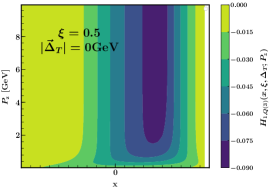
Firstly, we depict the four T-odd GTMD results considering different values of ξ\xi and ΔT\vec{\Delta}_{T} in Figs.1-4. The T-odd GTMD F1o(x,ξ,kT2,ΔT2)F_{1}^{o}(x,\xi,\vec{k}_{T}^{2},\vec{\Delta}_{T}^{2}) as functions of xx and kT\vec{k}_{T} are shown in Fig.1. According to Eq.(26), only in x>ξx>\xi region, the T-odd GTMD has nonvanishing value. In the upper, left panel of Fig.1, we plot the T-odd GTMD F1o(x,ξ,kT2,ΔT2)F_{1}^{o}(x,\xi,\vec{k}_{T}^{2},\vec{\Delta}_{T}^{2}) at ξ=0.1\xi=0.1 and |ΔT|=0|\vec{\Delta}_{T}|=0. Note that in this case the result of F1o(x,ξ,kT2,ΔT2)F_{1}^{o}(x,\xi,\vec{k}_{T}^{2},\vec{\Delta}_{T}^{2}) is negative. One can also find that as the xx value becomes larger, the maximum value of kTk_{T} resulting in nonvanishing F1o(x,ξ,kT2,ΔT2)F_{1}^{o}(x,\xi,\vec{k}_{T}^{2},\vec{\Delta}_{T}^{2}) becomes smaller and at x=0.1x=0.1, the maximum value of kTk_{T} is about 0.8GeV. For a fixed xx value, as the value of kTk_{T} increases, the F1o(x,ξ,kT2,ΔT2)F_{1}^{o}(x,\xi,\vec{k}_{T}^{2},\vec{\Delta}_{T}^{2}) result becomes smaller first and then larger. At a fixed value x=0.1x=0.1, the F1o(x,ξ,kT2,ΔT2)F_{1}^{o}(x,\xi,\vec{k}_{T}^{2},\vec{\Delta}_{T}^{2}) reachs the minimum when kTk_{T} is about 0.3. We depict the F1o(x,ξ,kT2,ΔT2)F_{1}^{o}(x,\xi,\vec{k}_{T}^{2},\vec{\Delta}_{T}^{2}) at ξ=0.1\xi=0.1 and |ΔT|=0.5|\vec{\Delta}_{T}|=0.5 in the upper, right panel of Fig.1. Roughly speaking, it can be seen that the xx-kTk_{T} regions below straight line y=0.25x+0.2y=-0.25x+0.2 are related to positive F1o(x,ξ,kT2,ΔT2)F_{1}^{o}(x,\xi,\vec{k}_{T}^{2},\vec{\Delta}_{T}^{2}). Then we compare the two upper panels in Fig.1 and find that the F1o(x,ξ,kT2,ΔT2)F_{1}^{o}(x,\xi,\vec{k}_{T}^{2},\vec{\Delta}_{T}^{2}) result in the right panel is larger than that in the left panel at the same xx-kTk_{T} point. Comparing the upper panels with the lower panels, we emphasize that the two corresponding contours at x>0.5x>0.5 have nearly the same shape.

Refer to caption
Refer to caption
Figure 4: The T-odd GTMD H1Δ,o(x,ξ,kT2,ΔT2)H_{1}^{\Delta,o}(x,\xi,\vec{k}_{T}^{2},\vec{\Delta}_{T}^{2}) as functions of xx and |kT||\vec{k}_{T}| for different ξ\xi values. The left and right panels H1Δ,o(x,ξ,kT2,ΔT2)H_{1}^{\Delta,o}(x,\xi,\vec{k}_{T}^{2},\vec{\Delta}_{T}^{2}) at |ΔT|=0.1|\vec{\Delta}_{T}|=0.1 with ξ=0.1\xi=0.1 and 0.50.5, respectively.

Fig.2 depicts the T-odd GTMD G~1o(x,ξ,kT2,ΔT2)\tilde{G}_{1}^{o}(x,\xi,\vec{k}_{T}^{2},\vec{\Delta}_{T}^{2}) as functions of xx and kT\vec{k}_{T}, where the paremeter values of contours are the same as Fig.1. In two left panels, the G~1o(x,ξ,kT2,ΔT2)\tilde{G}_{1}^{o}(x,\xi,\vec{k}_{T}^{2},\vec{\Delta}_{T}^{2}) result increases as xx or kTk_{T} increases. Comparing two left panels, we find that the G~1o(x,ξ,kT2,ΔT2)\tilde{G}_{1}^{o}(x,\xi,\vec{k}_{T}^{2},\vec{\Delta}_{T}^{2}) result in the lower panel is slightly smaller than that in the upper panel at the same xx-kTk_{T} point; While the G~1o(x,ξ,kT2,ΔT2)\tilde{G}_{1}^{o}(x,\xi,\vec{k}_{T}^{2},\vec{\Delta}_{T}^{2}) results in two right panels are usually positive. Unlike two right panels in Fig.1 where we plot contours at |ΔT|=0.5|\vec{\Delta}_{T}|=0.5, we show the result at |ΔT|=0.1|\vec{\Delta}_{T}|=0.1. Such difference indicates that the allowable maximum of |ΔT||\vec{\Delta}_{T}| for reaching nonvanishing T-odd GTMD G~1o(x,ξ,kT2,ΔT2)\tilde{G}_{1}^{o}(x,\xi,\vec{k}_{T}^{2},\vec{\Delta}_{T}^{2}) becomes smaller in terms of that for F1o(x,ξ,kT2,ΔT2)F_{1}^{o}(x,\xi,\vec{k}_{T}^{2},\vec{\Delta}_{T}^{2}). We plot the T-odd GTMD H1k,o(x,ξ,kT2,ΔT2)H_{1}^{k,o}(x,\xi,\vec{k}_{T}^{2},\vec{\Delta}_{T}^{2}) as functions of xx and kT\vec{k}_{T} in Fig.3, where the paremeter values of contours are the same as Fig.1. All four panels basically show the same shape of contours. Moreover, the maximum absolute value of the T-odd GTMD H1k,o(x,ξ,kT2,ΔT2)H_{1}^{k,o}(x,\xi,\vec{k}_{T}^{2},\vec{\Delta}_{T}^{2}) can achieve 0.56 which is a larger value than those in Figs.1-2. In Fig.4, the T-odd GTMD H1Δ,o(x,ξ,kT2,ΔT2)H_{1}^{\Delta,o}(x,\xi,\vec{k}_{T}^{2},\vec{\Delta}_{T}^{2}) as a function of xx and kT\vec{k}_{T} at |ΔT|=0.1|\vec{\Delta}_{T}|=0.1 has been shown. Note that this GTMD becomes zero when |ΔT|=0|\vec{\Delta}_{T}|=0.

Refer to caption
Refer to caption
Refer to caption
Refer to caption
Figure 5: Quasi-TMD h1π,Q(3)(x,kT2;Pz)h_{1\pi,Q(3)}^{\perp}(x,\vec{k}_{T}^{2};P_{z}) as functions of x and |kT||\vec{k}_{T}| at different values of PzP_{z} and TMD h1π(x,kT2)h_{1\pi}^{\perp}(x,\vec{k}_{T}^{2}) as functions of x and |kT||\vec{k}_{T}|. Upper left panel: h1π,Q(3)(x,kT2;Pz)h_{1\pi,Q(3)}^{\perp}(x,\vec{k}_{T}^{2};P_{z}) at Pz=1P_{z}=1GeV. Upper right panel: h1π,Q(3)(x,kT2;Pz)h_{1\pi,Q(3)}^{\perp}(x,\vec{k}_{T}^{2};P_{z}) at Pz=3P_{z}=3GeV. Lower left panel: h1π,Q(3)(x,kT2;Pz)h_{1\pi,Q(3)}^{\perp}(x,\vec{k}_{T}^{2};P_{z}) at Pz=5P_{z}=5GeV. Lower right panel: TMD h1π(x,kT2)h_{1\pi}^{\perp}(x,\vec{k}_{T}^{2}) as functions of x and |kT||\vec{k}_{T}|.

In the following we turn to the results of quasi-TMD h1π,Q(3)h_{1\pi,Q(3)}^{\perp} and quasi-GPD H1,Q(3)H_{1,Q(3)}. In Fig.5, we plot the quasi-TMD h1π,Q(3)(x,kT2;Pz)h_{1\pi,Q(3)}^{\perp}(x,\vec{k}_{T}^{2};P_{z}) as functions of xx and kTk_{T} at different values of PzP_{z} and TMD h1π(x,kT2)h_{1\pi}^{\perp}(x,\vec{k}_{T}^{2}) as functions of xx and kTk_{T}. We can see from the upper left panel that the absolute value of quasi-TMD h1π,Q(3)(x,kT2;Pz)h_{1\pi,Q(3)}^{\perp}(x,\vec{k}_{T}^{2};P_{z}) becomes larger as kTk_{T} close to zero. In some region with negative xx, the corresponding h1π(x,kT2)h_{1\pi}^{\perp}(x,\vec{k}_{T}^{2}) has nonvanishing values. As xx increases from 0.3-0.3 to 11, the resulting h1π(x,kT2)h_{1\pi}^{\perp}(x,\vec{k}_{T}^{2}) absolute value gets larger first and then becomes smaller. For a nonvanishing h1π(x,kT2)h_{1\pi}^{\perp}(x,\vec{k}_{T}^{2}) result, the allowable maximum value of kTk_{T} is around 0.380.38. Comparing the three panels in Fig.5 depicting the quasi-TMD h1π,Q(3)(x,kT2;Pz)h_{1\pi,Q(3)}^{\perp}(x,\vec{k}_{T}^{2};P_{z}) with Pz=1,3,5P_{z}=1,3,5 GeV, we can find that as the PzP_{z} value increases, the minimum of xx inside the contours becomes larger. In the lower left panel with Pz=5P_{z}=5 GeV, the quasi-TMD h1π,Q(3)(x,kT2;Pz)h_{1\pi,Q(3)}^{\perp}(x,\vec{k}_{T}^{2};P_{z}) result stay the same at a fixed kTk_{T} value except the case xx close to 0 or 1. The TMD h1π(x,kT2)h_{1\pi}^{\perp}(x,\vec{k}_{T}^{2}) as a negative function of xx and kTk_{T} is shown in the lower right panel of Fig.5. The absolute value of h1π(x,kT2)h_{1\pi}^{\perp}(x,\vec{k}_{T}^{2}) can reach 0.28 in almost all the xx range at a very small value of kTk_{T}.

Refer to caption
Refer to caption
Refer to caption
Refer to caption
Figure 6: Quasi-GPD H1,Q(3)(x,ξ,ΔT2;Pz)H_{1,Q(3)}(x,\xi,\vec{\Delta}_{T}^{2};P_{z}) as functions of xx and PzP_{z} for different ξ\xi and |ΔT||\vec{\Delta}_{T}| values. The upper and lower panels display H1,Q(3)(x,ξ,ΔT2;Pz)H_{1,Q(3)}(x,\xi,\vec{\Delta}_{T}^{2};P_{z}) at ξ=0.1\xi=0.1 and 0.50.5, respectively. The left and right panels show H1,Q(3)(x,ξ,ΔT2;Pz)H_{1,Q(3)}(x,\xi,\vec{\Delta}_{T}^{2};P_{z}) at |ΔT|=0|\vec{\Delta}_{T}|=0 and 0.50.5, respectively.

Finally, we display the quasi-GPD H1,Q(3)(x,ξ,ΔT2;Pz)H_{1,Q(3)}(x,\xi,\vec{\Delta}_{T}^{2};P_{z}) as functions of xx and PzP_{z} for different ξ\xi and |ΔT||\vec{\Delta}_{T}| values in Fig.6. This quasi-GPD is negative. In the upper left panel, it is desired to mention that when Pz>3P_{z}>3 GeV, the quasi-GPD H1,Q(3)(x,ξ,ΔT2;Pz)H_{1,Q(3)}(x,\xi,\vec{\Delta}_{T}^{2};P_{z}) result hardly depends on the value of PzP_{z}. After comparing the two upper panels, we can acquire that the allowable range of xx for the nonvanishing quasi-GPD H1,Q(3)(x,ξ,ΔT2;Pz)H_{1,Q(3)}(x,\xi,\vec{\Delta}_{T}^{2};P_{z}) becomes larger when |ΔT||\vec{\Delta}_{T}| slightly increases from zero. Two panels have the very similar contour shape. When ξ=0.5\xi=0.5, the quasi-GPD H1,Q(3)(x,ξ,ΔT2;Pz)H_{1,Q(3)}(x,\xi,\vec{\Delta}_{T}^{2};P_{z}) result is shown in two lower panels of Fig.6. The absolute values of H1,Q(3)(x,ξ,ΔT2;Pz)H_{1,Q(3)}(x,\xi,\vec{\Delta}_{T}^{2};P_{z}) in two lower panels are smaller than those in two upper panels. We also find that when Pz>3P_{z}>3 GeV, the quasi-GPD H1,Q(3)(x,ξ,ΔT2;Pz)H_{1,Q(3)}(x,\xi,\vec{\Delta}_{T}^{2};P_{z}) result hardly depends on the value of PzP_{z}.

V Conclusion

In this paper we have computed four T-odd GTMDs, quasi-TMD and quasi-GPD in a scalar spectator model. We have present the results for four T-odd GTMDs. To get nonzero results for these functions requires considering at least one-loop corrections that include effects from the Wilson line. We have studied the relation of GTMDs for different values of skewness ξ\xi defined as the longitudinal momentum transferred to the proton and the total momentum transferred to the proton |ΔT||\vec{\Delta}_{T}|. We found only in x>ξx>\xi region, the T-odd GTMDs has nonvanishing value. Generally, the four T-odd GTMDs are negative in xx-kTk_{T} space. However, the G~1o(x,ξ,kT2,ΔT2)\tilde{G}_{1}^{o}(x,\xi,\vec{k}_{T}^{2},\vec{\Delta}_{T}^{2}) results in certain parameter space are positive. Note that the T-odd GTMD H1Δ,o(x,ξ,kT2,ΔT2)H_{1}^{\Delta,o}(x,\xi,\vec{k}_{T}^{2},\vec{\Delta}_{T}^{2}) becomes zero when |ΔT|=0|\vec{\Delta}_{T}|=0. We have also considered the distributions of quasi-TMD and quasi-GPD. For the contours of quasi-TMD, we can find that as the PzP_{z} value increases, the minimum of xx inside the contours becomes larger. We also find that when Pz>3P_{z}>3 GeV, the quasi-GPD H1,Q(3)(x,ξ,ΔT2;Pz)H_{1,Q(3)}(x,\xi,\vec{\Delta}_{T}^{2};P_{z}) result hardly depends on the value of PzP_{z}.

Acknowledgements.
Hao Sun is supported by the National Natural Science Foundation of China (Grant No.11675033) and by the Fundamental Research Funds for the Central Universities (Grant No. DUT18LK27).

References

  • Diehl (2003) M. Diehl, Phys. Rept. 388, 41 (2003), eprint hep-ph/0307382.
  • Belitsky and Radyushkin (2005) A. V. Belitsky and A. V. Radyushkin, Phys. Rept. 418, 1 (2005), eprint hep-ph/0504030.
  • Garcon (2002) M. Garcon (2002), [Eur. Phys. J.A18,389(2003)], eprint hep-ph/0210068.
  • Goeke et al. (2001) K. Goeke, M. V. Polyakov, and M. Vanderhaeghen, Prog. Part. Nucl. Phys. 47, 401 (2001), eprint hep-ph/0106012.
  • Collins and Soper (1982) J. C. Collins and D. E. Soper, Nucl. Phys. B194, 445 (1982).
  • Bacchetta et al. (2007) A. Bacchetta, M. Diehl, K. Goeke, A. Metz, P. J. Mulders, and M. Schlegel, JHEP 02, 093 (2007), eprint hep-ph/0611265.
  • Meissner et al. (2007) S. Meissner, A. Metz, and K. Goeke, Phys. Rev. D76, 034002 (2007), eprint hep-ph/0703176.
  • Meissner et al. (2008) S. Meissner, A. Metz, M. Schlegel, and K. Goeke, JHEP 08, 038 (2008), eprint 0805.3165.
  • Meissner et al. (2009) S. Meissner, A. Metz, and M. Schlegel, JHEP 08, 056 (2009), eprint 0906.5323.
  • Lorcé and Pasquini (2013) C. Lorcé and B. Pasquini, JHEP 09, 138 (2013), eprint 1307.4497.
  • Brodsky et al. (2002) S. J. Brodsky, D. S. Hwang, and I. Schmidt, Phys. Lett. B530, 99 (2002), eprint hep-ph/0201296.
  • Dolgov et al. (2002) D. Dolgov et al. (LHPC, TXL), Phys. Rev. D 66, 034506 (2002), eprint hep-lat/0201021.
  • Gockeler et al. (2005) M. Gockeler, R. Horsley, D. Pleiter, P. E. Rakow, and G. Schierholz (QCDSF), Phys. Rev. D 71, 114511 (2005), eprint hep-ph/0410187.
  • Ji (2013) X. Ji, Phys. Rev. Lett. 110, 262002 (2013), eprint 1305.1539.
  • Ma and Qiu (2018) Y.-Q. Ma and J.-W. Qiu, Phys. Rev. D 98, 074021 (2018), eprint 1404.6860.
  • Ji (2014) X. Ji, Sci. China Phys. Mech. Astron. 57, 1407 (2014), eprint 1404.6680.
  • Lin et al. (2015) H.-W. Lin, J.-W. Chen, S. D. Cohen, and X. Ji, Phys. Rev. D 91, 054510 (2015), eprint 1402.1462.
  • Ji et al. (2020) X. Ji, Y.-S. Liu, Y. Liu, J.-H. Zhang, and Y. Zhao (2020), eprint 2004.03543.
  • Orginos et al. (2017) K. Orginos, A. Radyushkin, J. Karpie, and S. Zafeiropoulos, Phys. Rev. D 96, 094503 (2017), eprint 1706.05373.
  • Green et al. (2018) J. Green, K. Jansen, and F. Steffens, Phys. Rev. Lett. 121, 022004 (2018), eprint 1707.07152.
  • Alexandrou et al. (2015) C. Alexandrou, K. Cichy, V. Drach, E. Garcia-Ramos, K. Hadjiyiannakou, K. Jansen, F. Steffens, and C. Wiese, Phys. Rev. D 92, 014502 (2015), eprint 1504.07455.
  • Chen et al. (2016) J.-W. Chen, S. D. Cohen, X. Ji, H.-W. Lin, and J.-H. Zhang, Nucl. Phys. B 911, 246 (2016), eprint 1603.06664.
  • Alexandrou et al. (2017a) C. Alexandrou, K. Cichy, M. Constantinou, K. Hadjiyiannakou, K. Jansen, F. Steffens, and C. Wiese, Phys. Rev. D 96, 014513 (2017a), eprint 1610.03689.
  • Zhang et al. (2017) J.-H. Zhang, J.-W. Chen, X. Ji, L. Jin, and H.-W. Lin, Phys. Rev. D 95, 094514 (2017), eprint 1702.00008.
  • Lin et al. (2018a) H.-W. Lin, J.-W. Chen, T. Ishikawa, and J.-H. Zhang (LP3), Phys. Rev. D 98, 054504 (2018a), eprint 1708.05301.
  • Bali et al. (2018) G. S. Bali et al., Eur. Phys. J. C 78, 217 (2018), eprint 1709.04325.
  • Alexandrou et al. (2018a) C. Alexandrou, S. Bacchio, K. Cichy, M. Constantinou, K. Hadjiyiannakou, K. Jansen, G. Koutsou, A. Scapellato, and F. Steffens, EPJ Web Conf. 175, 14008 (2018a), eprint 1710.06408.
  • Zhang et al. (2019a) J.-H. Zhang, L. Jin, H.-W. Lin, A. Schäfer, P. Sun, Y.-B. Yang, R. Zhang, Y. Zhao, and J.-W. Chen (LP3), Nucl. Phys. B 939, 429 (2019a), eprint 1712.10025.
  • Alexandrou et al. (2018b) C. Alexandrou, K. Cichy, M. Constantinou, K. Jansen, A. Scapellato, and F. Steffens, Phys. Rev. Lett. 121, 112001 (2018b), eprint 1803.02685.
  • Chen et al. (2018a) J.-W. Chen, L. Jin, H.-W. Lin, Y.-S. Liu, Y.-B. Yang, J.-H. Zhang, and Y. Zhao (2018a), eprint 1803.04393.
  • Zhang et al. (2019b) J.-H. Zhang, J.-W. Chen, L. Jin, H.-W. Lin, A. Schäfer, and Y. Zhao, Phys. Rev. D 100, 034505 (2019b), eprint 1804.01483.
  • Alexandrou et al. (2018c) C. Alexandrou, K. Cichy, M. Constantinou, K. Jansen, A. Scapellato, and F. Steffens, Phys. Rev. D 98, 091503 (2018c), eprint 1807.00232.
  • Liu et al. (2020) Y.-S. Liu et al. (Lattice Parton), Phys. Rev. D 101, 034020 (2020), eprint 1807.06566.
  • Lin et al. (2018b) H.-W. Lin, J.-W. Chen, X. Ji, L. Jin, R. Li, Y.-S. Liu, Y.-B. Yang, J.-H. Zhang, and Y. Zhao, Phys. Rev. Lett. 121, 242003 (2018b), eprint 1807.07431.
  • Gamberg et al. (2015) L. Gamberg, Z.-B. Kang, I. Vitev, and H. Xing, Phys. Lett. B 743, 112 (2015), eprint 1412.3401.
  • Bacchetta et al. (2017) A. Bacchetta, M. Radici, B. Pasquini, and X. Xiong, Phys. Rev. D 95, 014036 (2017), eprint 1608.07638.
  • Nam (2017) S.-i. Nam, Mod. Phys. Lett. A 32, 1750218 (2017), eprint 1704.03824.
  • Broniowski and Ruiz Arriola (2017) W. Broniowski and E. Ruiz Arriola, Phys. Lett. B 773, 385 (2017), eprint 1707.09588.
  • Hobbs (2018) T. Hobbs, Phys. Rev. D 97, 054028 (2018), eprint 1708.05463.
  • Broniowski and Ruiz Arriola (2018) W. Broniowski and E. Ruiz Arriola, Phys. Rev. D 97, 034031 (2018), eprint 1711.03377.
  • Xu et al. (2018) S.-S. Xu, L. Chang, C. D. Roberts, and H.-S. Zong, Phys. Rev. D 97, 094014 (2018), eprint 1802.09552.
  • Chen et al. (2018b) J.-W. Chen, T. Ishikawa, L. Jin, H.-W. Lin, Y.-B. Yang, J.-H. Zhang, and Y. Zhao, Phys. Rev. D 97, 014505 (2018b), eprint 1706.01295.
  • Ji et al. (2018) X. Ji, J.-H. Zhang, and Y. Zhao, Phys. Rev. Lett. 120, 112001 (2018), eprint 1706.08962.
  • Ishikawa et al. (2017) T. Ishikawa, Y.-Q. Ma, J.-W. Qiu, and S. Yoshida, Phys. Rev. D 96, 094019 (2017), eprint 1707.03107.
  • Alexandrou et al. (2017b) C. Alexandrou, K. Cichy, M. Constantinou, K. Hadjiyiannakou, K. Jansen, H. Panagopoulos, and F. Steffens, Nucl. Phys. B 923, 394 (2017b), eprint 1706.00265.
  • Constantinou and Panagopoulos (2017) M. Constantinou and H. Panagopoulos, Phys. Rev. D 96, 054506 (2017), eprint 1705.11193.
  • Xiong et al. (2017) X. Xiong, T. Luu, and U.-G. Meißner (2017), eprint 1705.00246.
  • Chen et al. (2017) J.-W. Chen, X. Ji, and J.-H. Zhang, Nucl. Phys. B 915, 1 (2017), eprint 1609.08102.
  • Ishikawa et al. (2016) T. Ishikawa, Y.-Q. Ma, J.-W. Qiu, and S. Yoshida (2016), eprint 1609.02018.
  • Ji et al. (2015) X. Ji, P. Sun, X. Xiong, and F. Yuan, Phys. Rev. D91, 074009 (2015), eprint 1405.7640.
  • Ji et al. (2019a) X. Ji, L.-C. Jin, F. Yuan, J.-H. Zhang, and Y. Zhao, Phys. Rev. D 99, 114006 (2019a), eprint 1801.05930.
  • Ebert et al. (2019a) M. A. Ebert, I. W. Stewart, and Y. Zhao, Phys. Rev. D99, 034505 (2019a), eprint 1811.00026.
  • Ebert et al. (2019b) M. A. Ebert, I. W. Stewart, and Y. Zhao, JHEP 09, 037 (2019b), eprint 1901.03685.
  • Ebert et al. (2020a) M. A. Ebert, I. W. Stewart, and Y. Zhao, JHEP 03, 099 (2020a), eprint 1910.08569.
  • Ji et al. (2019b) X. Ji, Y. Liu, and Y.-S. Liu (2019b), eprint 1910.11415.
  • Ji et al. (2019c) X. Ji, Y. Liu, and Y.-S. Liu (2019c), eprint 1911.03840.
  • Vladimirov and Schäfer (2020) A. A. Vladimirov and A. Schäfer, Phys. Rev. D101, 074517 (2020), eprint 2002.07527.
  • Ebert et al. (2020b) M. A. Ebert, S. T. Schindler, I. W. Stewart, and Y. Zhao (2020b), eprint 2004.14831.
  • Shanahan et al. (2020a) P. Shanahan, M. L. Wagman, and Y. Zhao, Phys. Rev. D101, 074505 (2020a), eprint 1911.00800.
  • Shanahan et al. (2020b) P. Shanahan, M. Wagman, and Y. Zhao (2020b), eprint 2003.06063.
  • Bhattacharya et al. (2019a) S. Bhattacharya, C. Cocuzza, and A. Metz, Phys. Lett. B 788, 453 (2019a), eprint 1808.01437.
  • Bhattacharya et al. (2019b) S. Bhattacharya, C. Cocuzza, and A. Metz (2019b), eprint 1903.05721.
  • Ma et al. (2019) Z.-L. Ma, J.-Q. Zhu, and Z. Lu (2019), eprint 1912.12816.
  • Broniowski and Ruiz Arriola (2003) W. Broniowski and E. Ruiz Arriola, Phys. Lett. B574, 57 (2003), eprint hep-ph/0307198.
  • Dorokhov et al. (2011) A. E. Dorokhov, W. Broniowski, and E. Ruiz Arriola, Phys. Rev. D84, 074015 (2011), eprint 1107.5631.
  • Davidson and Ruiz Arriola (2002) R. M. Davidson and E. Ruiz Arriola, Acta Phys. Polon. B33, 1791 (2002), eprint hep-ph/0110291.
  • Theussl et al. (2004) L. Theussl, S. Noguera, and V. Vento, Eur. Phys. J. A20, 483 (2004), eprint nucl-th/0211036.
  • Frederico et al. (2009) T. Frederico, E. Pace, B. Pasquini, and G. Salme, Phys. Rev. D80, 054021 (2009), eprint 0907.5566.
  • Brömmel et al. (2008) D. Brömmel et al. (QCDSF, UKQCD), Phys. Rev. Lett. 101, 122001 (2008), eprint 0708.2249.
  • Sufian et al. (2020) R. S. Sufian, C. Egerer, J. Karpie, R. G. Edwards, B. Joó, Y.-Q. Ma, K. Orginos, J.-W. Qiu, and D. G. Richards (2020), eprint 2001.04960.
  • Izubuchi et al. (2019) T. Izubuchi, L. Jin, C. Kallidonis, N. Karthik, S. Mukherjee, P. Petreczky, C. Shugert, and S. Syritsyn, Phys. Rev. D100, 034516 (2019), eprint 1905.06349.
  • Chen et al. (2019) J.-W. Chen, H.-W. Lin, and J.-H. Zhang (2019), eprint 1904.12376.
  • Barone et al. (2010) V. Barone, F. Bradamante, and A. Martin, Prog. Part. Nucl. Phys. 65, 267 (2010), eprint 1011.0909.
  • Boer and Mulders (1998) D. Boer and P. Mulders, Phys. Rev. D 57, 5780 (1998), eprint hep-ph/9711485.
  • Radyushkin (2017) A. Radyushkin, Phys. Lett. B 767, 314 (2017), eprint 1612.05170.
  • Gluck et al. (1992) M. Gluck, E. Reya, and A. Vogt, Z. Phys. C53, 651 (1992).
  • Lu and Ma (2004) Z. Lu and B.-Q. Ma, Phys. Rev. D70, 094044 (2004), eprint hep-ph/0411043.
  • Burkardt and Hannafious (2008) M. Burkardt and B. Hannafious, Phys. Lett. B 658, 130 (2008), eprint 0705.1573.