System III: Learning with Domain Knowledge for Safety Constraints

While existing Reinforcement Learning (RL) methods provide promising guarantees given sufficient exploration guarantees, in safety-critical applications most of the exploration methods are impractical due to the system vulnerability. Consider the example of a self-driving car where the controller agent should respect the speed limit, should not cross the stop sign, and should not crash into objects and other agents in the environment [2]. Safety in RL is not limited to self-driving cars, it can be used to make algorithms systematically safe and aligned with human intent [17]. In safety-critical domains such as autonomous driving, warehouse logistics or assistance in health care, experts require deep RL controllers to operate within known bounds and limits. Let us refer to these safety bounds and limits as constraints. Recent advances in the development of deep RL provide means to allow prior domain knowledge to be encoded in the training processes of neural networks. However, previous efforts on encoding the constraints requires direct modification of the optimization problem. Specifically, the constraints are encoded in the loss function, which may require heavy domain-specific engineering [8]. Consequently, these approaches are not suitable in safety-critical domains where the constraints must be satisfied during learning and thus sample efficiency is an important factor. Although combining expert constraints with neural networks tends to help learning, generating expert constraints remains challenging, understudied and domain-dependent. Further related work is discussed in Appendix 2.

In this work we take inspiration from [7, 20, 27] and express our constrains in first-order logic, which allows for efficient encoding of expert domain knowledge. Deep reinforcement learning relies on extensive exploration to generate data, which is highly undesirable when dealing with safety-critical domains. On the other hand, exploration is needed in order to learn and generalize better.

In this paper, we address both issues. Firstly, we provide a novel way of incorporating constraints in the training processes of deep reinforcement learning. We do not manipulate the current deep learning formulations, i.e. we do not add any extra regularization parameter in the loss function, nor do we rely on any domain-specific engineering. Our approach evaluates the likelihood of constraints being satisfied at each point in time given a state prediction, and this affects the agent’s reward function. Namely, actions that highly satisfy the constraints are encouraged, and actions that do not fully satisfy the constraints are discouraged. Secondly, we use model-based reinforcement learning techniques, which are data-efficient comparing to model-free counterparts. In general, the proposed approach can be seen as analogous to combining system I and system II of the brain, as discussed in Kahneman’s Thinking Fast and Slow [18]. Whilst system I is fast, automatic and intuitive, system II is slower, analytical, and has reasoning capabilities. Hence, we call this approach "System III" as we represent logical constraints and combine them with the high-performing fast deep learning algorithms.

To show the effectiveness of System III, we conduct experiments on classic control tasks such as the Cart-Pole setup from OpenAI’s Gym [3], which is a common task in many reinforcement learning algorithms. We show that even a simple constraint on the Cart-Pole system leads to safer exploration and faster convergence. We further conduct experiments on the OpenAI Safety-Gym environments [1]. We show the approach’s superiority in safe exploration for a wide arrangement of constraints, hazards and environment configuration in a dynamic setting where the constraints differ across experiments. Further details are discussed in Section 8. The contribution of this paper is a novel framework for integrating domain knowledge in the training process of deep RL. Our framework is applicable to any off-the-shelf reinforcement learning algorithm and can be used on top of them to encode domain knowledge and boost sample efficiency significantly while satisfying the constraints.

In this section, we compare supervised, unsupervised and RL related works that use human knowledge in the form of constraints. The integration of constraints as an additional regularizer in the training process of neural networks has achieved considerable attention in recent years, with most work still imposing constraints on the network’s output [27, 7]. The main contribution of "Semantics loss" [27] is the addition of a semantic loss function to the standard neural network loss (e.g. another regularizer), and the design is such that it is equivalent to evaluating some Boolean constraint formula using Weighted Model Counting (WMC) which counts the weights of the solutions to a propositional logic formula [6]. Similar to [27], [7] defines a non-negative loss function using fuzzy logic to incorporate logical constraints. This loss measures how far the output of the network is from the nearest satisfying solution. Our approach differs from both of these. We compile constraints and add them to the training process of an RL agent; our constraints are motivated by real-world physics, which are crucial for safety-critical domains. Unlike [27] we do not rely on WMC to evaluate the constraints as they rely on SAT solvers, instead we designed a more suitable metric for constraint evaluation in sequential decision-making tasks.

One of the closest works to ours is [28] comprised of a two-system, a fuzzy rule controller that takes the represented human knowledge constraints and returns a preferred action and a refined module that tunes the suboptimal knowledge. The constraints are represented in fuzzy logic and allow for imprecise policy selection. During the constraint generation, they assume to have perfect knowledge of the state-space, and the constraints fully capture all aspects of the state-space, which is a strong assumption to hold. Our work differs from this: we do not assume to know the full-state space dynamics and do not use constraints to warm-start the policy; further, our constraints are much more general and expressive. To illustrate this generality, consider the rule from [28] Rule: IF $S_{1}$ is $Ml_{1}$ and $S_{2}$ is $Ml_{2}$ and… and $S_{k}$ is $Ml_{k}$ THEN Action is $a_{j}$: where $S_{i}$ are variables that describe different parts of the state, $Ml_{i}$ is the fuzzy rules corresponding to each $S_{i}$ and $a_{j}$ is the action taken. This rule would only be applicable with in fully observable scenarios: an assumption which is unrealistic in many real-world applications. Their approach is no different to hard encoding actions. In our framework, constraints are high level, general, and provide expressiveness. For example, consider when we want to specify that the agent’s distance to an undesired object (e.g. traffic light) should be greater than the lower bound or if the distance is less than, the lower bound, the agent should decrease its speed $\varphi(s)=(lb\leq||s-obj||)\lor(velocity\leq v_{limit}\land||s-obj||\leq ub)$. Similarly, there exist other approaches [9, 11, 13, 10, 16, 12, 14, 5, 15] that define safety by the satisfaction of temporal logical formulae of the learnt policy.

Other works in this space [19] propose constrained Q-learning to restrict the action space directly in the Q-update to learn the optimal Q-function; they claim this approach can lead to optimal safe policy in the induced MDP. Our method also differs from this approach, and we do not change anything in the existing deep RL toolbox. However, we believe that some actions become prohibited in our constraint evaluation phase due to low log probability.

In this section, we introduce RL formalism and model-based RL methods that we will build upon in the development of System III. We model our problem as Markov Decision Process (MDP), which is defined as a tuple $\langle S,A,P,R,\gamma\rangle$. In the MDP model $S\subseteq\mathbb{R}^{n}$ is a continuous state space, $A\subseteq\mathbb{R}^{m}$ is a continuous action space, and $P:\mathfrak{B}(\mathbb{R}^{n})\times A\times S\rightarrow[0,1]$ is a Borel-measurable conditional transition kernel such that $P(\cdot|s,a)$ is a probability measure of $s\in S$ and $a\in A$ over the Borel space $(\mathbb{R}^{n},\mathfrak{B}(\mathbb{R}^{n}))$, where $\mathfrak{B}(\mathbb{R}^{n})$ is the set of all Borel sets on $\mathbb{R}^{n}$. The transition probability $P$ captures the motion uncertainties of the agent, and it is assumed that $P$ is not known a priori. A reward function $R:S\times A\times S\rightarrow\mathbb{R}$ defines a scalar feedback that the agent receives. At each time step $t$ in the environment, the agent observes a state $s_{t}\in S$, executes an action $a_{t}\in A$ and transitions to the next state $s_{t+1}\sim P(\cdot|s_{t},a_{t})$ and receives the reward associated with that action $r_{t}=R(s_{t},a_{t},s_{t+1})$. The discount factor $\gamma\in[0,1]$ is used to weigh the current value of future returns. A policy $\pi$ is a mapping from the state space to a distribution in $\mathcal{P}(\mathcal{A})$, where $\mathcal{P}(\mathcal{A})$ is the set of probability distributions on subsets of $\mathcal{A}$. A policy is stationary if $\pi(\cdot|s)\in\mathcal{P}(\mathcal{A})$ does not change over time and it is called a deterministic policy if $\pi(\cdot|s)$ is a degenerate distribution. The objective in RL is to find a policy $\pi^{*}$ that maximises the expected discounted sum of rewards,

where $a_{t}\sim\pi(\cdot|s_{t})$, and $s_{t+1}\sim P(\cdot|s,a)$ [25, 22]. The value of state $s$ under any policy $\pi$, denoted as $V^{\pi}(s)$, is similarly defined as the expected return starting at state $s$ and following $\pi$ afterwards: $V^{\pi}(s)=\mathbb{E}_{\pi}\Big{[}\sum_{t=0}^{\infty}\gamma^{t}r_{t}\mid s_{0}=s\Big{]}.$ We might drop $\pi$ to simplify notation. We focus on policy gradient methods, which model and optimise the policy directly. Different policy gradient-based algorithms have been proposed in the literature, e.g., TRPO [23] and ACKTR [26], that learn to update the policy subject to a constraint in the policy space which discourages large differences between successive policies.

In policy gradient techniques, the key idea is to increase the probability of actions that are associated with higher returns and reduce the probability of actions that lead to lower return until an optimal policy is found. In this paper, we use Asynchronous Advantage Actor Critic policy gradient (A3C) for policy learning [21] combined with Generalized Advantage Estimation (GAE) [24]. For a policy $\pi_{\theta}$ where $\theta$ is the neural network parameters. $J(\pi_{\theta})$ is the expected discounted return, and $\nabla_{\theta}J(\pi_{\theta})$ is the gradient of the return with respect to the $\theta$: $\nabla_{\theta}J(\pi_{\theta})=\mathbb{E_{\pi_{\theta}}}\Big{[}\sum\nabla_{\theta}\log\pi_{\theta}(s,a)A^{\pi_{\theta}}(s,a)\Big{]},$ where $A^{\pi_{\theta}}(s,a)$ is the advantage function. The policy gradient algorithm updates the policy network parameter by stochastic gradient ascent $\theta\leftarrow\theta+\alpha\nabla_{\theta}J(\pi_{\theta})$, where $\alpha$ is the learning rate.

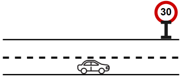
To illustrate how human prior knowledge is mapped to first order logic (FL) sentences, consider the example of driving a car, where a learner, i.e. agent, sits in the driver’s seat and observes the constraints in the environment, e.g. other cars, designated driving lane, speed limit, humans, traffic signs etc. Prior to driving, they have prior knowledge about the constraints in the environment, for example, not to crash into humans, traffic signs, and not to get out of the designated lane. Let us consider the example of not getting out of the designated driving lane and maintaining the speed limit, as shown in Figure 1(a) in Appendix 5. The prior knowledge for keeping the car in its appropriate lane and respecting the speed limit can be expressed in the form of ($lb\leq$ SPEED LIMIT $\leq ub$) $\land$ ($lb^{\prime}\leq$ DESIGNATED LANE $\leq ub^{\prime}$) defined by a desirable range in Conjunctive Normal Form (CNF) or Disjunctive Normal Form (DNF). For instance, if the car speed and the designated lane are in the allowed range, and the distance by which any action moves the car is smaller then the allowed range, any meditate should satisfy the constraint because the agent will still be in the desired range.

Slippery grid world example below:

High-Level FL Constraint: We take motivation from real-world settings, where expressive yet intuitive constraints are required to fully capture the desired behavior while are easily understandable for humans. For example, consider the task of parking between two objects. Formally, given the agent state $s$, the FL constraint is:

where $||s-\mathit{object_{i}}||$ is the agent’s distance to the objects while $lb^{\prime}$ is the lower bound on the distance.

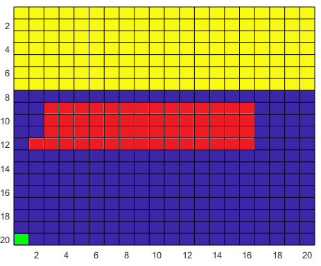
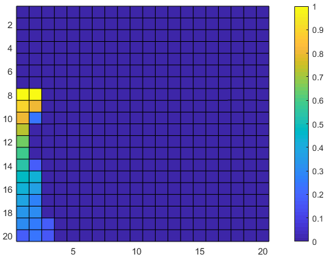
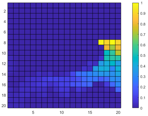
The Running Example is shown in Figure 2 in Appendix 6 and is a moving robot in a grid. Let the grid be a $20\times 20$ square over which the robot moves. In this setup, the robot location is the MDP state $s\in{S}$. At each state $s\in{S}$ the robot has a set of actions ${A}=\{\mathit{left},\mathit{right},\mathit{up},\mathit{down},\mathit{stay}\}$ using which the robot is able to move to other states (e.g. $s^{\prime}$) with the probability of $P(s,a,s^{\prime}),a\in\mathcal{A}$. At each state $s\in{S}$, the actions available to the robot are either to move to a neighbour state $s^{\prime}\in{S}$ or to stay at the state $s$. In this example, we assume for each action the robot chooses, there is a probability of $85\%$ that the action takes the robot to the correct state and $15\%$ that the action takes the robot to a random state in its neighbourhood, including its current state. The property of interest in this example is an FL formula: $\varphi(s)=\forall~{}\mathit{unsafe}_{i}:~{}||s-\mathit{unsafe}_{i}||\leq lb$, where $||s-\mathit{unsafe}_{i}||$ is the agent’s distance to any unsafe (red) state $\mathit{unsafe}_{i}$.

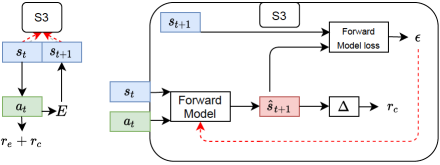
System III architecture: System III comprises two reciprocating subsystems: a system that learns to model the next state $s_{t+1}$ and a system that evaluates the constraints on $s_{t+1}$. The ability of the latter subsystem to evaluate the constraints depends on the former subsystem’s ability to accurately model the next state. We further define the total reward $r_{t}$ to be the sum of reward returned by the environment ($r^{e}_{t}$) and reward returned by the degree of constraints satisfaction ($r^{c}_{t}$) resulting in: $r_{t}={r^{e}_{t}}+{r^{c}_{t}}$.

We use a policy $\pi(\cdot|s_{t};\theta_{p})$ representing an actor neural network, where $s_{t}$ is the current state, and $\theta_{p}$ refers to the weights of the network. An agent at state $s_{t}$ takes the action $a_{t}\sim\pi(\cdot|s_{t};\theta_{p})$ sampled from the policy. The parameters of the policy network $\theta_{p}$ are optimised to maximize the sum of discounted expected return in (1). In order to ensure that the agent explores the state space sufficiently to learn and satisfy the necessary constraints, we construct a model to take as input the state $s_{t}$ and action $a_{t}$ and returns the distribution of next state at $t+1$. This is also known as forward dynamics. Formally: ${\hat{s}_{t+1}}\sim f(\cdot|s_{t},a_{t};\theta_{F})$, where $\hat{s}_{t+1}$ is the estimate of ${s}_{t+1}$ and $\theta_{F}$ is the forward model (e.g. a neural network) parameters. From the forward dynamics we optimize the parameter $\theta_{F}$ by minimizing the mean squared loss function:

With the model $f$ trained via mean squared loss function , we can evaluate the constraints satisfaction at each time step. Consider the running example FL constraint $\varphi(s)=lb\leq||s-\mathit{unsafe}||$. Define $\Delta:S\times A\times S\rightarrow\mathbb{R}$ as the constraint evaluation function. At each time step $t$, the agent observes a state $s_{t}\in S$, chooses an action $a_{t}\in A$ and the forward model $f$ outputs ${\hat{s}_{t+1}}\sim f(\cdot|s_{t},a_{t};\theta_{F})$. The constraint reward is then defined as:

${r^{c}_{t}}=\Delta(s_{t},a_{t},\hat{s}_{t+1})=\begin{cases}1~{}~{}~{}~{}\text{if}~{}~{}\varphi(\hat{s}_{t+1})\\ 0~{}~{}~{}~{}\text{otherwise}\end{cases}$.

We can write the overall optimization problem as a combination of (1) and (2):

where $0\leq\beta\leq 1$ is a scalar that weighs the forward model loss and $\lambda>0$ is a scalar that weighs the importance of the policy gradient loss against the importance of satisfying the constraint.

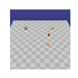
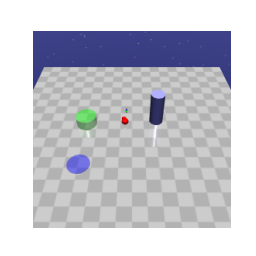
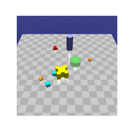
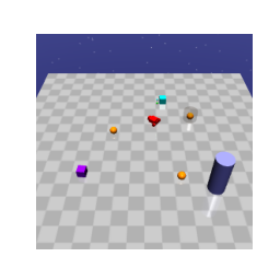
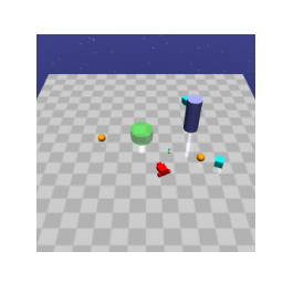
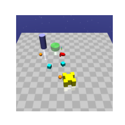
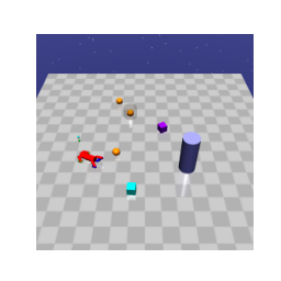
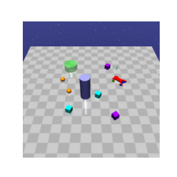
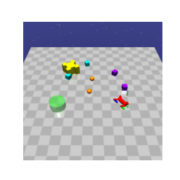
In the running example, in order to get to the target state the agent has to cross a bridge (Fig. 2a) surrounded by unsafe states. The grid is slippery, namely from the agent’s perspective, when it takes an action it usually moves to the intended cell, but there is an unknown probability that the agent is moved to a random neighbour cell. However, the trained model $\hat{P}$ initially advises the agent that it can always move to the correct state and this is the dynamics known to the agent. The initial state of the agent is bottom left. For the simulated physical environments we consider OpenAI Gym [4] and Safety Gym [1]. OpenAI’s Gym environment comprises a set of toolkits for developing and comparing reinforcement learning algorithms. It contains tasks ranging from control to Attari. For this paper, we focus on the continuous control task CartPole [25]. In Safety Gym, we run experiments using the Point, Car and Doggo robot [1] while varying the number of constraints in the environment with constant goal task. In both environments, the agent interacts with the environment and is rewarded based on the degree to which it satisfies the constraints. We leave the case for sparse reward setting for future work. Consider Figure 4(a), where the agent task is to press the highlighted button while avoiding hazards. We represent such scenario via a general FL formula: $\varphi(s)=\{(\forall~{}{\mathit{hazard}_{i}}:lb_{h}\leq||s-\mathit{hazard}_{i}||\leq max\_distance\_pair\_button)\land\\ (\forall~{}{\mathit{goal\_button}_{i}}:||s-\mathit{goal\_button}_{i}||\leq max\_distance\_pair\_button)\}.$

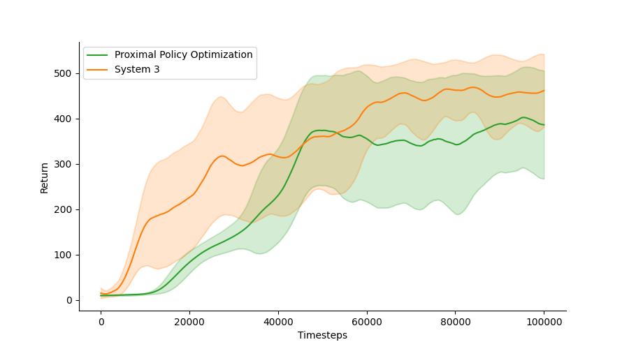
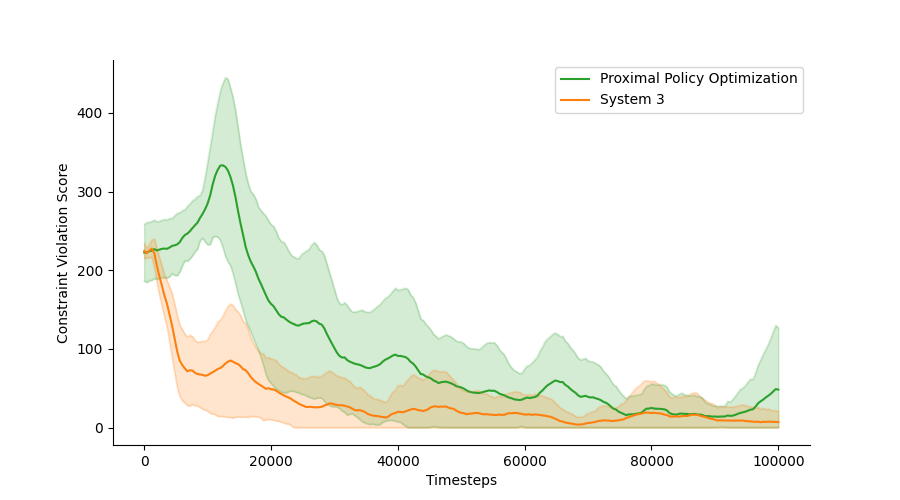
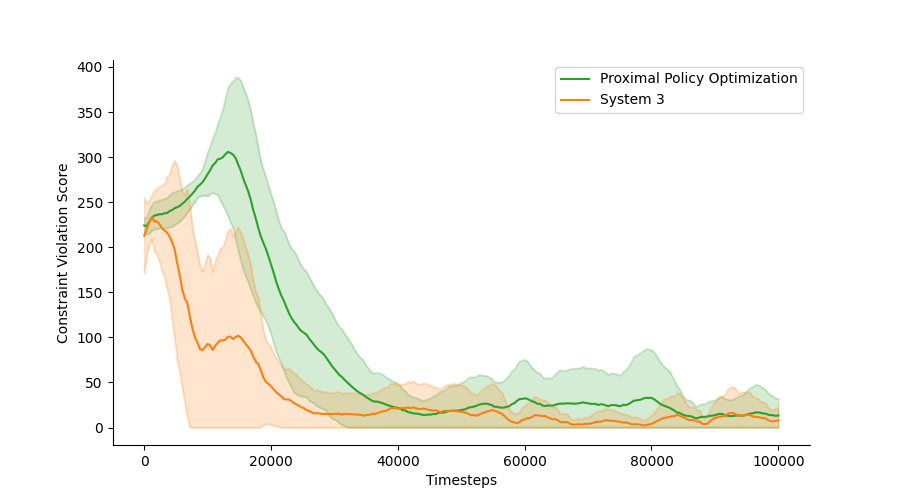
Constraints are defined as an ’allowable’ subspace of the state space. In the CartPole experiment we deliver $d$-step accumulated reward every $d$ time steps. The constraints on the in CartPole is: $\varphi(s)=(lb\leq x\leq ub)\land(lb\leq k\leq ub)$ where $x$ corresponds to the cart position, and $k$ corresponds to the pole angle at tip. We evaluate our algorithm under different delayed steps. Figure 3 plots the results under a sparse reward setting. Similarly, in Safety-Gym, we provide $r^{c}_{t}$ after each immediate action and $r^{e}_{t}$ is fully ignored as $r^{c}_{t}$ captures the degree of satisfaction in each state. Table 1 shows the average episodic mean return along with constraint violation (i.e. 1 - constraint satisfaction), where $0$ corresponds to $0\%$ constraint satisfaction and $1$ corresponds to $100\%$ satisfaction at evaluation. We train our system’s combined objective in 3 with $\lambda$ = 0.15, $\beta$ = 0.3 and learning rate of $1e^{-3}$. We observe there to exist an inverse relationship between the reward and constraint satisfaction. Unconstrained algorithms (e.g. PPO and TRPO) achieves higher return at the cost of high degree of constraint violation. However, PPO and TRPO’s Lagrangian counter part which follows the adaptive penalty to enforce constraints achieves higher degree of constraint satisfaction. We observe a an inverse relationship between achieving higher reward and acting safely. System 3 is able to act safely after a small amount of interaction with the environment at a cost of slightly lower return compared to the other methods which achieves slightly higher return but does significantly worse at satisfying the constraints. We hypothesis this is due to the nature of the the environment reward function not being able to capture the actual desire of the designer and what it intends it to do. We show that our method achieves high constraint satisfaction (95%) as shown in 1 in Appendix 8, compared to popular baselines designed to deal with constrained MDPs.

In this paper we propose a novel framework for incorporating constraints in the training processes of deep reinforcement learning. Our approach evaluates the likelihood of constraints being satisfied at each point in time given a state prediction, and this affects the agent’s reward function. The future work should consider changing the environments and keeping the constraints constant and learn the constraints directly from the environment. From a novel safety and alignment perspective this work provides a solution for outer alignment, however future research would need to address issues that might arise with inner alignment.

References

- [1] Joshua Achiam Alex Ray and Dario Amodei. Benchmarking safe exploration in deep reinforcement learning, 2019.
- [2] Mariusz Bojarski, Davide Del Testa, Daniel Dworakowski, Bernhard Firner, Beat Flepp, Prasoon Goyal, Lawrence D. Jackel, Mathew Monfort, Urs Muller, Jiakai Zhang, Xin Zhang, Jake Zhao, and Karol Zieba. End to end learning for self-driving cars, 2016.
- [3] Greg Brockman, Vicki Cheung, Ludwig Pettersson, Jonas Schneider, John Schulman, Jie Tang, and Wojciech Zaremba. Openai gym. arXiv preprint arXiv:1606.01540, 2016.
- [4] Greg Brockman, Vicki Cheung, Ludwig Pettersson, Jonas Schneider, John Schulman, Jie Tang, and Wojciech Zaremba. Openai gym, 2016.
- [5] Mingyu Cai, Hosein Hasanbeig, Shaoping Xiao, Alessandro Abate, and Zhen Kan. Modular deep reinforcement learning for continuous motion planning with temporal logic. In International Conference on Intelligent Robots and Systems. IEEE/RSJ, 2021.
- [6] Mark Chavira and Adnan Darwiche. On probabilistic inference by weighted model counting. Artif. Intell., 172(6-7):772–799, 2008.
- [7] Marc Fischer, Mislav Balunovic, Dana Drachsler-Cohen, Timon Gehr, Ce Zhang, and Martin Vechev. DL2: Training and querying neural networks with logic. In 36th International Conference on Machine Learning, ICML 2019, volume 2019-June, pages 3411–3427, 2019.
- [8] Javier Garcıa and Fernando Fernández. A comprehensive survey on safe reinforcement learning. Journal of Machine Learning Research, 16(1):1437–1480, 2015.
- [9] Hosein Hasanbeig, Alessandro Abate, and Daniel Kroening. Logically-constrained reinforcement learning. arXiv preprint arXiv:1801.08099, 2018.
- [10] Hosein Hasanbeig, Alessandro Abate, and Daniel Kroening. Certified reinforcement learning with logic guidance. arXiv preprint arXiv:1902.00778, 2019.
- [11] Hosein Hasanbeig, Alessandro Abate, and Daniel Kroening. Logically-constrained neural fitted q-iteration. AAMAS, 2019.
- [12] Hosein Hasanbeig, Alessandro Abate, and Daniel Kroening. Cautious reinforcement learning with logical constraints. AAMAS, 2020.
- [13] Hosein Hasanbeig, Yiannis Kantaros, Alessandro Abate, Daniel Kroening, George J Pappas, and Insup Lee. Reinforcement learning for temporal logic control synthesis with probabilistic satisfaction guarantees. In 2019 IEEE 58th Conference on Decision and Control (CDC), pages 5338–5343. IEEE, 2019.
- [14] Hosein Hasanbeig, Daniel Kroening, and Alessandro Abate. Deep reinforcement learning with temporal logics. In International Conference on Formal Modeling and Analysis of Timed Systems, pages 1–22. Springer, 2020.
- [15] Hosein Hasanbeig, Daniel Kroening, and Alessandro Abate. LCRL: Certified policy synthesis via logically-constrained reinforcement learning. In International Conference on Quantitative Evaluation of Systems, pages 217–231. Springer, 2022.
- [16] Hosein Hasanbeig, Natasha Yogananda Jeppu, Alessandro Abate, Tom Melham, and Daniel Kroening. DeepSynth: Program synthesis for automatic task segmentation in deep reinforcement learning. In AAAI Conference on Artificial Intelligence. Association for the Advancement of Artificial Intelligence, 2021.
- [17] Dan Hendrycks, Nicholas Carlini, John Schulman, and Jacob Steinhardt. Unsolved problems in ML safety. CoRR, abs/2109.13916, 2021.
- [18] Daniel Kahneman. Thinking, fast and slow. Macmillan, 2011.
- [19] Gabriel Kalweit, Maria Huegle, Moritz Werling, and Joschka Boedecker. Deep constrained q-learning, 2020.
- [20] Robin Manhaeve, Angelika Kimmig, Sebastijan Dumančić, Thomas Demeester, and Luc De Raedt. Deepproblog: Neural probabilistic logic programming. In Advances in Neural Information Processing Systems, volume 2018-Decem, pages 3749–3759, 2018.
- [21] Volodymyr Mnih, Adria Puigdomenech Badia, Mehdi Mirza, Alex Graves, Timothy Lillicrap, Tim Harley, David Silver, and Koray Kavukcuoglu. Asynchronous methods for deep reinforcement learning. In Maria Florina Balcan and Kilian Q. Weinberger, editors, Proceedings of The 33rd International Conference on Machine Learning, volume 48 of Proceedings of Machine Learning Research, pages 1928–1937, New York, New York, USA, 20–22 Jun 2016. PMLR.
- [22] Vitchyr Pong, Shixiang Gu, Murtaza Dalal, and Sergey Levine. Temporal difference models: Model-free deep rl for model-based control, 2020.
- [23] John Schulman, Sergey Levine, Philipp Moritz, Michael I. Jordan, and Pieter Abbeel. Trust region policy optimization. CoRR, abs/1502.05477, 2015.
- [24] John Schulman, Philipp Moritz, Sergey Levine, Michael Jordan, and Pieter Abbeel. High-dimensional continuous control using generalized advantage estimation, 2018.
- [25] Richard S. Sutton and Andrew G. Barto. Reinforcement Learning: An Introduction. The MIT Press, second edition, 2018.
- [26] Yuhuai Wu, Elman Mansimov, Shun Liao, Roger B. Grosse, and Jimmy Ba. Scalable trust-region method for deep reinforcement learning using kronecker-factored approximation. CoRR, abs/1708.05144, 2017.
- [27] Jingyi Xu, Zilu Zhang, Tal Friedman, Yitao Liang, and Guy Van den Broeck. A semantic loss function for deep learning with symbolic knowledge. In Jennifer Dy and Andreas Krause, editors, Proceedings of the 35th International Conference on Machine Learning, volume 80 of Proceedings of Machine Learning Research, pages 5502–5511. PMLR, 10–15 Jul 2018.
- [28] Peng Zhang, Jianye Hao, Weixun Wang, Hongyao Tang, Yi Ma, Yihai Duan, and Yan Zheng. Kogun: Accelerating deep reinforcement learning via integrating human suboptimal knowledge. In Christian Bessiere, editor, Proceedings of the Twenty-Ninth International Joint Conference on Artificial Intelligence, IJCAI 2020, pages 2291–2297. ijcai.org, 2020.
Appendix
Appendix A OpenAI SafetyGym