Synthetic Health-related
Longitudinal Data with Mixed-type Variables
Generated using Diffusion Models
Abstract
This paper presents a novel approach to simulating electronic health records (EHRs) using diffusion probabilistic models (DPMs). Specifically, we demonstrate the effectiveness of DPMs in synthesising longitudinal EHRs that capture mixed-type variables, including numeric, binary, and categorical variables. To our knowledge, this represents the first use of DPMs for this purpose. We compared our DPM-simulated datasets to previous state-of-the-art results based on generative adversarial networks (GANs) for two clinical applications: acute hypotension and human immunodeficiency virus (ART for HIV). Given the lack of similar previous studies in DPMs, a core component of our work involves exploring the advantages and caveats of employing DPMs across a wide range of aspects. In addition to assessing the realism of the synthetic datasets, we also trained reinforcement learning (RL) agents on the synthetic data to evaluate their utility for supporting the development of downstream machine learning models. Finally, we estimated that our DPM-simulated datasets are secure and posed a low patient exposure risk for public access.
Keywords: Machine Learning, Synthetic Data,
Generative Adversarial Networks, Diffusion Porbabilistic Models,
Hypotension, ART for HIV
Ethics Statement
This study was approved by the University of New South Wales’ human research ethics committee (application HC210661). We based our synthetic acute hypotension dataset on MIMIC-III (Johnson et al., 2016), and our synthetic HIV dataset on EuResist (Zazzi et al., 2012). For patients in MIMIC-III requirement for individual consent was waived because the project did not impact clinical care and all protected health information was deidentified (Johnson et al., 2016). For people in the EuResist integrated database, all data providers obtained informed consent for the execution of retrospective studies and inclusion in merged cohorts (Prosperi et al., 2010).
1 Introduction
Healthcare data is a crucial resource for the advancement of machine learning (ML) algorithms, including the field of reinforcement learning (RL) (Sutton & Barto, 2018). RL is trained to learn an optimal behaviour policy to match actions (i.e., treatment selections) to the environment (i.e., a patient’s clinical state); and it has the potential to significantly improve healthcare (Komorowski et al., 2018). However, privacy regulations (see Nosowsky & Giordano (2006), O’Keefe & Connolly (2010), and Bentzen et al. (2021)) restrict the use of health-related data, limiting the availability of real-world datasets for research. This scarcity of data negatively impacts the development of ML algorithms, as they require large, diversified datasets to effectively learn and improve. Synthetic data, generated through the use of generative models, offers a solution to this challenge (Kuo et al., 2022b) . By creating highly realistic synthetic datasets, the research community can develop, test, and compare ML algorithms in a controlled environment, without compromising privacy.
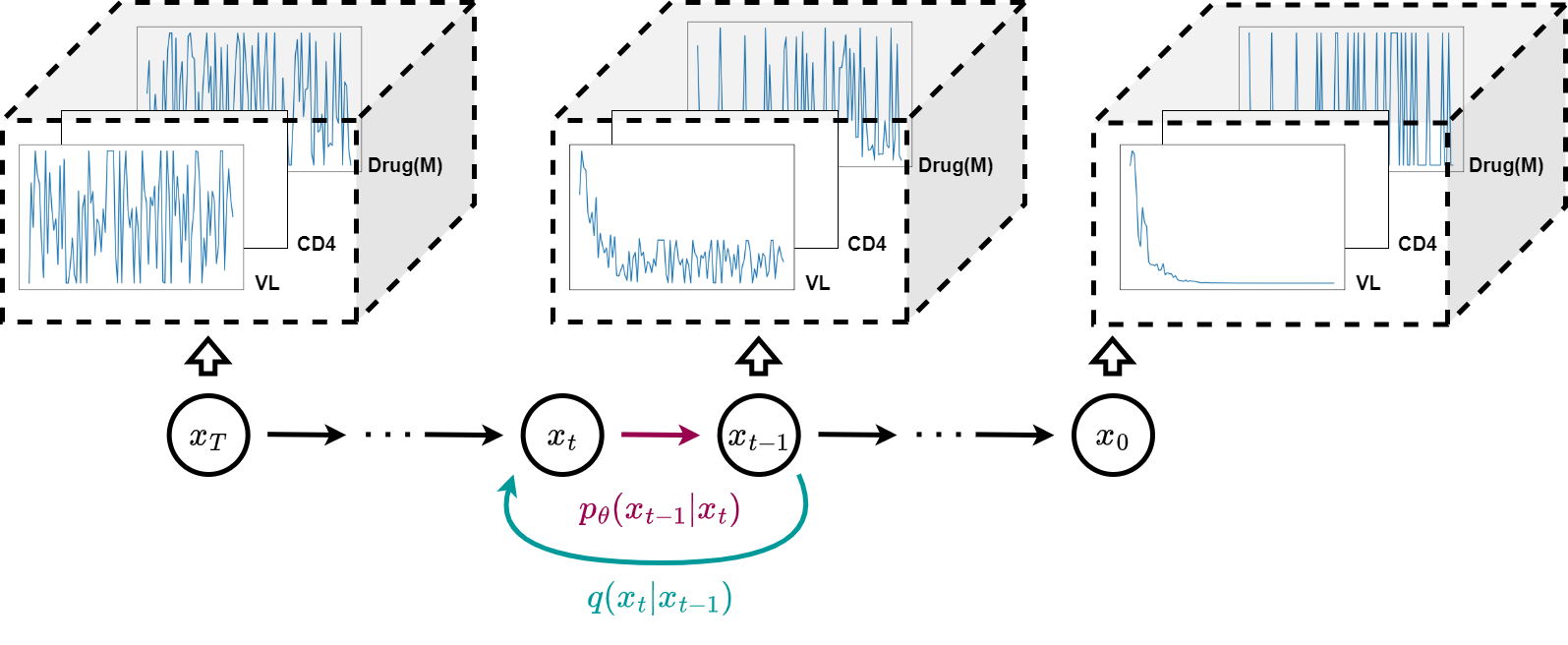
The DPM framework consists a forward diffusion process (in cyan) and a reverse diffusion process (in magenta) to process sequential data . The goal is to denoise the data at each timestep iteratively, resulting in a set of clean and novel time-series variables. Refer to Section 3 for details on the DPM.
Generative Adversarial Networks (GANs) (Goodfellow et al., 2014; Arjovsky et al., 2017; Gulrajani et al., 2017) have proven to be effective generative models, with applications found on images (Yu et al., 2018), texts (Xu et al., 2018), and audios (Pascual et al., 2017). However, training GAN-based models is notoriously difficult because they suffer from unstable training (Thanh-Tung et al., 2019) and mode collapse (Goodfellow, 2016). The former decreases the quality of the synthetic data and the latter reduces diversity. Both phenomena cause GANs to generate ill-represented patient states; and this would negatively impact the utility of the synthetic dataset, causing downstream machine learning models to learn biases that may inflict patient harm (Challen et al., 2019).
Lately, the diffusion probabilistic models (DPMs) (Sohl-Dickstein et al., 2015; Ho et al., 2020) shown in Figure 1 are emerging as one of the top alternative generative frameworks. Similar to GANs, DPMs are extensively applied in images (Dhariwal & Nichol, 2021), texts (Austin et al., 2021), and audios (Kong et al., 2020). In addition, Ramesh et al. (2022) demonstrated that their model (i.e., DELL-E2) could generate highly flexible and creative images with DPMs from text prompts. Using the Fréchet inception distance (FID) (Heusel et al., 2017), Ramesh et al. further demonstrated that DPMs achieved higher realism than various GAN-based models. Dhariwal & Nichol (2021) reported similar findings that DPMs beat GANs on image synthesis.
More recently, DPMs are starting to find applications for electronic health records (EHRs). In a study conducted by Zheng & Charoenphakdee (2022), the authors demonstrated that DPMs can be utilised for the imputation of missing values in clinical tabular data. However to support the developmet of RL, DPMs would need to overcome unique challenges to generate synthetic time-series data over mixed-type variables. To address this, we propose a novel DPM (see Section 5) that is capable of effectively generating time-series clinical datasets for acute hypotension, sepsis, and the antiretroviral therapy for human immunodeficiency virus (ART for HIV) (see Section 4). This constitutes a technical contribution to the field.
In this study, we aim to produce synthetic datasets that can be publicly distributed to hasten research in machine learning. This work marks the first use of DPM to generate synthetic longitudinal EHRs that capture mixed-type variables. As such, a crucial component of our work involves investigating the advantages and caveats of utilising DPMs for this purpose. To assess the validity of our simulated datasets, we conducted three distinct evaluations: (1) a comparison of the statistical properties of synthetic variables with real data (refer to Sections 6.2.1 – 6.2.3); (2) a comparison of the utility (Rankin et al., 2020) of the datasets for developing RL agents (refer to Section 6.2.5); and (3) an estimation of the patient disclosure risk (El Emam et al., 2020) (refer to Section 6.2.4).111To facilitate future research, our code and synthetic dataset will be made available after the paper is published. Follow our research progress on https://healthgym.ai/.
2 Related Work
This section discusses training difficulties in GANs and some existing clinical applications of GANs.
2.1 The Difficulty of Fine-tuning GANs
GANs consist of two sub-networks – a generator and a discriminator222WGAN (Arjovsky et al., 2017) replaces the discriminator with a critic to rate the realisticness of all inputs.. These sub-networks participate in a two-player minimax game where the goal is to find a Nash equilibrium (Goodfellow et al., 2014). The generator creates synthetic data from a random latent prior, while the discriminator aims to determine the authenticity of the generated data by comparing it to real data. Ideally, when the discriminator has optimised and the difference between real and generated data is minimized, the generator has learned to model the underlying probability distribution of the real data.
The training of GANs interleaves the updates of the two sub-networks. This interplay can result in instability in the training process (Kodali et al., 2017; Mescheder et al., 2018), which causes fluctuations in the loss over time (Thanh-Tung et al., 2019), as well as mode collapse (Goodfellow, 2016), where the generator outputs the same sample repeatedly, reducing diversity in the generated data. To mitigate these challenges, prior studies have proposed several implementations to improve the stability and convergence of GAN training, including modifications to the network architecture (Radford et al., 2015), learning objectives (Arjovsky et al., 2017; Gulrajani et al., 2017), and auxiliary experimental setups (Salimans et al., 2016; Sønderby et al., 2016). Additionally, researchers have proposed techniques to mitigate mode collapse by measuring the diversity of the generated data through features learned within the GAN sub-networks. This has been achieved through methods such as minibatch discrimination (Salimans et al., 2016) and moment matching (Li et al., 2017).
There are also many theoretical work on GANs that emphasises the optimality on the minima (Nagarajan & Kolter, 2017; Mescheder et al., 2017; 2018) as well as the convexity of the learning objectives (Kodali et al., 2017). One approach enforces Lipschitz constraints on the discriminator network (Gulrajani et al., 2017; Liu et al., 2019); and another line of research has focused on improving the design of the discriminator or using multiple discriminators (Srivastava et al., 2017; Mordido et al., 2020; Thanh-Tung & Tran, 2020) to reduce the risk of catastrophic forgetting (McCloskey & Cohen, 1989; Kuo et al., 2021) – the abrupt lost of learnt knowledge by repetitive incremental update – in the discriminator to mitigate mode collapse.
2.2 GANs in the Healthcare Domain
While GANs have made significant advancements over the years, they still face certain limitations in the medical domain. Despite extensive research, GANs have primarily been limited to synthesising one type of data. For example, Choi et al. (2017) (i.e., MedGAN), Xie et al. (2018), and Camino et al. (2018) only support the generation of discrete variables; while Beaulieu-Jones et al. (2019) only support numeric variable simulations. Despite recent progress, GAN-generated datasets are largely static in nature (Park et al., 2018; Lu et al., 2019; Yoon et al., 2020; Walia et al., 2020) and may only be suitable for developing predictive algorithms. There is a scarcity of literature on GAN-generated datasets suitable for RL agents (Li et al., 2021; Kuo et al., 2022b), and hence there remains a need for further research in this area to address these limitations.
MedGAN (Choi et al., 2017) has gained popularity in clinical research and is frequently used as a baseline model (Baowaly et al., 2019a; b; Torfi & Fox, 2020). Despite its popularity, a study by Goncalves et al. (2020) found that MedGAN failed to accurately represent multivariate categorical medical data as it performed unfavourably on the log-cluster (Woo et al., 2009) metric.
Similarly, the Health Gym GAN (Kuo et al., 2022b), capable of generating mixed-type time-series clinical data, was found to be susceptible to mode collapse. In an extended study by the same panel of authors (Kuo et al., 2022a), they found that mode collapse negatively impacted the utility of the synthetic dataset because patients of minority ethnicity could be neglected during the synthesis procedure. To mitigate this issue, the authors stored features from the real data in an external buffer during training and replay them to the generator during synthesis. Marchesi et al. (2022) also found that by using a conditional architecture, the Health Gym GAN could synthesise data that captured a higher level of detail in the real data feature space.
In conclusion, applications of GANs in the medical domain are limited by mode collapse and training instability. Moreover, Kuo et al. (2022a) reported that previous solutions for preventing mode collapse in computer vision (Larsen et al., 2016; Salimans et al., 2016; Li et al., 2017; Mangalam & Garg, 2021) prove ineffective for mixed-type time-series clinical data. As an alternative, DPMs may circumvent these limitations, as they are not known for mode collapse and training instability.
3 Diffusion Probabilistic Models
DPMs approximate real data distributions using two main processes: a forward
diffusion process and a reverse diffusion process. Our work mainly concerns the frameworks of Sohl-Dickstein et al. (2015) and Ho et al. (2020); and see more work based on the principle of diffusion in Song et al. (2021a) and Nichol & Dhariwal (2021).
3.1 The Framework
The forward diffusion process adds Gaussian noise to a sample from in time-steps,
| (1) |
where the magnitude of the noise is controlled by a pre-defined variance schedule . This results in a gradual loss of distinguishable features in the sample as increases. Furthermore, using properties of the Gaussian distribution, we can rewrite
| (2) |
where and .
Then, a reverse diffusion process removes noises to synthesise a data as if it were sampled from the real data distribution . A model with weights is learned to approximate the conditional probabilities (via mean and covariance ) between and the Gaussian noise input
| (3) |
3.2 Sampling and Training
The forward process is tractable when conditioned on :
| (4) | |||
| (5) |
and Ho et al. (2020) showed a DPM should learn to configure
| (6) |
to predict the added noise in at time in Equation (1) via approximating .
The perturbed inputs from Equation (2) can be rewritten as
| (7) |
Combined with the in Equation (6), Ho et al. (2020) further showed that optimising
| (8) |
is equivalent333 The equivalent loss is actually with the additional coefficients. However Ho et al. (2020) noted that it was beneficial to train without the additional coefficients. to optimising the negative log-likelihood using the variational lower bound.
4 Ground Truth Datasets
We based our work on the Health Gym project (Kuo et al., 2022b), which used GANs to generate synthetic longitudinal data from two health-related databases: MIMIC-III (Johnson et al., 2016) and EuResist (Zazzi et al., 2012). The authors used these databases to generate synthetic datasets for the management of acute hypotension and human immunodeficiency virus (ART for HIV). The patient cohorts were defined using inclusion and exclusion criteria from previous studies: Gottesman et al. (2019) for acute hypotension and Parbhoo et al. (2017) for ART for HIV. The generated datasets include a comprehensive set of variables that can be utilised as observations, actions, and rewards in RL problems aimed at managing patient illnesses. See all variables in Appendix A.
Acute Hypotension
This dataset was extracted from MIMIC-III and was originally proposed by Gottesman et al. (2019). It comprises of 3,910 patients with 48-hour clinical variables, aggregated per hour in the time-series. The dataset includes variables with suffix (M) to indicate the measurement at a specific point in time and is significant due to its informativeness in missing data in clinical time series, which can indicate the need for laboratory tests. In their work, Gottesman et al. utilised this dataset to develop an RL agent that suggested optimal fluid boluses and vasopressors for acute hypotension management, with actions being made in a discrete action space by binning the boluses and vasopressors into multiple categories. Refer to Table 2 for more details.
ART for HIV
The real HIV dataset is based on a cohort of individuals from the EuResist database, as proposed by Parbhoo et al. (2017). The study employs a mixture-of-experts approach for therapy selection, utilising kernel-based methods to identify clusters of similar individuals and an RL agent to optimise treatment strategy. The dataset consists of 8,916 individuals who started therapy after 2015 and were treated with the 50 most common medication combinations, including 21 different types of medications. Demographics, viral load (VL), CD4 counts, and regimen information are included in the dataset. The length of therapy in the dataset varies, thus the records were truncated and modified to the closest multiples of 10-month periods, resulting in a shortest record length of 10 months and a longest record length of 100 months, each summarising patient observations over a 1-month time period. Again, we include binary variables with the suffix (M) to indicate whether a variable was measured at a specific time. Refer to Table 3 for more details.
5 Methods
This section details the setups for generating mixed-type time-series data with DPMs.
5.1 Data Formulation for Mixed-Type Inputs & Outputs
For each iteration, we draw ground truth data from the set of clinical datasets (see Section 4), and reformulate it to (to be addressed below). We also select a noise level and its corresponding strength of perturbation to introduce corruption to following Equation (2) to acquire the noisy inputs . To estimate the manually injected noise of Equation (7), we feed into a tailored implementation of U-Net (Ronneberger et al., 2015), which serves as our backbone network for the denoising operations. The output of the U-Net network is the predicted estimation for .
Our datasets encompass numeric, binary, and categorical variables. Hence, we elaborate on the data formulation prior to presenting it to the model. The ground truth data is partitioned as
, with the numeric subset and the non-numeric subset . We transform each numeric feature in to the range and derive . Each non-numeric variable is converted into a list of one-hot vectors where the observed class is assigned a value of 1 and the others a value of 0. Here are some examples:
-
•
For the binary variable Gender = Female, we have
, and -
•
for the categorical variable Ethnicity = African, we have
.
We denote the aggregate of all one-hot vectors as ; and that
. Embeddings (Landauer et al., 1998; Mikolov et al., 2013; Mottini et al., 2018) are not necessary in our framework. The forward diffusion process of the DPM (refer to Equation (7)) directly applies noise to the one-hot vectors.
At test time, we randomly sample a noisy input from a Gaussian distribution. Then, we iteratively estimate the corruption at step using our U-Net backbone to generate a less noisy as per Equation (9). Once444Similar to Ho et al. (2020), we used and for both the clean inputs and the denoised, reconstructed output; the terms should thus be used in context of before and after the reverse diffusion process. we reach the allegedly clean and novel data , we compartmentalise it into and to reverse the transformation in , resulting in . Next, we employ softmax to recover the non-numeric variables such that .
The dimensionality of the noisy input is , where corresponds to the batch size, denotes the length of the time-series, and that there is 1 feature channel for all the variables. In Section 4, it was mentioned that all acute hypotension data possess a fixed sequence with a length of 48 units, hence . On the other hand, the HIV data has variable lengths and we utilise zero-padding to bring all the data to a pre-defined maximal length of . This setup hence obviates the need for curriculum learning (Bengio et al., 2009) to enable training.
Moreover, inferring the size is a straightforward task, as it solely involves concatenating the numeric and one-hot representations of the binary and categorical variables in . To illustrate, consider the ART for HIV dataset, whose variable specifications are provided in Table 3. By summing up the corresponding levels of every variable (with 1 for numeric variables), we obtain that
.
Likewise, we deduce that as per its respective specifications in Table 2.

Our U-Net is depicted in the top left panel, with the down-sampling, bottleneck, and up-sampling procedures denoted by the colors red, purple, and blue, respectively. Top right: The presence of linear transformations for pre- and post-processing (see Section 5.2.1-d)). Bottom right: The local features in each resolution level is processed with block processing units and linear transformations (see Section 5.2.1-d)). Bottom left: the anatomy shared by all blocks (see Section 5.2.1-c)).
5.2 The U-Net Backbone
U-Net (Ronneberger et al., 2015) is a convolutional neural network (CNN) architecture originally developed for medical image segmentation. As shown in Figure 2, the architecture has many details. The down-sampling (Zeiler & Fergus, 2014) compartment extracts high-level features from noisy data, while skip connections (Venables & Ripley, 2013) maintain fine-grained details and spatial information. The up-sampling compartment estimates noise for reconstructing clean data, leveraging localised features via the skip connections. U-Net is especially useful in denoising spatially correlated noise of varying intensities; and has been employed in various DPM applications (Saharia et al., 2022; Ho et al., 2022; Li et al., 2022).
5.2.1 The Modules
We depicted the U-Net processing procedure in Figure 2. Refer to hyper-parameters in Section 6 and examples of the dimensionality change in intermediate neural activations in Section 6.1.
5.2.1-a): Embedding the noise level
In Equation (6), the noise prediction process of DPM is enabled via to create to predict noise . Notably, is informed by noise level , which is used to iteratively estimate noise across various levels. To this end, we adopt the Transformer sinusoidal position embedding method (Vaswani et al., 2017), as applied in Ho et al. (2020), to featurise the noise level. These noise level embeddings are then incorporated into the U-Net architecture, and are fed as input to each intermediate neural activation stage that arises from the down- and up-sampling operations.
5.2.1-b): Down- and up-sampling
All CNNs employed in our design are one-dimensional (1-D) and do not possess a causal architecture. Thus when we denoise the noisy acute hypotension datum (see Section 5.1) with a fixed length of , the U-Net could simultaneously denoise the noisy data at positions 10 and 20. Our U-Net hence processes data similar to the autoencoding style of BERT (Devlin et al., 2019), as opposed to the autoregressive style of GPT (Radford et al., 2018) (i.e., we are not limited to denoising from left-to-right in a single direction). See more discussion in Section 5.2.1-d).
5.2.1-c): Block feature extractor
After each stage of sampling operation, the noisy data is further processed while maintaining the same resolution level. Within each level, we utilise three successive feature extraction blocks, each composed of layer normalisation (Ba et al., 2016) followed by two 1-D CNNs.
5.2.1-d): Distinctive Additions to Our U-Net Architecture
We found that the application of the 1-D CNNs alone is insufficient for denoising. As elaborated upon in Section 5.2.1-b), 1-D CNNs have the capability to denoise the noisy data simultaneously at positions 10 and 20, but for each feature independently. For ART for HIV, denoising VL is hence done independently of the regimen taken. While 2-D CNNs may seem more viable, an incorrect kernel size can still cause the erroneously denoising the of {VL, regimen} (in the kernel), while leaving out the relevant information of {CD4, Ethnicity} (out of the kernel). The need to concurrently denoise multiple time-series variables introduces a level of complexity that is not encountered in the DPM’s application in speech (Lu et al., 2022).
This can be addressed by applying additional linear transformation layers on the dimension of . As a consequence, the U-Net no longer denoises data at a variable level and instead denoises data on their latent features. Inspired by Lin et al. (2013), we also include linear transformations to each up- and down-sampling 1-D CNN (see the bottom right panel of Figure 2) to process local patches within the receptive field.
Additional linear transformations are then employed on the final up-sampling output. This restructures the predicted noise made on the latent structure back to the sequences on .
5.3 Auxiliary Loss Functions
Capturing both individual variable fidelity and correlations is crucial for realistic synthetic EHR. Previous studies in GANs used auxiliary loss functions, such as separate encoders and matching loss (Li et al., 2021), or assessed real data correlation before training (Kuo et al., 2022b). However, these approaches synthesise data per iteration, making them computationally costly. Including such losses in DPM is prohibitively expensive due to DPM’s slow sampling nature (Xiao et al., 2022).
To circumvent the iterative denoising in Equation (9), we estimate a one-step reconstruction loss
| (10) | |||
| (11) |
We utilise the predicted noise from the U-Net to replace the actual noise , and apply a one-step reverse process to approximate the clean data using . This is analogous to taking a large step on the vector field (Song & Ermon, 2019; Song et al., 2021b), and may result in overshooting during the reconstruction dynamics. Hence, the use of is restricted solely to our auxiliary loss.
We introduce a second auxiliary loss function to our model, defined as
| (12) | |||
| (13) |
At each iteration, we construct two random matrices and that do not require training. These matrices are used to project the clean data and its reconstructed counterpart to a latent space, and the difference between them is minimised. This approach is inspired by Salimans et al. (2016)’s mini-batch discrimination technique and aims to minimise the variability of the variable combinations in a randomly projected feature space.
6 Experimental Setup
This section details the hyper-parameters implemented in our experiments and the performance metrics utilised to evaluate the quality of our generated dataset. Our evaluation involved comparing our synthetic dataset with the datasets presented in Kuo et al. (2022b). The lack of baseline models can be attributed to the limited amount of literature addressing the generation of longitudinal clinical datasets that possess mixed-type variables. Additionally, only the synthetic datasets provided by Kuo et al. (2022b) were made publicly available for conducting comparisons.
Henceforth, in this manuscript, we employ the following notation:
to denote the ground truth dataset;
to refer to the synthetic dataset generated via Kuo et al. (2022b)’s GAN; and
to represent the alternative synthetic dataset generated using our DPM setup.
6.1 Hyper-parameters
Hyper-parameters for the U-Net
Following Section 5.2.1-d), we choose to linearly project the variables in the input to a latent space of dimensionality 256. After this preliminary step, we employ our U-Net for denoising.
As detailed in Section 5.2.1-b), we adopt 3 distinct resolution levels. More specifically, resolution level 1 maintains the initial length of the noisy sequence for all time-series data, whereas the succeeding resolution levels condense the sequences while augmenting feature dimensions. In resolution level 2, all time-series have feature size 10, and in resolution level 3, all time-series possess feature size 20, regardless of the underlying dataset. However, the alteration in the length of the time-series depended on the dataset. For acute hypotension, resolution level 1 sequences span 48 time steps, which are subsequently reduced to 12 and 3 in resolution levels 2 and 3, respectively. Likewise in ART for HIV, they change from length 100 to 10 and then 3.
Following the previous descriptions, the 1-D CNNs employed in the blocks of Section 5.2.1-c) possess feature dimensions of 10 and 20 at resolution levels 1 and 2 respectively. Whereas the features in the bottleneck of resolution level 3 reduces from 20 to 10, subsequently reverting to 20.
An example using acute hypotension
The input data comprises a sequence length of 48 and variables of 37 (see Section 5.1). We project and contruct the latent structure of the noisy data in . In the subsequent use of U-Net, the dimensionality transforms to in resolution level 2 and then in resolution level 3.
Hyper-parameters for the DPM & Optimisation
We set the maximum perturbation at and the minimum at (see Equation (1)) across both datasets. However, we use for acute hypotension and for ART for HIV. The intermediate perturbations are distributed uniformly across the levels. As previously stated in Section 5.2.1-a), the denoising procedure of our DPM is informed by the noise level . This information is conveyed to the U-Net architecture as a Transformer sinusoidal position embedding, featuring an embedding dimensionality of .
Our DPMs are updated using the Adam optimiser (Kingma & Ba, 2014) with learning rate . We employ a batch size of for the acute hypotension and ART for HIV. The DPMs are trained for epochs for acute hypotension and epochs for ART for HIV. In addition, the losses are weighted at a ratio of for , , and (see Section 5.3), respectively.
6.2 Metrics
We put forth five desiderata:
-
•
Section 6.2.1: that all generated variables to exhibit individual realism;
-
•
Section 6.2.2: that the collective realism of all variables hold across time;
-
•
Section 6.2.3: that there exists a sufficiently high level of diversity in variables;
-
•
Section 6.2.4: that our synthetic datasets ensure patient privacy; and
-
•
Section 6.2.5: that our datasets can function as a substitute for a genuine dataset in
downstream model construction.
6.2.1 Assessing Individual Realisticness
We leverage two plots to assess the individual realisticness. For numeric variables, we use kernel density estimations (KDEs) (Davis et al., 2011) to overlay the synthetic distribution on top its genuine counterpart. For binary and categorical variables, we use side-by-side barplots to demonstrate the percentage share of each level.

The sequence of the hypothesis tests.
Following Kuo et al. (2022b) and Hernadez et al. (2023), we perform four statistical tests on the synthetic datasets shown in Figure 3. We begin with the two-sample Kolmogorov-Smirnov (KS) test (Hodges, 1958) to evaluate whether the synthetic variables effectively capture the distributional characteristics of their real counterparts. If a synthetic variable passes the KS test, it is deemed to be realistic and can be considered as having been drawn from the real datasets. Otherwise, we seek to identify the underlying reasons for its lack of realism.
The perceived lack of realism could be understood using the Student’s t-test (Yuen, 1974) and the F-test. Snedecor’s F-test (Snedecor & Cochran, 1989) is used for numeric variables; and we use the analysis of variance F-test for binary and categorical variables. The t-test verifies the alignment between means, while the F-test assesses the agreement in variances. However, in the event that a synthetic variable fails the KS test, neither the t-test nor the F-test can be used to assess the reliability of the synthetic variable. Hence, we choose the three sigma rule test (Pukelsheim, 1994) (by default, with 2 standard deviations) to evaluate whether the synthetic values fall within a plausible range of real variable values.
In contrast to image generation, we cannot employ the inception score (IS) (Salimans et al., 2016) and the Fréchet inception distance (FID) (Heusel et al., 2017) to evaluate the quality of our generated data. These metrics rely on the Inception v3 model (Szegedy et al., 2015), which is unsuitable for analysing our longitudinal EHR data. Therefore, we follow the lead of Goncalves et al. (2020) and add the Kullback-Leibler (KL) divergence as a complementary measure to estimate the similarity between the synthetic and real data distributions for a given variable.
We start with a preparation stage in which we bin each numeric variable into 20 equivalent classes. Then, for each discretised numeric variable, binary variable, and categorical variable, we calculate the KL divergence between the true distribution and the learned distributions
| (14) |
Since KL divergence is defined at the variable level, we apply it to each variable individually on the synthetic datasets and and then determine how many variables have a lower (and hence better) score. While Goncalves et al. (2020) aggregated all their individual KL divergences, their synthetic dataset only contained categorical variables. Therefore, we find it beneficial to compare the KL divergence on a case-by-case basis for our mixed-type variables.
6.2.2 Correlation Analysis
We employ Kendall’s rank correlation (Kendall, 1945) to assess the relationships among variables in the mixed-type datasets. The correlation is computed in two ways: first, we calculate the static correlations among all data points under the classic setup; second, we estimate the average dynamic correlations following the approach of Kuo et al. (2022b).
The dynamic correlation is computed in two stages. Initially, we decompose each variable of every patient into a trend and a cycle using linear deconstruction, as shown below:
| (15) |
Trends reveal macroscopic patterns in the time series data, such as overall increasing or decreasing trends, while cycles help us understand information on the microscopic level, such as periodic behaviours. After detrending the variables, we calculate the correlations separately for the trends and cycles and then average the values across all patients.
6.2.3 Evaluating Diversity on the Data Structure
To assess the level of diversity present in our synthetic datasets, we employ two metrics: the log-cluster metric (Woo et al., 2009) and category coverage (CAT) proposed in Goncalves et al. (2020). The former, formulated as
| (16) |
measures the difference in latent structures between the real and synthetic datasets. To compute , we first sample records from both the real and synthetic datasets and then merge the sub-datasets to perform a cluster analysis via k-means with clusters. Here, represents the total number of records in cluster , while and denote the number of real and synthetic records in cluster , respectively. We repeat this process 20 times for each synthetic dataset, with each repetition involving a sample of 100,000 real and synthetic records. A lower score indicates that the synthetic datasets are more realistic.
The latter metric, CAT, is defined as
| (17) |
where is the total number of binary and categorical variables, and and represent the real and synthetic datasets, respectively, for the -th variable. Specifically, CAT measures the completeness of the non-numeric classes in the synthetic datasets; it is the higher the better.
6.2.4 Security Estimation
We conduct two tests. First, we examine the minimum Euclidean distance between synthetic and actual records and verify that it is greater than zero, thus preventing any real records from being leaked into the synthetic dataset. Then, we utilise the sample-to-population attack in El Emam et al. (2020) to assess the potential risk of an attacker learning new information by linking an individual in the synthetic dataset to the actual dataset.
The sample-to-population attack involves quasi-identifiers, which are variables that may reveal an individual’s identity, such as Gender and Ethnicity for the ART for HIV dataset. Equivalent classes are then formed by combining these variables, resulting in groups such as Male + Asian and Female + African. The risk associated with linking a synthetic patient is estimated with
| (18) |
where represents the total number of records in the synthetic dataset, equals one if the equivalent class of synthetic is present in both datasets, and denotes the cardinality of the equivalent class in the actual dataset.
6.2.5 Utility Investigation
We employ both the synthetic and real datasets to train RL agents, and we consider a synthetic dataset to achieve a high level of utility if an RL agent trained on both real and synthetic datasets generates similar actions when presented with clinical conditions of patients.
We partitioned each dataset into a set of observational variables and a set of action variables. The observational variables describe the clinical condition of a patient, while the action variables define the actions an RL agent could take. We adopt the approach in Liu et al. (2021) to reduce the observational dimensionality to five variables using cross decomposition (Wegelin, 2000). Next, we applied K-Means clustering (Vassilvitskii & Arthur, 2006) with 100 clusters to define the state space and assigned each data point to their corresponding cluster label. The action space was defined as the set of unique values of the action variables.
Subsequently, we employed published reward functions to determine the optimal actions that an RL agent should take given a patient state555Refer to Gottesman et al. (2019) and Parbhoo et al. (2017) for the reward functions for acute hypotension and ART for HIV. In addition, see Sections 7.1 in the Appendix of Kuo et al. (2022b) for additional details on the implementation for acute hypotension; and likewise Section 4.3.5 in Kuo et al. (2022a) for ART for HIV.. We select batch-constrained Q-learning (Fujimoto et al., 2019) for utility investigation, and we update the policies for 100 iterations with a step size of 0.01.
7 Experimental Results
This section presents the results of the five desiderata outlined in Section 6.2.
7.1 On the Individual Realisticness of the Variables
Actute Hypotension
The KDE plots666The kernel density estimation uses Gaussian kernels to estimate the probability density function of a continuous variable. Thus, the KDE function can potentially produce tails beyond the range of the data.
and barplots for the individual variable comparisons are presented in Figure 4. The grey bars represent the real variables from , while the respective pink and blue bars in subplots 4(a) and 4(b) depict the synthetic variables in and , generated using Kuo et al. (2022b)’s Health Gym GAN and our DPM. Overall, the distributions in both subplots are comparable to their real counterparts in . We observed that DPM captured the multi-modal nature of clinical variables better than GAN (e.g., PaO2 and Lactic Acid), but we also found that our DPM generated more instances of less common classes in FiO2.
The synthetic variables in our DPM-generated hypotension dataset are representative of their real counterparts in . The statistics in Table 4 in Appendix B revealed that all variables passed the three sigma rule test and are reliable. Most variables passed the KS test and thus captured detailed information in the real distributions. The minority of variables that failed the KS test still passed the t-test and F-test, demonstrating that both the mean and the variance are captured and only missing the extreme details in the cumulative distribution function.
The KL divergences in Table 6 in Appendix B indicated that most variables simulated by the DPM are on-par with those generated using GAN. Only the KL divergence of FiO2 was much larger in , consistent with the previous finding that our DPM simulated less common classes for FiO2.
ART for HIV
Refer to all results in Appendix B. In Figure 8, we observed that the variable distributions in our DPM-generated capture the features of the real variables more accurately than those in generated using GAN in Kuo et al. (2022b). The statistical tests reported in Table 5 indicated that while all DPM-simulated variables are reliable, only VL failed the KS test. However, VL still passed the three sigma rule test; and that the KL divergences in Table 7 revealed that the quality of DPM-simulated distributions are on-par or superior to those generated using GAN.


The left panels depicts correlations in Kuo et al. (2022b)’s . Whereas the middle and right panels respectively depict the correlations in our and those in the ground truth .
7.2 On the Correlations of the Variables
Acute Hypotension
The correlations for acute hypotension are depicted in Figure 5. All panels on the left correspond to the synthetic dataset generated by Kuo et al. (2022b)’s GAN; the middle panels represent our DPM-simulated dataset ; and all panels on the right correspond to the ground truth dataset . Furthermore, Figure 5(a) shows the static correlations, Figure 5(b) illustrates the dynamic correlations in trends, and Figure 5(c) presents the dynamic correlations in cycles.
Figure 5 indicates that the correlations in our DPM-simulated dataset (located in the middle panels) exhibit a stronger resemblance to their real counterparts (located in the right panels) than those generated by GAN (located in the left panels). This applied to all three types of correlations considered, including static correlations as well as two types of dynamic correlations.
ART for HIV
Refer to all results in Appendix B. The correlations are shown in Figure 9. Both Kuo et al. (2022b)’s and our DPM-simulated capture the ground truth correlations. However, we noted that our dataset exhibits a closer alignment with the real dataset ; while the correlations in tend to be exaggerated for both the static and dynamic correlations.
| Dataset | CAT | ||
|---|---|---|---|
| Acute Hypotension | (Kuo et al., 2022b) | -2.1413 | 98.03% |
| (ours) | -2.4103 | 100.00% | |
| ART for HIV | (Kuo et al., 2022b) | -2.130 | 97.50% |
| (ours) | -3.057 | 100.00% | |
It is the lower the better () for ; and higher the better () for CAT.

We visualise the combination of Gender and Ethnicity. Colours grey, pink, and blue respectively indicate the ground truth , Kuo et al. (2022b)’s , and our .
7.3 On Diversity and Data Structure
We calculated the log-cluster metric () and category coverage (CAT) to quantitatively assess the similarity between the latent structure of synthetic datasets and their real counterparts. The outcomes are summarised in Table 1. The CAT score showed that all combinations of binary and categorical variables are present in our DPM-simulated dataset ; but such is not the case for not all combinations in the GAN-generated dataset produced by Kuo et al. (2022b). Moreover, the scores indicated that the latent structure embedded in our is more realistic than that in .
The metrics in Table 1 can be more effectively contextualised through the qualitative analyses presented in Figure 6. For the patient demographics in the ART for HIV, we combined patient Gender and Ethnicity. The colours grey, pink, and blue correspond to the ground truth dataset , Kuo et al. (2022b)’s , and our , respectively. Note, we conducted this analysis only for ART for HIV because the acute hypotension dataset does not include variables relating patient demographics.
We found that our covers all combinations of demographic features present in the real dataset; whereas this is not the case for Kuo et al. (2022b)’s . This discrepancy suggests that mode collapse (as discussed in Section 2) may be occurring in GANs and that while they can capture information relating distribution and correlation, synthetic data diversity is low and it remains challenging for GANs to accurately represent the complex, multi-faceted nature of clinical EHR data.
7.4 Analysis of Risk Assessment Outcomes
Acute Hypotension
The variables in the hypotension dataset (see Table 2 in Appendix A) are all related to the patient’s bio-physiological states and do not contain any sensitive information that may reveal individuals’ identities. Consequently, we only tested Euclidean distances and did not assess the disclosure risk. We found that records in our DPM-simulated synthetic dataset matched none of those in the real hypotension dataset . The minimum Euclidean distance between any synthetic record and any real record was 2.79 (), indicating that no data was leaked into the synthetic dataset.
ART for HIV
Likewise, the minimum Euclidean distance between any real and synthetic HIV record was 0.09 (), thus no real records was leaked into our synthetic dataset . The HIV variables (see Table 3 in Appendix A) contain the quasi-identifiers of Gender and Ethnicity. We combined these two variables to form distinct equivalence classes (e.g., male Asians and female Caucasians). The risk of a successful synthetic-to-real attack was estimated to be 0.076%. This risk is also much lower than the standard threshold of 9% (see Section 6.2.4), signifying that our synthetic HIV dataset can be released with minimal risk of sensitive information disclosure.
7.5 Validation of Synthetic Dataset Utility
Acute Hypotension
After training RL agents to suggest clinical treatments, we used heatmaps to visualize their action patterns. Each tile on the heatmap represents a unique action and its associated number indicates the frequency of that action as a proportion of all actions taken.
We depicted the action patterns of the RL agents for acute hypotension in Figure 7. The action space is spanned by Vasopressor and Fluid Boluses. Subplot (a) exhibits the actions taken by an RL agent trained on the real dataset ; subplots (b) and (c) respectively display the actions taken by RL agents trained on Kuo et al. (2022b)’s synthetic dataset and our DPM-simulated . The heatmap in subplot (c) shows a better alignment with its counterpart in subplot (a), indicating that the RL agent trained on our suggested actions that were more similar to those suggested by the RL agent trained on .
ART for HIV
Refer to all results in Appendix B. For ART for HIV, we also found that our DPM-simulated dataset for has a higher utility than the GAN-generated by Kuo et al. (2022b). Figure 10 shows that when the action space is spanned by Comp. NNRTI and Base Drug Combo, the RL agent trained on suggested the treatment of (NVP, DRV + FTC + TDF) for 48.97% of all actions. This suggests that the GAN model used to generate experienced mode collapse, thus creating an excessive number of synthetic records with similar attributes in . Conversely, we attribute the higher utility in the DPM-simulated to the higher robustness of DPM against mode collapse.
8 Caveats and Negative Outcomes
In this section, we detail some negative outcomes and caveats of our DPM. While thus far we have demonstrated the model’s ability to generate realistic synthetic datasets with high utility that are safe for public use, we have encountered difficulties in representing numeric variables with extremely long tails. Specifically, in the ART for HIV dataset simulated by our DPM, VL failed the KS test (see Table 5), and this issue could be further compounded when multiple long-tailed numeric variables are present.
To further investigate this issue, we tested our DPM on generating variables for a sepsis dataset based on the work of Parbhoo et al. (2017). Although our DPM was capable of generating a reliable sepsis dataset that passed the three sigma rule test, we observed that almost all of the numeric variables with extremely long tails failed the KS test. Moreover, the synthetic sepsis variables usually failed either one or both the t-test and F-test, indicating that our DPM had the tendency to learn biases towards numeric variables with extremely long tails.
Despite these limitations, we found that the synthetic sepsis dataset generated using our DPM exhibits realistic correlations and high diversity. However, we also observed a low utility of this dataset, where an RL agent trained on our synthetic dataset was unable to capture the suggested actions learned by an RL agent trained on the ground truth dataset. This was especially evident when numeric variables with extremely long tails spanned the action space.
In light of these results, we acknowledge the current limitations of our DPM in generating numeric variables with extremely long tails. However, we are committed to addressing this technical issue and plan to update our manuscript once we have optimised our DPM for the sepsis dataset. Refer to Appendix C for a complete discussion on the synthesising a sepsis dataset using our DPM.


We illustrate the recommended policies of RL agents, trained using various acute hypotension datasets. The RL action space is spanned by Vasopressors and Fluid Boluses.
9 Discussion
This paper presents a novel approach for generating realistic EHR data using DPMs. While recent work on DPMs (Zheng & Charoenphakdee, 2022; Yuan et al., 2023) has shown promise in generating EHR data, these synthetic datasets remain simplistic. Our contribution lies in demonstrating that DPMs can simulate longitudinal EHR data over mixed-type variables, enabling downstream machine learning algorithms to be developed for advanced applications such as RL that require dynamic time-related information. To the best of our knowledge, this represented the first use of DPMs for this purpose.
We evaluated our DPM on three datasets, acute hypotension, ART for HIV, and sepsis, and compared its performance to that of GANs, specifically Kuo et al. (2022b)’s Health Gym GAN. Our results show that our DPM generated more realistic datasets than GANs for the acute hypotension and ART for HIV datasets. Of note, our DPM-simulated variables better represented the multi-modal nature of clinical variables and showed better correlation alignment with the real datasets. Furthermore, the RL agent trained on our DPM-simulated datasets closely mirrored the policy learned by an agent trained on the real dataset, indicating higher utility than GAN-simulated datasets.
However, our experiments on sepsis revealed limitations in representing numeric variables with extremely long tails, leading to biases and low utility in certain applications. Our DPM tended to fail the KS, t-test, and F-test for such variables, highlighting the need for further optimisation.
Data Records
Below, we provide details on the synthetic hypotension dataset and the synthetic HIV dataset, which are hosted on PhysioNet and FigShare, respectively. Both datasets are stored as comma separated value (CSV) files and are accessible through https://healthgym.ai/.
The synthetic hypotension dataset comprises 3,910 synthetic patients and contains 48 data points per patient representing time-series of 48 hours. In total, there are 187,680 records (rows) in the dataset, with 22 variables (columns). The first 20 variables are organised as listed in Table 2, and the remaining two variables contain the synthetic patient IDs and the hour in the time series. The dataset is 26.0 MB in size and is generated to be realistic while being safe for public access.
Similarly, the synthetic HIV dataset contains 8,916 synthetic patients and time-series of 60 months with 60 data points per patient. The dataset comprises 534,960 records (rows) in total, with 15 variables, the first 13 of which are listed in Table 3. As with the hypotension dataset, the synthetic patient IDs and the month in the time series are contained in the remaining two variables. The dataset is 40.5 MB in size and is also generated to be realistic while being safe for public access.
Broader Impact
While our proposed DPM yielded synthetic datasets that are realistic and privacy-preserving, it is important to note that they should not be naïvely considered as substitutes for actual datasets. In particular, there is a potential concern that synthetic data may carry forward existing biases or introduce new ones. To mitigate this issue, it is crucial to carefully select the features and data sources used to train the model and to regularly monitor the output data for biases.
Furthermore, despite observing similar optimal policies when comparing our DPM-simulated synthetic datasets with the ground truth, there is still room for further improvements. This suggests that our DPM model, although effective in capturing the complexities of a longitudinal EHR dataset with mixed-type variables, may require further fine-tuning to fully realise its potential.
References
- Arjovsky et al. (2017) Martin Arjovsky, Soumith Chintala, and Léon Bottou. Wasserstein generative adversarial networks. In the International Conference on Machine Learning, 2017.
- Austin et al. (2021) Jacob Austin, Daniel D Johnson, Jonathan Ho, Daniel Tarlow, and Rianne van den Berg. Structured denoising diffusion models in discrete state-spaces. In the Advances in Neural Information Processing Systems, 2021.
- Ba et al. (2016) Jimmy Lei Ba, Jamie Ryan Kiros, and Geoffrey E Hinton. Layer normalization, 2016. Preprint at https://arxiv.org/abs/1607.06450.
- Baowaly et al. (2019a) Mrinal Kanti Baowaly, Chia-Ching Lin, Chao-Lin Liu, and Kuan-Ta Chen. Synthesizing electronic health records using improved generative adversarial networks. Journal of the American Medical Informatics Association, 26(3):228–241, 2019a.
- Baowaly et al. (2019b) Mrinal Kanti Baowaly, Chao-Lin Liu, and Kuan-Ta Chen. Realistic data synthesis using enhanced generative adversarial networks. In the IEEE International Conference on Artificial Intelligence and Knowledge Engineering, 2019b.
- Beaulieu-Jones et al. (2019) Brett K Beaulieu-Jones, Zhiwei Steven Wu, Chris Williams, Ran Lee, Sanjeev P Bhavnani, James Brian Byrd, and Casey S Greene. Privacy-preserving generative deep neural networks support clinical data sharing. Circulation: Cardiovascular Quality and Outcomes, 12(7):e005122, 2019.
- Bengio et al. (2009) Yoshua Bengio, Jérôme Louradour, Ronan Collobert, and Jason Weston. Curriculum learning. In the International Conference on Machine Learning, 2009.
- Bentzen et al. (2021) Heidi Beate Bentzen, Rosa Castro, Robin Fears, George Griffin, Volker Ter Meulen, and Giske Ursin. Remove obstacles to sharing health data with researchers outside of the european union. Nature Medicine, 27(8):1329–1333, 2021.
- Camino et al. (2018) Ramiro Camino, Christian Hammerschmidt, and Radu State. Generating multi-categorical samples with generative adversarial networks. In the ICML Workshop on Theoretical Foundations and Applications of Deep Generative Models, 2018.
- Challen et al. (2019) Robert Challen, Joshua Denny, Martin Pitt, Luke Gompels, Tom Edwards, and Krasimira Tsaneva-Atanasova. Artificial intelligence, bias, and clinical safety. BMJ Quality & Safety, 28:231–237, 2019.
- Choi et al. (2017) Edward Choi, Siddharth Biswal, Bradley Malin, Jon Duke, Walter F Stewart, and Jimeng Sun. Generating multi-label discrete patient records using generative adversarial networks. In the Machine Learning for Healthcare Conference, 2017.
- Davis et al. (2011) Richard A Davis, Keh-Shin Lii, and Dimitris N Politis. Remarks on some nonparametric estimates of a density function. In Selected Works of Murray Rosenblatt, pp. 95–100, 2011.
- Devlin et al. (2019) Jacob Devlin, Ming-Wei Chang, Kenton Lee, and Kristina Toutanova. Bert: Pre-training of deep bidirectional transformers for language understanding. In the Conference of the North American Chapter of the Association for Computational Linguistics, 2019.
- Dhariwal & Nichol (2021) Prafulla Dhariwal and Alexander Nichol. Diffusion models beat gans on image synthesis. In the Advances in Neural Information Processing Systems, 2021.
- El Emam et al. (2020) Khaled El Emam, Lucy Mosquera, and Jason Bass. Evaluating identity disclosure risk in fully synthetic health data: Model development and validation. Journal of Medical Internet Research, 22:23139, 2020.
- Fujimoto et al. (2019) Scott Fujimoto, David Meger, and Doina Precup. Off-policy deep reinforcement learning without exploration. In the International Conference on Machine Learning, 2019.
- Goncalves et al. (2020) Andre Goncalves, Priyadip Ray, Braden Soper, Jennifer Stevens, Linda Coyle, and Ana Paula Sales. Generation and evaluation of synthetic patient data. BMC Medical Research Methodology, 20:1–40, 2020.
- Goodfellow (2016) Ian Goodfellow. NeurIPS 2016 Tutorial: Generative Adversarial Networks, 2016. Preprint at https://arxiv.org/abs/1701.00160.
- Goodfellow et al. (2014) Ian Goodfellow, Jean Pouget-Abadie, Mehdi Mirza, Bing Xu, David Warde-Farley, Sherjil Ozair, Aaron Courville, and Yoshua Bengio. Generative adversarial nets. In the Advances in Neural Information Processing Systems, 2014.
- Gottesman et al. (2019) Omer Gottesman, Fredrik Johansson, Matthieu Komorowski, Aldo Faisal, David Sontag, Finale Doshi-Velez, and Leo Anthony Celi. Guidelines for reinforcement learning in healthcare. Nature Medicine, 25:16–18, 2019.
- Gulrajani et al. (2017) Ishaan Gulrajani, Faruk Ahmed, Martin Arjovsky, Vincent Dumoulin, and Aaron C Courville. Improved training of wasserstein gans. In I. Guyon, U. V. Luxburg, S. Bengio, H. Wallach, R. Fergus, S. Vishwanathan, and R. Garnett (eds.), the Advances in Neural Information Processing Systems, 2017.
- Hernadez et al. (2023) Mikel Hernadez, Gorka Epelde, Ane Alberdi, Rodrigo Cilla, and Debbie Rankin. Synthetic tabular data evaluation in the health domain covering resemblance, utility, and privacy dimensions. Methods of Information in Medicine, 2023.
- Heusel et al. (2017) Martin Heusel, Hubert Ramsauer, Thomas Unterthiner, Bernhard Nessler, and Sepp Hochreiter. Gans trained by a two time-scale update rule converge to a local nash equilibrium. In the Advances in Neural Information Processing Systems, 2017.
- Ho et al. (2020) Jonathan Ho, Ajay Jain, and Pieter Abbeel. Denoising diffusion probabilistic models. In the Advances in Neural Information Processing Systems, 2020.
- Ho et al. (2022) Jonathan Ho, Tim Salimans, Alexey A. Gritsenko, William Chan, Mohammad Norouzi, and David J. Fleet. Video diffusion models. In the ICLR Workshop on Deep Generative Models for Highly Structured Data, 2022.
- Hodges (1958) John L Hodges. The significance probability of the smirnov two-sample test. Arkiv för Matematik, 3(5):469–486, 1958.
- Johnson et al. (2016) Alistair EW Johnson, Tom J Pollard, Lu Shen, H Lehman Li-Wei, Mengling Feng, Mohammad Ghassemi, Benjamin Moody, Peter Szolovits, Leo Anthony Celi, and Roger G Mark. Mimic-iii, a freely accessible critical care database. Scientific Data, 3:1–9, 2016.
- Kendall (1945) Maurice G Kendall. The treatment of ties in ranking problems. Biometrika, 33:239–251, 1945.
- Kingma & Ba (2014) Diederik P Kingma and Jimmy Ba. Adam: A method for stochastic optimization, 2014. Preprint at https://arxiv.org/abs/1412.6980.
- Kodali et al. (2017) Naveen Kodali, Jacob Abernethy, James Hays, and Zsolt Kira. On convergence and stability of gans, 2017. Preprint at https://arxiv.org/abs/1705.07215.
- Komorowski et al. (2018) Matthieu Komorowski, Leo A Celi, Omar Badawi, Anthony C Gordon, and A Aldo Faisal. The artificial intelligence clinician learns optimal treatment strategies for sepsis in intensive care. Nature medicine, 24:1716–1720, 2018.
- Kong et al. (2020) Zhifeng Kong, Wei Ping, Jiaji Huang, Kexin Zhao, and Bryan Catanzaro. Diffwave: A versatile diffusion model for audio synthesis. In the International Conference on Learning Representations, 2020.
- Kuo et al. (2021) Nicholas I Kuo, Mehrtash Harandi, Nicolas Fourrier, Christian Walder, Gabriela Ferraro, and Hanna Suominen. Learning to continually learn rapidly from few and noisy data. In the Meta-Learning and Co-Hosted Competition of the AAAI Conference on Artificial Intelligence, 2021.
- Kuo et al. (2022a) Nicholas I Kuo, Louisa Jorm, Sebastiano Barbieri, et al. Generating synthetic clinical data that capture class imbalanced distributions with generative adversarial networks: Example using antiretroviral therapy for hiv, 2022a. Preprint at https://arxiv.org/abs/2208.08655.
- Kuo et al. (2022b) Nicholas I Kuo, Mark N Polizzotto, Simon Finfer, Federico Garcia, Anders Sönnerborg, Maurizio Zazzi, Michael Böhm, Rolf Kaiser, Louisa Jorm, Sebastiano Barbieri, et al. The health gym: Synthetic health-related datasets for the development of reinforcement learning algorithms. Scientific Data, 9(1):1–24, 2022b.
- Landauer et al. (1998) Thomas K Landauer, Peter W Foltz, and Darrell Laham. An introduction to latent semantic analysis. Discourse Processes, 25:259–284, 1998.
- Larsen et al. (2016) Anders Boesen Lindbo Larsen, Søren Kaae Sønderby, Hugo Larochelle, and Ole Winther. Autoencoding beyond pixels using a learned similarity metric. In the International Conference on Machine Learning, 2016.
- Li et al. (2017) Chun-Liang Li, Wei-Cheng Chang, Yu Cheng, Yiming Yang, and Barnabás Póczos. Mmd gan: Towards deeper understanding of moment matching network. In the Advances in Neural Information Processing Systems, 2017.
- Li et al. (2022) Haoying Li, Yifan Yang, Meng Chang, Shiqi Chen, Huajun Feng, Zhihai Xu, Qi Li, and Yueting Chen. Srdiff: Single image super-resolution with diffusion probabilistic models. Neurocomputing, 479:47–59, 2022.
- Li et al. (2021) Jin Li, Benjamin J Cairns, Jingsong Li, and Tingting Zhu. Generating synthetic mixed-type longitudinal electronic health records for artificial intelligent applications, 2021. Preprint at https://arxiv.org/abs/2112.12047.
- Lin et al. (2013) Min Lin, Qiang Chen, and Shuicheng Yan. Network in network, 2013. Preprint at https://arxiv.org/abs/1312.4400.
- Liu et al. (2019) Kanglin Liu, Wenming Tang, Fei Zhou, and Guoping Qiu. Spectral regularisation for combating mode collapse in gans. In the IEEE International Conference on Computer Vision, 2019.
- Liu et al. (2021) Ran Liu, Joseph L Greenstein, James C Fackler, Jules Bergmann, Melania M Bembea, and Raimond L Winslow. Offline reinforcement learning with uncertainty for treatment strategies in sepsis, 2021. Preprint at https://arxiv.org/abs/2107.04491.
- Lu et al. (2019) Pei-Hsuan Lu, Pang-Chieh Wang, and Chia-Mu Yu. Empirical evaluation on synthetic data generation with generative adversarial network. In the Proceedings of the International Conference on Web Intelligence, Mining and Semantics, 2019.
- Lu et al. (2022) Yen-Ju Lu, Zhong-Qiu Wang, Shinji Watanabe, Alexander Richard, Cheng Yu, and Yu Tsao. Conditional diffusion probabilistic model for speech enhancement. In the IEEE International Conference on Acoustics, Speech and Signal Processing, 2022.
- Mangalam & Garg (2021) Karttikeya Mangalam and Rohin Garg. Overcoming mode collapse with adaptive multi adversarial training, 2021. Preprint at https://arxiv.org/abs/2112.14406.
- Marchesi et al. (2022) Raffaele Marchesi, Nicolo Micheletti, Giuseppe Jurman, and Venet Osmani. Mitigating health data poverty: Generative approaches versus resampling for time-series clinical data, 2022. Preprint at https://arxiv.org/abs/2210.13958.
- McCloskey & Cohen (1989) Michael McCloskey and Neal J Cohen. Catastrophic interference in connectionist networks: The sequential learning problem. In Psychology of Learning and Motivation, 1989.
- Mescheder et al. (2017) Lars Mescheder, Sebastian Nowozin, and Andreas Geiger. The numerics of gans. In the Advances in Neural Information Processing Systems, 2017.
- Mescheder et al. (2018) Lars Mescheder, Andreas Geiger, and Sebastian Nowozin. Which training methods for gans do actually converge? In the International Conference on Machine Learning, 2018.
- Mikolov et al. (2013) Tomas Mikolov, Kai Chen, Greg Corrado, and Jeffrey Dean. Efficient estimation of word representations in vector space, 2013. Preprint at https://arxiv.org/abs/1301.3781.
- Mordido et al. (2020) Gonçalo Mordido, Haojin Yang, and Christoph Meinel. microbatchgan: Stimulating diversity with multi-adversarial discrimination. In the IEEE Winter Conference on Applications of Computer Vision, 2020.
- Mottini et al. (2018) Alejandro Mottini, Alix Lheritier, and Rodrigo Acuna-Agost. Airline passenger name record generation using generative adversarial networks, 2018. Preprint at https://arxiv.org/abs/1807.06657.
- Nagarajan & Kolter (2017) Vaishnavh Nagarajan and J Zico Kolter. Gradient descent gan optimisation is locally stable. In the Advances in Neural Information Processing Systems, 2017.
- Nichol & Dhariwal (2021) Alexander Quinn Nichol and Prafulla Dhariwal. Improved denoising diffusion probabilistic models. In the International Conference on Machine Learning, 2021.
- Nosowsky & Giordano (2006) Rachel Nosowsky and Thomas J Giordano. The health insurance portability and accountability act of 1996 (hipaa) privacy rule: Implications for clinical research. Annual Review of Medicine, 57:575–590, 2006.
- O’Keefe & Connolly (2010) Christine M O’Keefe and Chris J Connolly. Privacy and the use of health data for research. Medical Journal of Australia, 193(9):537–541, 2010.
- Parbhoo et al. (2017) Sonali Parbhoo, Jasmina Bogojeska, Maurizio Zazzi, Volker Roth, and Finale Doshi-Velez. Combining kernel and model based learning for hiv therapy selection. AMIA Joint Summits on Translational Science proceedings, 2017:239, 2017.
- Park et al. (2018) Noseong Park, Mahmoud Mohammadi, Kshitij Gorde, Sushil Jajodia, Hongkyu Park, and Youngmin Kim. Data synthesis based on generative adversarial networks. Proceedings of the VLDB Endowment, 11(10):1071–1083, 2018.
- Pascual et al. (2017) Santiago Pascual, Antonio Bonafonte, and Joan Serrà. Segan: Speech enhancement generative adversarial network. In Interspeech, 2017.
- Prosperi et al. (2010) Mattia CF Prosperi, Michal Rosen-Zvi, André Altmann, Maurizio Zazzi, Simona Di Giambenedetto, Rolf Kaiser, Eugen Schülter, Daniel Struck, Peter Sloot, David A Van De Vijver, et al. Antiretroviral therapy optimisation without genotype resistance testing: A perspective on treatment history based models. PloS one, 5:e13753, 2010.
- Pukelsheim (1994) Friedrich Pukelsheim. The three sigma rule. The American Statistician, 48:88–91, 1994.
- Radford et al. (2015) Alec Radford, Luke Metz, and Soumith Chintala. Unsupervised representation learning with deep convolutional generative adversarial networks, 2015. Preprint at https://arxiv.org/abs/1511.06434.
- Radford et al. (2018) Alec Radford, Karthik Narasimhan, Tim Salimans, and Ilya Sutskever. Improving Language Understanding with Unsupervised Learning. Technical Report, OpenAI, 2018.
- Raghu et al. (2017) Aniruddh Raghu, Matthieu Komorowski, Imran Ahmed, Leo Celi, Peter Szolovits, and Marzyeh Ghassemi. Deep reinforcement learning for sepsis treatment, 2017. Preprint at https://arxiv.org/abs/1711.09602.
- Ramesh et al. (2022) Aditya Ramesh, Prafulla Dhariwal, Alex Nichol, Casey Chu, and Mark Chen. Hierarchical text-conditional image generation with clip latents, 2022. Preprint at https://arxiv.org/abs/2204.06125.
- Rankin et al. (2020) Debbie Rankin, Michaela Black, Raymond Bond, Jonathan Wallace, Maurice Mulvenna, Gorka Epelde, et al. Reliability of supervised machine learning using synthetic data in health care: Model to preserve privacy for data sharing. JMIR Medical Informatics, 8(7):e18910, 2020.
- Ronneberger et al. (2015) Olaf Ronneberger, Philipp Fischer, and Thomas Brox. U-net: Convolutional networks for biomedical image segmentation. In the International Conference on Medical Image Computing and Computer-Assisted Intervention, 2015.
- Saharia et al. (2022) Chitwan Saharia, William Chan, Huiwen Chang, Chris Lee, Jonathan Ho, Tim Salimans, David Fleet, and Mohammad Norouzi. Palette: Image-to-image diffusion models. In the ACM Special Interest Group on Computer Graphics, 2022.
- Salimans et al. (2016) Tim Salimans, Ian Goodfellow, Wojciech Zaremba, Vicki Cheung, Alec Radford, and Xi Chen. Improved techniques for training gans. In the Advances in Neural Information Processing Systems, 2016.
- Snedecor & Cochran (1989) George W Snedecor and Witiiam G Cochran. Statistical methods. Ames: Iowa State University Press, 54:71–82, 1989.
- Sohl-Dickstein et al. (2015) Jascha Sohl-Dickstein, Eric Weiss, Niru Maheswaranathan, and Surya Ganguli. Deep unsupervised learning using nonequilibrium thermodynamics. In the International Conference on Machine Learning, 2015.
- Sønderby et al. (2016) Casper Kaae Sønderby, Jose Caballero, Lucas Theis, Wenzhe Shi, and Ferenc Huszár. Amortised map inference for image super-resolution. In the International Conference on Learning Representations, 2016.
- Song et al. (2021a) Jiaming Song, Chenlin Meng, and Stefano Ermon. Denoising diffusion implicit models. In the International Conference on Learning Representations, 2021a.
- Song & Ermon (2019) Yang Song and Stefano Ermon. Generative modeling by estimating gradients of the data distribution. the Advances in Neural Information Processing Systems, 2019.
- Song et al. (2021b) Yang Song, Jascha Sohl-Dickstein, Diederik P Kingma, Abhishek Kumar, Stefano Ermon, and Ben Poole. Score-based generative modeling through stochastic differential equations. In the International Conference on Learning Representations, 2021b.
- Srivastava et al. (2017) Akash Srivastava, Lazar Valkov, Chris Russell, Michael U Gutmann, and Charles Sutton. Veegan: Reducing mode collapse in gans using implicit variational learning. In the Advances in Neural Information Processing Systems, pp. 3310–3320, 2017.
- Sutton & Barto (2018) Richard S Sutton and Andrew G Barto. Reinforcement Learning: An Introduction. MIT Press, 2018.
- Szegedy et al. (2015) Christian Szegedy, Wei Liu, Yangqing Jia, Pierre Sermanet, Scott Reed, Dragomir Anguelov, Dumitru Erhan, Vincent Vanhoucke, and Andrew Rabinovich. Going deeper with convolutions. In the IEEE Conference on Computer Vision and Pattern Recognition, 2015.
-
European Medicines Agency (2014)
European Medicines Agency.
European medicines agency policy on publication of clinical data for
medical products for human use, 2014.
Access
through http://www.ema.europa.eu/docs/en_GB/document_library/Other
/2014/10/WC500174796.pdf . -
Health Canada (2014)
Health Canada.
Guidance document on public release of clinical information, 2014.
Access through
https://www.canada.ca/en/health-canada/services/drug-health-
product-review-approval/profile-public-release-clinical-
information-guidance/document.html. - Thanh-Tung & Tran (2020) Hoang Thanh-Tung and Truyen Tran. Catastrophic forgetting and mode collapse in gans. In the International Joint Conference on Neural Networks, 2020.
- Thanh-Tung et al. (2019) Hoang Thanh-Tung, Truyen Tran, and Svetha Venkatesh. Improving generalisation and stability of generative adversarial networks. In the International Conference on Learning Representations, 2019.
- Torfi & Fox (2020) Amirsina Torfi and Edward A Fox. Corgan: Correlation-capturing convolutional generative adversarial networks for generating synthetic healthcare records. In the International Flairs Conference, 2020.
- Vassilvitskii & Arthur (2006) Sergei Vassilvitskii and David Arthur. k-means++: The ddvantages of careful seeding. In Proceedings of the ACM-SIAM Symposium on Discrete Algorithms, 2006.
- Vaswani et al. (2017) Ashish Vaswani, Noam Shazeer, Niki Parmar, Jakob Uszkoreit, Llion Jones, Aidan N Gomez, Łukasz Kaiser, and Illia Polosukhin. Attention is all you need. In the Advances in Neural Information Processing Systems, 2017.
- Venables & Ripley (2013) William N Venables and Brian D Ripley. Modern applied statistics with S-PLUS. Springer Science & Business Media, 2013.
- Walia et al. (2020) Manhar Walia, Brendan Tierney, and Susan McKeever. Synthesising tabular data using wasserstein conditional gans with gradient penalty (wcgan-gp). In AICS, 2020.
- Wegelin (2000) Jacob A. Wegelin. A survey of partial least squares (pls) methods, with emphasis on the two-block case. Technical report, University of Washington, 2000.
- Woo et al. (2009) Mi-Ja Woo, Jerome P Reiter, Anna Oganian, and Alan F Karr. Global measures of data utility for microdata masked for disclosure limitation. Journal of Privacy and Confidentiality, 1, 2009.
- Xiao et al. (2022) Zhisheng Xiao, Karsten Kreis, and Arash Vahdat. Tackling the generative learning trilemma with denoising diffusion gans. In the International Conference on Learning Representations, 2022.
- Xie et al. (2018) Liyang Xie, Kaixiang Lin, Shu Wang, Fei Wang, and Jiayu Zhou. Differentially private generative adversarial network, 2018. Preprint at https://arxiv.org/abs/1802.06739.
- Xu et al. (2018) Jingjing Xu, Xuancheng Ren, Junyang Lin, and Xu Sun. Diversity-promoting gan: A cross-entropy based generative adversarial network for diversified text generation. In the Empirical Methods in Natural Language Processing, 2018.
- Yoon et al. (2020) Jinsung Yoon, Lydia N Drumright, and Mihaela Van Der Schaar. Anonymization through data synthesis using generative adversarial networks (ads-gan). IEEE Journal of Biomedical and Health Informatics, 24(8):2378–2388, 2020.
- Yu et al. (2018) Jiahui Yu, Zhe Lin, Jimei Yang, Xiaohui Shen, Xin Lu, and Thomas S Huang. Generative image inpainting with contextual attention. In the IEEE Conference on Computer Vision and Pattern Recognition, 2018.
- Yuan et al. (2023) Hongyi Yuan, Songchi Zhou, and Sheng Yu. Ehrdiff: Exploring realistic ehr synthesis with diffusion models, 2023. Preprint at https://arxiv.org/abs/2303.05656.
- Yuen (1974) Karen K Yuen. The two-sample trimmed t for unequal population variances. Biometrika, 61:165–170, 1974.
- Zazzi et al. (2012) Maurizio Zazzi, Francesca Incardona, Michal Rosen-Zvi, Mattia Prosperi, Thomas Lengauer, Andre Altmann, Anders Sonnerborg, Tamar Lavee, Eugen Schülter, and Rolf Kaiser. Predicting response to antiretroviral treatment by machine learning: The euresist project. Intervirology, 55(2):123–127, 2012.
- Zeiler & Fergus (2014) Matthew D Zeiler and Rob Fergus. Visualizing and understanding convolutional networks. In the European Conference on Computer Vision, 2014.
- Zheng & Charoenphakdee (2022) Shuhan Zheng and Nontawat Charoenphakdee. Diffusion models for missing value imputation in tabular data. In the First Table Representation Workshop of the Advances in Neural Information Processing Systems, 2022.
Author Contributions Statement
Corresponding author: Nicholas I-Hsien Kuo ([email protected])
N.K. and S.B. designed, implemented and validated the deep learning models used to generate the synthetic datasets. L.J. contributed to the design of the study and provided expertise regarding the risk of sensitive information disclosure. Furthermore, N.K. wrote the manuscript and S.B. and N.K. designed the study. All authors contributed to the interpretation of findings and manuscript revisions.
Competing Interests
The authors declare no competing interests.
Acknowledgements
This study benefited from data provided by EuResist Network EIDB; and this project has been funded by a Wellcome Trust Open Research Fund (reference number 219691/Z/19/Z).
Supplementary Materials
Nicholas I-Hsien Kuo, Louisa Jorm, Sebastiano Barbieri
Centre for Big Data Research in Health, the University of New South Wales, Sydney, Australia
*
Corresponding author: Nicholas I-Hsien Kuo ([email protected])
The following appendix provides additional details and supporting information for the paper “Synthetic Health-related Longitudinal Data with Mixed-type Variables Generated using Diffusion Models”. In the main text, we propose a novel method for generating synthetic datasets that capture the mixed-type variables of longitudinal EHRs using DPMs; and we present additional details and extra experimental outcomes in the supplementary materials.
Appendix A Variables of the Datasets
The first dataset, for the management of acute hypotension, contains various clinical variables such as blood pressure and laboratory results. The second dataset, for HIV includes various medication combinations. Complete details and variable lists are provided in Tables 2 and 3.
For data extraction and the inclusion/exclusion criteria, we mainly followed the Supplementary Information provided by Kuo et al. (2022b) in https://www.nature.com/articles/s41597-022-01784-7. Additional guidelines on data formatting can be found in Kuo et al.’s repository https://github.com/Nic5472K/ScientificData2021_HealthGym
Appendix B The Statistical Outcomes
The Statistical Hypothesis Tests
We implemented a series of hierarchical statistical tests as described in Kuo et al. (2022b) to assess the realism of our synthetic variables (see Figure 3). The results of these tests are presented in Tables 4 and 5. Our objective was to determine whether the statistics of those data from the synthetic dataset used to train a neural network would be considered to be highly similar to the real dataset during iterative batch training. To achieve this, we sampled a batch of synthetic and real data with a batch size of for a maximum of iterations (hence the denominators in the Table are ). We then performed the four statistical tests in Figure 3 along the variable dimension. For a full description of the algorithm, please refer to Appendix D.5 on page 44 of Kuo et al. (2022b).
The KL Divergences of the Individual Variables
As mentioned in Section 6.2.1, we used the KL divergence to estimate the similarity between the synthetic and real data distributions for each variable individually. To achieve this, we calculated the KL divergence between the true distribution and the learned distributions according to Equation (14) and presented the full statistics in Tables 6 and 7.
Extra Results on the ART for HIV
To streamline our reporting of results, we have chosen to primarily focus on the findings concerning acute hypotension in the main text. In particular, we have relegated the additional outcomes pertaining to ART for HIV, which largely mirror the successes observed in the acute hypotension study, to the supplementary materials. Refer to the relevant outcomes illustrated in Figures 8 – 10.
| Variable Name | Data Type | Unit | Extra Notes |
|---|---|---|---|
| Mean Arterial Pressure (MAP) | numeric | mmHg | |
| Diastolic Blood Pressure (DBP) | numeric | mmHg | |
| Systolic BP (SBP) | numeric | mmHg | |
| Urine | numeric | mL | |
| Alanine Aminotransferase (ALT) | numeric | IU/L | |
| Aspartate Aminotransferase (AST) | numeric | IU/L | |
| Partial Pressure of Oxygen (PaO2) | numeric | mmHg | |
| Lactate | numeric | mmol/L | |
| Serum Creatinine | numeric | mg/dL | |
| Fluid Boluses | categorical | mL | 4 Classes |
| ; ; | |||
| ; | |||
| Vasopressors | categorical | mcg/kg/min | 4 Classes |
| ; ; | |||
| ; | |||
| Fraction of Inspired Oxygen (FiO2) | categorical | fraction | 10 Classes |
| ; ; | |||
| ; ; | |||
| ; ; | |||
| ; ; | |||
| ; | |||
| Glasgow Coma Scale Score (GCS) | categorical | point | 13 Classes |
| ; ; ; ; | |||
| ; ; ; ; | |||
| ; ; ; | |||
| ; | |||
| Urine Data Measured (Urine (M)) | binary | - - | False; True |
| ALT or AST Data Measured (ALT/AST (M)) | binary | - - | False; True |
| FiO2 (M) | binary | - - | False; True |
| GCS (M) | binary | - - | False; True |
| PaO2 (M) | binary | - - | False; True |
| Lactic Acid (M) | binary | - - | False; True |
| Serum Creatinine (M) | binary | - - | False; True |
This table presents information related to the variables used in the acute hypotension datasets. In addition, we listed the different levels available to the non-numeric variables.
| Variable Name | Data Type | Unit | Extra Notes |
|---|---|---|---|
| Viral Load (VL) | numeric | copies/mL | |
| Absolute Count for CD4 (CD4) | numeric | cells/L | |
| Relative Count for CD4 (Rel CD4) | numeric | cells/L | |
| Gender | binary | - - | Female; Male |
| Ethnicity | categorical | - - | 4 Classes |
| Asian; African; | |||
| Caucasian; Other | |||
| Base Drug Combination | categorical | - - | 6 Classes |
| (Base Drug Combo) | FTC + TDF; 3TC + ABC; | ||
| FTC + TAF; DRV + FTC + TDF; | |||
| FTC + RTVB + TDF; Other | |||
| Complementary INI | categorical | - - | 4 Classes |
| (Comp. INI) | DTG; RAL; | ||
| EVG; Not Applied | |||
| Complementary NNRTI | categorical | - - | 4 Classes |
| (Comp. NNRTI) | NVP; EFV; | ||
| RPV; Not Applied | |||
| Extra PI | categorical | - - | 6 Classes |
| DRV; RTVB; | |||
| LPV; RTV; | |||
| ATV; Not Applied | |||
| Extra pk Enhancer (Extra pk-En) | binary | - - | False; True |
| VL Measured (VL (M)) | binary | - - | False; True |
| CD4 (M) | binary | - - | False; True |
| Drug Recorded (Drug (M)) | binary | - - | False; True |
This table presents information related to the variables used in the ART for HIV datasets. In addition, we listed the different levels available to the non-numeric variables.
| Variable Name | . KS-Test . | . t-Test . | . F-Test . | Three Sigma Rule Test |
|---|---|---|---|---|
| MAP | ||||
| Diastolic BP | ||||
| Systolic BP | ||||
| Urine | ||||
| ALT | ||||
| AST | ||||
| PaO2 | ||||
| Lactic Acid | ||||
| Serum Creatinine | ||||
| Fluid Boluses | - - | - - | ||
| Vasopressors | - - | - - | ||
| FiO2 | - - | - - | ||
| GCS | - - | - - | ||
| Urine (M) | - - | - - | ||
| ALT/AST (M) | - - | - - | ||
| FiO2 (M) | - - | - - | ||
| GCS (M) | - - | - - | ||
| PaO2 (M) | - - | - - | ||
| Lactic Acid (M) | - - | - - | ||
| Serum Creatinine (M) | - - | - - |
| Variable Name | . KS-Test . | . t-Test . | . F-Test . | Three Sigma Rule Test |
|---|---|---|---|---|
| VL | ||||
| CD4 | ||||
| Rel CD4 | ||||
| Gender | - - | - - | ||
| Ethnic | - - | - - | ||
| Base Drug Combo | - - | - - | ||
| Comp. INI | - - | - - | ||
| Comp. NNRTI | - - | - - | ||
| Extra PI | - - | - - | ||
| Extra pk-En | - - | - - | ||
| VL (M) | - - | - - | ||
| CD4 (M) | - - | - - | ||
| Drug (M) | - - | - - |
| Variable Name | KL Divergence from | KL Divergence from (Ours) |
|---|---|---|
| MAP | 0.0724 | 0.0282 |
| Diastolic BP | 0.1837 | 0.0506 |
| Systolic BP | 0.1770 | 0.0374 |
| Fluid Boluses | 0.0014 | 0.1462 |
| Urine | 0.0155 | 0.0337 |
| Vasopressors | 0.0051 | 0.3881 |
| ALT | 0.0196 | 0.0080 |
| AST | 0.0203 | 0.0047 |
| FiO2 | 0.0123 | 0.0846 |
| GCS | 0.0471 | 0.0469 |
| PaO2 | 0.2144 | 0.0929 |
| Lactic Acid | 0.0074 | 0.0842 |
| Serum Creatinine | 0.1270 | 0.0743 |
| Urine (M) | 0.0032 | 0.0076 |
| ALT/AST (M) | 9 | 1 |
| FiO2 (M) | 0.0002 | 0.0068 |
| GCS (M) | 0.0047 | 0.0005 |
| PaO2 (M) | 0.0002 | 0.0016 |
| Lactic Acid (M) | 1 | 0.0004 |
| Serum Creatinine (M) | 0.0005 | 0.0004 |
| Variable Name | KL Divergence from | KL Divergence from (Ours) |
|---|---|---|
| VL | 0.3947 | 0.3482 |
| CD4 | 0.0353 | 0.0318 |
| Rel CD4 | 0.0080 | 0.0088 |
| Gender | 0.2230 | 0.0205 |
| Ethnicity | 0.2047 | 0.0473 |
| Base Combo | 0.1723 | 0.0360 |
| INI | 0.0947 | 0.0926 |
| NNRTI | 0.1921 | 0.1459 |
| extra PI | 0.0597 | 0.0187 |
| VL (M) | 0.0036 | 0.0022 |
| CD4 (M) | 0.0096 | 0.0078 |
| Drug (M) | 0.0001 | 0.0001 |
| pk-En | 0.0324 | 0.0725 |

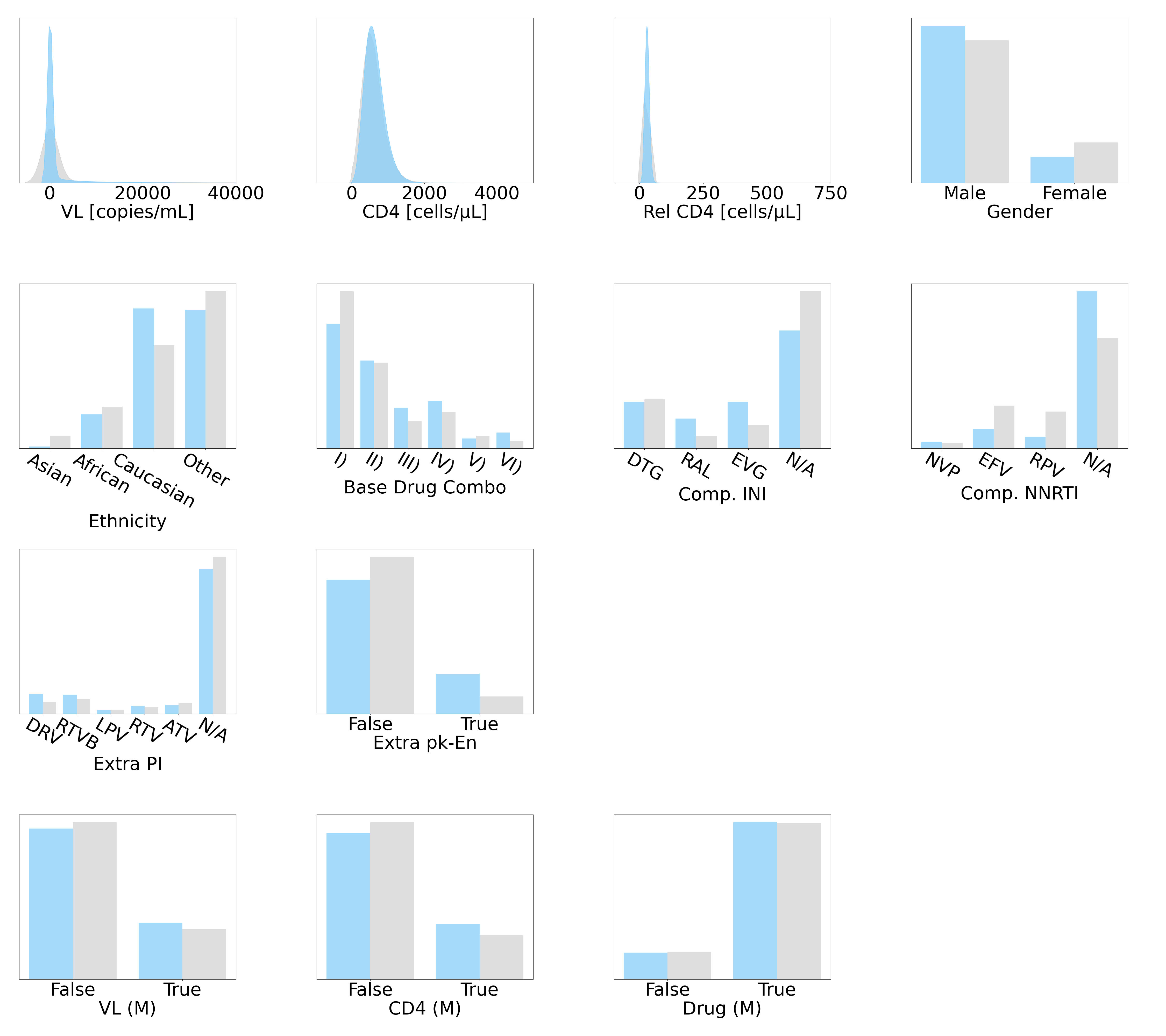


This figure is follows the configuration of Figure 5: the panels on the left, the middle, and the right represents the correlations from the synthetic dataset generated by Kuo et al. (2022b), from our DPM-simulated , and from the ground truth , respectively.


We illustrate the recommended policies of RL agents, trained using various ART for HIV datasets. The RL action space is spanned by Comp. NNRTI and Base Drug Combo.
Appendix C Sepsis
We recognise that our DPM may not be completely fine-tuned or able to represent all EHR variables that exist. To increase transparency and openness in our research, we provide this appendix to outline the unfavorable outcomes of our DPM on a sepsis dataset. Specifically, we detail that their DPM is not yet optimised to represent numeric variables with particularly long tails.
C.1 Background
The real dataset for sepsis management, developed by Komorowski et al. (2018), was extracted from the MIMIC-III database and encompasses 44 variables, including vital signs, laboratory results, mechanical ventilation information, and patient measurements. This dataset is comprised of time-series data for 2,164 patients, with varying durations of hospital stays ranging from 8 to 80 hours, with the data being reported in 4-hour windows, leading to 2 to 20 data points per patient record. The RL agent employed by Komorowski et al. was trained to prescribe doses of intravenous fluids and vasopressors to patients, with rewards assigned based on patients transitioning to a more favorable health state following the actions taken. Refer to Tables 8 and 9 for more details.
C.2 Experimental Setup
The experimental setups used to simulate the sepsis dataset in this study closely follows the descriptions presented in Section 6.1. However, certain modifications were implemented specifically for the sepsis data, which we discuss below.
Given the variable lengths of the sepsis data, zero-padding was utilised to bring all data to a pre-defined maximal length of . Additionally, in line with the reasoning detailed in Section 6.1, we determined . Moreover, the sequence lengths for the sepsis data in the three resolution levels of the U-Net were 20, 5, and 3, respectively.
Training was conducted using a batch size of 32 and we set . The DPMs were trained until convergence, which was achieved after 2000 epochs.
C.3 Individual Realism
The distributions of variables are depicted in Figures 11, 12, and 13. The synthetic variables in from Kuo et al. (2022b) and those in our both effectively capture features of their genuine counterparts in . To quantitatively assess the DPM-generated variables, we conducted statistical tests and present the results in Table 10. The results showed that although all DPM-simulated variables are reliable, a noteworthy fraction of numeric variables (particularly those with significantly elongated tails) failed the KS test, which suggested that DPM may have the potential to encode biases in variable distributions. Notably, the KL divergences in Table 11 revealed that the quality of DPM-simulated distributions is on-par with those generated using Kuo et al. (2022b)’s GAN.
C.4 Correlations
The correlations of synthetic variables generated by Kuo et al. (2022b)’s GAN and our DPM are compared with their real counterparts in Figure 14. Both Kuo et al. (2022b)’s and our DPM-simulated captured the ground truth correlations. Although a minor detail, it could be argued that better represented the dynamic correlations in trends, while better represented the dynamic correlations in cycles.
C.5 Data Diversity
The results presented in Table 12 indicate that the latent structure in our DPM-simulated dataset is comparatively weaker. This finding can be attributed to the observations detailed in Appendix C.3, wherein we identified the presence of numeric variables with extreme long tails in the sepsis dataset. Our DPM struggled to accurately capture the distributional features of such variables, leading to weaker latent structure in the simulated dataset.
Nevertheless, when we examined data diversity in the context of Figure 15, where patient demographics were compared across different cohorts using the Age variable binned into groups of 20-year intervals and combined with patient Gender, we discovered that our DPM-simulated datasets encompassed all possible combinations of demographic features present in the real dataset. This was not the case for Kuo et al. (2022b)’s GAN-generated datasets. Hence, while DPMs may encode bias in numeric variables with extremely long tails, our results demonstrate that DPM-simulated data is better suited for representing cohort diversity.
C.6 Risk Assessment
Using the Euclidean distance test, we discovered that none of the records in our synthetic dataset were identical to any of the records in the real dataset . The smallest distance between the real and synthetic records was 47.00 ().
This dataset also includes the quasi-identifiers of Age and Gender. We combined the Age variable (rounded down to the nearest year) and Gender to create different equivalence classes (e.g., males at 21 years old and females at 37 years old). The risk of a successful synthetic-to-real attack was estimated to be 5.44%. This risk is significantly lower than the suggested threshold of 9%, indicating that releasing our synthetic sepsis dataset carries minimal risk of sensitive information disclosure.
C.7 Utility
However, our experimentation revealed that the utility of our DPM-simulated was unsatisfactory for the sepsis dataset. As depicted in Figure 16, when the action space was spanned by Max Vaso and Input 4H, the RL agent trained on our failed to replicate the actions taken by the RL agent trained on the ground truth . This unfavorable outcome may have resulted from DPM’s learning biases in the distribution of numeric values with extreme long tails, as discussed in Appendix C.3. Although we previously demonstrated that the DPM-simulated sepsis dataset contained reliable variables (see Figure 13), realistic correlations (see Figure 14), and higher diversity in patient demographics (see Figure 6), our still fell short in achieving satisfactory utility.
C.8 Concluding Remark
Our DPM-simulated sepsis dataset did not meet the desired level of utility, and as such, we have chosen not to make it publicly available in its current state. We remain dedicated to addressing this limitation and will continue to explore potential solutions. As new findings emerge, we will update this manuscript to reflect our progress in this area.
| Variable Name | Data Type | Unit | Extra Notes |
|---|---|---|---|
| Age | numeric | year | |
| Heart Rate (HR) | numeric | bpm | |
| Systolic BP | numeric | mmHg | |
| Mean BP | numeric | mmHg | |
| Diastolic BP | numeric | mmHg | |
| Respiratory Rate (RR) | numeric | bpm | |
| Potassium (K+) | numeric | meq/L | |
| Sodium (Na+) | numeric | meq/L | |
| Chloride (Cl-) | numeric | meq/L | |
| Calcium (Ca) | numeric | mg/dL | |
| Ionised Ca++ | numeric | mg/dL | |
| Carbon Dioxide (CO2) | numeric | meq/L | |
| Albumin | numeric | g/dL | |
| Hemoglobin (Hb) | numeric | g/dL | |
| Potential of Hydrogen (pH) | numeric | - - | |
| Arterial Base Excess (BE) | numeric | meq/L | |
| Bicarbonate (HCO3) | numeric | meq/L | |
| FiO2 | numeric | fraction | |
| Glucose | numeric | mg/dL | |
| Blood Urea Nitrogen (BUN) | numeric | mg/dL | |
| Creatinine | numeric | mg/dL | |
| Magnesium (Mg++) | numeric | mg/dL | |
| Serum Glutamic Oxaloacetic Transaminase (SGOT) | numeric | u/L | |
| Serum Glutamic Pyruvic Transaminase (SGPT) | numeric | u/L | |
| Total Bilirubin (Total Bili) | numeric | mg/dL | |
| White Blood Cell Count (WBC) | numeric | E9/L | |
| Platelets Count (Platelets) | numeric | E9/L | |
| PaO2 | numeric | mmHg | |
| Partial Pressure of CO2 (PaCO2) | numeric | mmHg | |
| Lactate | numeric | mmol/L | |
| Total Volume of Intravenous Fluids (Input Total) | numeric | mL | |
| Intravenous Fluids of Each 4-Hour Period (Input 4H) | numeric | mL | |
| Maximum Dose of Vasopressors in 4H (Max Vaso) | numeric | mcg/kg/min | |
| Total Volume of Urine Output (Output Total) | numeric | mL | |
| Urine Output in 4H (Output 4H) | numeric | mL |
This table presents information related to the numeric variables used in the sepsis datasets; to be continued with the binary and categorical variables in Table 9.
| Variable Name | Data Type | Unit | Extra Notes |
|---|---|---|---|
| Gender | binary | - - | Male; Female |
| Readmission of Patient | binary | - - | False; True |
| (Readmission) | |||
| Mechanical Ventilation | binary | - - | False; True |
| (Mech) | |||
| GCS | categorical | point | 13 Classes |
| ; ; ; ; | |||
| ; ; ; ; | |||
| ; ; ; | |||
| ; | |||
| Pulse Oximetry Saturation | categorical | 10 Classes (C) | |
| (SpO2) | C1: ; C2: ; | ||
| C3: ; C4: ; | |||
| C5: ; C6: ; | |||
| C7: ; C8: ; | |||
| C9: ; C10: ; | |||
| Temperature | categorical | Celsius | 10 Classes (C) |
| (Temp) | C1: ; C2: ; | ||
| C3: ; C4: ; | |||
| C5: ; C6: ; | |||
| C7: ; C8: ; | |||
| C9: ; C10: ; | |||
| Partial Thromboplastin Time | categorical | s | 10 Classes (C) |
| (PTT) | C1: ; C2: ; | ||
| C3: ; C4: ; | |||
| C5: ; C6: ; | |||
| C7: ; C8: ; | |||
| C9: ; C10: ; | |||
| Prothrombin Time | categorical | s | 10 Classes (C) |
| (PT) | C1: ; C2: ; | ||
| C3: ; C4: ; | |||
| C5: ; C6: ; | |||
| C7: ; C8: ; | |||
| C9: ; C10: ; | |||
| International Normalised Ratio | categorical | - - | 10 Classes (C) |
| (INR) | C1: ; C2: ; | ||
| C3: ; C4: | |||
| C5: ; C6: ; | |||
| C7: ; C8: ; | |||
| C9: ; C10: ; |
This table presents information related to the binary and categorical variables used in the sepsis dataset. It continues from Table 8; and in addition, we listed the different levels available.


Those from the real datset are in colour grey and variables of the synthetic dataset generated by Kuo et al. (2022b) are in pink.

Those from the real datset are in colour grey and variables of the synthetic dataset generated using our DPM are in blue.
| Variable Name | . KS Test . | . t-Test . | . F-Test . | Three Sigma Rule Test |
|---|---|---|---|---|
| Age | ||||
| HR | ||||
| Systolic BP | ||||
| Mean BP | ||||
| Diastolic BP | ||||
| RR | ||||
| K+ | ||||
| Na+ | ||||
| Cl- | ||||
| Ca++ | ||||
| Ionised Ca++ | ||||
| CO2 | ||||
| Albumin | ||||
| Hb | ||||
| pH | ||||
| BE | ||||
| HCO3 | ||||
| FiO2 | ||||
| Glucose | ||||
| BUN | ||||
| Creatinine | ||||
| Mg++ | ||||
| SGOT | ||||
| SGPT | ||||
| Total Bili | ||||
| WBC | ||||
| Platelets | ||||
| PaO2 | ||||
| PaCO2 | ||||
| Lactate | ||||
| Input Total | ||||
| Input 4H | ||||
| Max Vaso | ||||
| Output Total | ||||
| Output 4H | ||||
| Gender | - - | - - | ||
| Readmission | - - | - - | ||
| Mech | - - | - - | ||
| GCS | - - | - - | ||
| SpO2 | - - | - - | ||
| Temp | - - | - - | ||
| PTT | - - | - - | ||
| PT | - - | - - | ||
| INR | - - | - - |
| Variable Name | KL Divergence from | KL Divergence from (Ours) |
|---|---|---|
| Age | 0.2230 | 0.1945 |
| HR | 0.0171 | 0.0978 |
| Systolic BP | 0.1438 | 0.0689 |
| Mean BP | 0.1520 | 0.0745 |
| Diastolic BP | 0.0179 | 0.1575 |
| RR | 0.0789 | 0.0972 |
| K+ | 0.0293 | 0.1905 |
| Na+ | 0.0737 | 0.0511 |
| Cl- | 0.0618 | 0.1459 |
| Ca++ | 0.1355 | 0.0288 |
| Ionised Ca++ | 0.1040 | 0.1382 |
| CO2 | 0.1776 | 0.0336 |
| Albumin | 0.1259 | 0.0228 |
| Hb | 0.0246 | 0.1049 |
| pH | 0.0186 | 0.0942 |
| BE | 0.0463 | 0.0456 |
| HCO3 | 0.2082 | 0.0840 |
| FiO2 | 0.5679 | 0.7077 |
| Glucose | 0.0179 | 0.0888 |
| BUN | 0.2531 | 0.0675 |
| Creatinine | 0.0213 | 0.0088 |
| Mg++ | 0.0241 | 0.3387 |
| SGOT | 0.0175 | 0.0237 |
| SGPT | 0.0302 | 0.0112 |
| Total Bili | 0.0276 | 0.0670 |
| WBC | 0.0249 | 0.0496 |
| Platelets | 0.1250 | 0.2407 |
| PaO2 | 0.0793 | 0.0618 |
| PaCO2 | 0.0373 | 0.0419 |
| Lactate | 0.0593 | 0.2549 |
| Input Total | 0.0934 | 0.0962 |
| Input 4H | 0.3364 | 0.3682 |
| Max Vaso | 1.9127 | 2.1157 |
| Output Total | 0.1695 | 0.2147 |
| Output 4H | 0.3005 | 0.2988 |
| Gender | 0.0729 | 0.0019 |
| Readmission | 0.0080 | 0.0553 |
| Mech | 0.0108 | 0.0202 |
| GCS | 0.0879 | 0.0168 |
| SpO2 | 0.0322 | 0.0343 |
| Temp | 0.0735 | 0.0302 |
| PTT | 0.0388 | 0.0219 |
| PT | 0.0225 | 0.0642 |
| INR | 0.0294 | 0.0745 |


This figure is follows the configuration of Figure 5: the panels on the left, the middle, and the right represents the correlations from the synthetic dataset generated by Kuo et al. (2022b), from our DPM-simulated , and from the ground truth , respectively.
| Dataset | CAT | ||
|---|---|---|---|
| Sepsis | (Kuo et al., 2022b) | -2.729 | 100.00% |
| (ours) | -2.559 | 100.00% | |
It is the lower the better () for ; and higher the better () for CAT.

We selected the combination of Gender (M for male and F for female) and Age (grouped) for the sepsis cohort. The colours grey, pink, and blue respectively indicate the ground truth , Kuo et al. (2022b)’s GAN-generated , and our DPM-simulated .


We illustrate the recommended policies of RL agents, trained using various sepsis datasets. The RL action space is spanned by Max Vaso and Input 4H.