Department of Computer Science, Technion, Israel and https://shaull.cswp.cs.technion.ac.il/ [email protected]://orcid.org/0000-0001-9021-1175supported by the Israel Science Foundation grant 989/22 Reichman University, Herzliya, [email protected] Reichman University, Herzliya, Israel and https://faculty.runi.ac.il/udiboker/[email protected]://orcid.org/0000-0003-4322-8892supported by the Israel Science Foundation grant 2410/22 \CopyrightShaull Almagor, Daniel Assa, and Udi Boker \ccsdesc[300]Theory of computation Formal languages and automata theory \EventEditorsPatricia Bouyer and Srikanth Srinivasan \EventNoEds2 \EventLongTitle43rd IARCS Annual Conference on Foundations of Software Technology and Theoretical Computer Science (FSTTCS 2023) \EventShortTitleFSTTCS 2023 \EventAcronymFSTTCS \EventYear2023 \EventDateDecember 18–20, 2023 \EventLocationIIIT Hyderabad, Telangana, India \EventLogo \SeriesVolume284 \ArticleNo15

Synchronized CTL over One-Counter Automata

Shaull Almagor Daniel Assa Udi Boker

Abstract

We consider the model-checking problem of Synchronized Computation-Tree Logic (CTL+Sync) over One-Counter Automata (OCAs). CTL+Sync augments CTL with temporal operators that require several paths to satisfy properties in a synchronous manner, e.g., the property “all paths should eventually see $p$ at the same time”. The model-checking problem for CTL+Sync over finite-state Kripke structures was shown to be in ${\mathsf{P}}^{{\mathsf{NP}}^{\mathsf{NP}}}$ . OCAs are labelled transition systems equipped with a non-negative counter that can be zero-tested. Thus, they induce infinite-state systems whose computation trees are not regular. The model-checking problem for CTL over OCAs was shown to be ${\mathsf{PSPACE}}$ -complete.

We show that the model-checking problem for CTL+Sync over OCAs is decidable. However, the upper bound we give is non-elementary. We therefore proceed to study the problem for a central fragment of CTL+Sync, extending CTL with operators that require all paths to satisfy properties in a synchronous manner, and show that it is in $\mathsf{EXP}^{\mathsf{NEXP}}$ (and in particular in $\mathsf{EXPSPACE}$ ), by exhibiting a certain “segmented periodicity” in the computation trees of OCAs.

keywords:

CTL, Synchronization, One Counter Automata, Model Checking

category:

\relatedversion

1 Introduction

Branching-time model checking is a central avenue in formal verification, as it enables reasoning about multiple computations of the system with both an existential and universal quantification. As systems become richer, the classical paradigm of e.g., CTL model checking over finite-state systems becomes insufficient. To this end, researchers have proposed extensions both of the logics [2, 6, 5, 3, 4, 1] and of the systems [7, 22, 9, 13].

In the systems’ frontier, of particular interest are infinite-state models. Typically, such models can quickly lead to undecidability (e.g., two-counter machines [18]). However, some models can retain decidability while still having rich modelling power. One such model that has received a lot of attention in recent years is One Counter Automata (OCAs) [21, 15] – finite state machines equipped with a non-negative counter that can be zero-tested. Model checking CTL over OCAs was studied in [13], where it was shown to be decidable in ${\mathsf{PSPACE}}$ . The main tool used there is the fact that despite the infinite configuration space, the computations of an OCA do admit some periodic behavior, which can be exploited to exhibit a small-model property for the satisfaction of Until formulas.

In the logics’ frontier, a useful extension of CTL is that of CTL with Synchronization operators (CTL+Sync), introduced in [4]. CTL+Sync extends CTL with operators that express synchronization properties of computation trees. Specifically, two new operators are introduced: Until All and Until Exists. The former, denoted by $\psi_{1}UA\psi_{2}$ , holds in state $s$ if there is a uniform bound $k\in\mathbb{N}$ such that $\psi_{2}$ holds in all paths from $s$ after exactly $k$ steps, and $\psi_{1}$ holds in all paths up to step $k$ . Thus, intuitively, it requires all the computations to synchronize the satisfaction of the Until operator. The latter, somewhat less natural operator, denoted by $\psi_{1}UE\psi_{2}$ , requires that there exists a uniform bound $k$ such that in every level $j<k$ of the computation tree, some path satisfies $\psi_{1}$ and can be continued to satisfy $\psi_{2}$ at level $k$ .

In comparison, the standard CTL operators $A\psi_{1}U\psi_{2}$ and $E\psi_{1}U\psi_{2}$ require that all paths/some path satisfy the Until formula, but there is no requirement that the bounds coincide. We illustrate the differences between the semantics in Figure 1. As discussed in [4], CTL+Sync can describe non $\omega$ -regular properties of trees, and hence goes beyond MSO, while retaining a decidable model-checking problem over finite Kripke structures.

Refer to caption — (a) $\mathtt{true}\,U\!A\,\leavevmode\hbox to8pt{\vbox to8pt{\pgfpicture\makeatletter\hbox{\hskip 4.0pt\lower-4.0pt\hbox to0.0pt{\pgfsys@beginscope\pgfsys@invoke{ }\definecolor{pgfstrokecolor}{rgb}{0,0,0}\pgfsys@color@rgb@stroke{0}{0}{0}\pgfsys@invoke{ }\pgfsys@color@rgb@fill{0}{0}{0}\pgfsys@invoke{ }\pgfsys@setlinewidth{0.4pt}\pgfsys@invoke{ }\nullfont\hbox to0.0pt{\pgfsys@beginscope\pgfsys@invoke{ }{}{{}}{}{{{}} {}{}{}{}{}{}{}{} }\pgfsys@beginscope\pgfsys@invoke{ }\color[rgb]{0,0,0}\definecolor[named]{pgfstrokecolor}{rgb}{0,0,0}\pgfsys@color@gray@stroke{0}\pgfsys@invoke{ }\pgfsys@color@gray@fill{0}\pgfsys@invoke{ }\definecolor[named]{pgffillcolor}{rgb}{0,0,0}\pgfsys@moveto{0.0pt}{0.0pt}\pgfsys@moveto{4.0pt}{0.0pt}\pgfsys@curveto{4.0pt}{2.20917pt}{2.20917pt}{4.0pt}{0.0pt}{4.0pt}\pgfsys@curveto{-2.20917pt}{4.0pt}{-4.0pt}{2.20917pt}{-4.0pt}{0.0pt}\pgfsys@curveto{-4.0pt}{-2.20917pt}{-2.20917pt}{-4.0pt}{0.0pt}{-4.0pt}\pgfsys@curveto{2.20917pt}{-4.0pt}{4.0pt}{-2.20917pt}{4.0pt}{0.0pt}\pgfsys@closepath\pgfsys@moveto{0.0pt}{0.0pt}\pgfsys@fill\pgfsys@invoke{ } \pgfsys@invoke{\lxSVG@closescope }\pgfsys@endscope \pgfsys@invoke{\lxSVG@closescope }\pgfsys@endscope{}{}{}\hss}\pgfsys@discardpath\pgfsys@invoke{\lxSVG@closescope }\pgfsys@endscope\hss}}\lxSVG@closescope\endpgfpicture}}$ and $E\,\leavevmode\hbox to8.4pt{\vbox to8.4pt{\pgfpicture\makeatletter\hbox{\hskip 4.2pt\lower-4.2pt\hbox to0.0pt{\pgfsys@beginscope\pgfsys@invoke{ }\definecolor{pgfstrokecolor}{rgb}{0,0,0}\pgfsys@color@rgb@stroke{0}{0}{0}\pgfsys@invoke{ }\pgfsys@color@rgb@fill{0}{0}{0}\pgfsys@invoke{ }\pgfsys@setlinewidth{0.4pt}\pgfsys@invoke{ }\nullfont\hbox to0.0pt{\pgfsys@beginscope\pgfsys@invoke{ }{}{{}}{}{{{}} {}{}{}{}{}{}{}{} }\pgfsys@beginscope\pgfsys@invoke{ }\definecolor{pgffillcolor}{rgb}{0.9,0.9,0.9}\pgfsys@color@gray@fill{0.9}\pgfsys@invoke{ }\definecolor[named]{pgfstrokecolor}{rgb}{0,0,0}\pgfsys@color@gray@stroke{0}\pgfsys@invoke{ }{}\pgfsys@moveto{0.0pt}{0.0pt}\pgfsys@moveto{4.0pt}{0.0pt}\pgfsys@curveto{4.0pt}{2.20917pt}{2.20917pt}{4.0pt}{0.0pt}{4.0pt}\pgfsys@curveto{-2.20917pt}{4.0pt}{-4.0pt}{2.20917pt}{-4.0pt}{0.0pt}\pgfsys@curveto{-4.0pt}{-2.20917pt}{-2.20917pt}{-4.0pt}{0.0pt}{-4.0pt}\pgfsys@curveto{2.20917pt}{-4.0pt}{4.0pt}{-2.20917pt}{4.0pt}{0.0pt}\pgfsys@closepath\pgfsys@moveto{0.0pt}{0.0pt}\pgfsys@fillstroke\pgfsys@invoke{ } \pgfsys@invoke{\lxSVG@closescope }\pgfsys@endscope \pgfsys@invoke{\lxSVG@closescope }\pgfsys@endscope{}{}{}\hss}\pgfsys@discardpath\pgfsys@invoke{\lxSVG@closescope }\pgfsys@endscope\hss}}\lxSVG@closescope\endpgfpicture}}\,U\,\leavevmode\hbox to8.4pt{\vbox to8.4pt{\pgfpicture\makeatletter\hbox{\hskip 4.2pt\lower-4.2pt\hbox to0.0pt{\pgfsys@beginscope\pgfsys@invoke{ }\definecolor{pgfstrokecolor}{rgb}{0,0,0}\pgfsys@color@rgb@stroke{0}{0}{0}\pgfsys@invoke{ }\pgfsys@color@rgb@fill{0}{0}{0}\pgfsys@invoke{ }\pgfsys@setlinewidth{0.4pt}\pgfsys@invoke{ }\nullfont\hbox to0.0pt{\pgfsys@beginscope\pgfsys@invoke{ }{}{{}}{}{{{}} {}{}{}{}{}{}{}{} }\pgfsys@beginscope\pgfsys@invoke{ }\definecolor[named]{pgf@tempcolor}{rgb}{0,0,0}\pgfsys@invoke{\lxSVG@setpatternuncolored@{3}{0}{0}{0} }{}\pgfsys@moveto{0.0pt}{0.0pt}\pgfsys@moveto{4.0pt}{0.0pt}\pgfsys@curveto{4.0pt}{2.20917pt}{2.20917pt}{4.0pt}{0.0pt}{4.0pt}\pgfsys@curveto{-2.20917pt}{4.0pt}{-4.0pt}{2.20917pt}{-4.0pt}{0.0pt}\pgfsys@curveto{-4.0pt}{-2.20917pt}{-2.20917pt}{-4.0pt}{0.0pt}{-4.0pt}\pgfsys@curveto{2.20917pt}{-4.0pt}{4.0pt}{-2.20917pt}{4.0pt}{0.0pt}\pgfsys@closepath\pgfsys@moveto{0.0pt}{0.0pt}\pgfsys@fillstroke\pgfsys@invoke{ } \pgfsys@invoke{\lxSVG@closescope }\pgfsys@endscope \pgfsys@invoke{\lxSVG@closescope }\pgfsys@endscope{}{}{}\hss}\pgfsys@discardpath\pgfsys@invoke{\lxSVG@closescope }\pgfsys@endscope\hss}}\lxSVG@closescope\endpgfpicture}}$ are satisfied.

In this work, we show the decidability of CTL+Sync model checking over OCAs: Given an OCA ${\mathcal{A}}$ and a CTL+Sync formula $\varphi$ , the problem of whether ${\mathcal{A}}$ satisfies $\varphi$ . We thus combine the expressiveness of CTL+Sync with the rich modeling power of OCAs.

On the technical side, the approach taken in [4] to solve model-checking of CTL+Sync over Kripke structures does not seem to be very useful in our case. The solution there is based on the observation that every two levels of the computation tree that share the same set of Kripke-states must also share the same satisfaction value to every CTL+Sync formula. Hence, in that case, the algorithm can follow the computation tree of the powerset of the given Kripke structure, and terminate when encountering a level that has the same set of states as some previous level. In contrast, for OCAs, the unbounded counter prevents the ability to consider subsets of configurations.

On the other hand, the approach taken in [13] to solve model-checking of OCAs with respect to CTL is indeed useful in our case. Specifically, the algorithm in [13] is based on an analysis of the periodic behavior of the set of counter values that satisfy a given CTL formula in a given state of the OCA. We extend this approach, taking into account the additional complexity that stems from the synchronization requirements; see Section 5.

We start with establishing the decidability of CTL+Sync model checking using Presburger Arithmetic (see Section 4). This, however, yields a procedure with non-elementary runtime.

We then proceed to our main technical contribution (Section 5), providing an algorithm for model checking the central fragment of CTL+Sync that extends CTL with the $UA$ operator, which requires all paths to satisfy properties in a synchronous manner. Its running time is in $\mathsf{EXP}^{\mathsf{NEXP}}$ (and in particular in $\mathsf{EXPSPACE}$ ), and for a fixed OCA and formulas of a fixed nesting depth, it is in ${\mathsf{P}}^{\mathsf{NP}}$ (and in particular in ${\mathsf{PSPACE}}$ ).

Since CTL+Sync makes assertions on the behavior of different paths at the same time step (namely the same level of the computation tree), we need to reason about which configurations occur at each level of the tree. More precisely, in order to establish decidability we wish to exhibit a small-model property of the form if the computation tree from some configuration $(s,v)$ , for a state $s$ and counter value $v$ , satisfies the formula $\varphi$ , then the computation tree from some configuration $(s,v^{\prime})$ for a small $v^{\prime}$ satisfies $\varphi$ as well. Unfortunately, the computation trees of an OCA from two configurations $(s,v)$ and $(s,v^{\prime})$ cannot be easily obtained from one another using simple pumping arguments, due to the zero tests. This is in contrast to the case where one does not care about the length of a path, as in [13]. To overcome this, we show that computation trees of an OCA ${\mathcal{A}}$ can be split into several segments, polynomially many in the size of ${\mathcal{A}}$ , and that within each segment we can find a bounded prefix that is common to all trees after a certain counter threshold, and such that the remainder of the segment is periodic. Using this, we establish the small model property above. The toolbox used for proving this, apart from careful cycle analysis, includes 2TVASS – a variant of 2VASS studied in [17] that allows for one counter of the 2VASS to be zero-tested.

We believe that this structural result (Lemma 5.9) is of independent interest for reasoning about multiple traces in an OCA computation tree, when the length of paths plays a role.

2 Preliminaries

Let $\mathbb{N}=\{0,1,\ldots\}$ be the natural numbers. For a finite set $A\subseteq\mathbb{N}$ we denote by $\mathrm{lcm}(A)$ the least common multiple of the elements in $A$ .

For a finite sequence $\xi=t_{0}t_{1}\cdots t_{h{-}1}$ and integers $x,y$ , such that $0\leq x\leq y\leq h{-}1$ , we write $\xi[x..y]$ for the infix of $\xi$ between positions $x$ and $y$ , namely for $t_{x}t_{x+1}\cdots t_{y}$ . We also use the parentheses ‘(’ and ‘)’ for a non-inclusive range, e.g., $[x..y)=[x..y{-}1]$ , and abbreviate $\xi[x..x]$ by $\xi[x]$ . We denote the length of $\xi$ by $|\xi|=h$ .

One Counter Automata

A One Counter Automaton (OCA) is a triple ${\mathcal{A}}=\langle S,\Delta,L\rangle$ , where $S$ is a finite set of states, $\Delta\subseteq(S\times\{\texttt{=0},\texttt{>0}\}\times\{0,+1,-1\}\times S)$ is a transition relation, and $L:S\to AP$ , for some finite set $AP$ of atomic propositions, is the state labeling.

A pair $(s,v)\in S\times\mathbb{N}$ is a configuration of ${\mathcal{A}}$ . We write $(s,v)\to_{t}(s^{\prime},v^{\prime})$ for a transition $t\in\Delta$ if one of the following holds:

•

$t=(s,\texttt{=0},e,s^{\prime})$ , with $e\in\{0,+1\}$ , $v=0$ and $v^{\prime}=e$ , or
•

$t=(s,\texttt{>0},e,s^{\prime})$ , with $e\in\{0,+1,-1\}$ , $v>0$ and $v^{\prime}=v+e$ .

We write $(s,v)\to(s^{\prime},v^{\prime})$ if $(s,v)\to_{t}(s^{\prime},v^{\prime})$ for some $t\in\Delta$ .

We require that $\Delta$ is total, in the sense that for every configuration $(s,v)$ we have $(s,v)\to(s^{\prime},v^{\prime})$ for some configuration $(s^{\prime},v^{\prime})$ . Note that this is a syntactic requirement — every state should have outgoing transitions on both =0 and >0. This corresponds to the standard requirement of Kripke structures that there are no deadlocks. We denote by $|{\mathcal{A}}|$ the number of states of ${\mathcal{A}}$ . Note that the description size of ${\mathcal{A}}$ is therefore polynomial in $|{\mathcal{A}}|$ .

A path of ${\mathcal{A}}$ is a sequence of transitions $\tau=t_{1},\ldots,t_{k}$ such that there exist states $s_{0},\ldots,s_{k}$ where $t_{i}=(s_{i-1},\bowtie_{i},e_{i},s_{i})$ with $\bowtie_{i}\in\{\texttt{=0},\texttt{>0}\}$ for all $1\leq i\leq k$ . We say that $\tau$ is valid from starting counter $v_{0}$ (or from configuration $(s_{0},v_{0})$ ), if there are counters $v_{0},\ldots,v_{k}\in\mathbb{N}$ such that for all $1\leq i<k$ we have $(s_{i-1},v_{i-1})\to_{t_{i}}(s_{i},v_{i})$ . We abuse notation and refer to the sequence of configurations also as a path, starting in $(s_{0},v_{0})$ and ending in $(s_{k},v_{k})$ . The length of the path $\tau$ is $k$ , and we define its $\emph{effect}(\pi)=\sum_{i=1}^{k}e_{i}$ .

We also allow infinite paths, in which case there are no end configurations and the length is $\infty$ . In this case we explicitly mention that the path is infinite. We say that $\tau$ is balanced/positive/negative if $\emph{effect}(\tau)$ is zero/positive/negative, respectively. It is a cycle if $s_{0}=s_{k}$ , and it has a cycle $\beta$ , if $\beta$ is a cycle and is a contiguous infix of $\tau$ .

CTL+Sync

A CTL+Sync formula $\varphi$ is given by the following syntax, where $q$ stands for an atomic proposition from a finite set $AP$ of atomic propositions.

\varphi::=\underbrace{\mathtt{true}\mid q\mid\varphi\land\varphi\mid\neg\varphi\mid EX\varphi\mid E\varphi U\varphi\mid A\varphi U\varphi}_{\text{Standard CTL}}\mid\underbrace{\varphi UA\varphi\mid\varphi UE\varphi}_{\text{Sync operators}}

We proceed to the semantics. Consider an OCA ${\mathcal{A}}=\langle S,\Delta,L\rangle$ , a configuration $(s,v)$ , and a CTL+Sync formula $\varphi$ . Then ${\mathcal{A}}^{(s,v)}$ satisfies $\varphi$ , denoted by ${\mathcal{A}}^{(s,v)}\models\varphi$ , as defined below.

Boolean Opeartors:
- –
  
  ${\mathcal{A}}^{(s,v)}\models\mathtt{true}$ ; ${\mathcal{A}}^{(s,v)}\not\models\mathtt{false}$ • ${\mathcal{A}}^{(s,v)}\models q$ if $q\in L(s)$ .
- –
  
  ${\mathcal{A}}^{(s,v)}\models\neg\varphi$ if ${\mathcal{A}}^{(s,v)}\not\models\varphi$ . • ${\mathcal{A}}^{(s,v)}\models\varphi\land\psi$ if ${\mathcal{A}}^{(s,v)}\models\varphi$ and ${\mathcal{A}}^{(s,v)}\models\psi$ .
CTL temporal operators:
- –
  
  ${\mathcal{A}}^{(s,v)}\models EX\varphi$ if $(s,v)\to(s^{\prime},v^{\prime})$ for some configuration $(s^{\prime},v^{\prime})$ such that ${\mathcal{A}}^{(s^{\prime},v^{\prime})}\models\varphi$ .
- –
  
  ${\mathcal{A}}^{(s,v)}\models E\varphi U\psi$ if there exists a valid path $\tau$ from $(s,v)$ and $k\geq 0$ , such that ${\mathcal{A}}^{\tau[k]}\models\psi$ and for every $j\in[0..k-1]$ , we have ${\mathcal{A}}^{\tau[j]}\models\varphi$ .
- –
  
  ${\mathcal{A}}^{(s,v)}\models A\varphi U\psi$ if for every valid path $\tau$ from $(s,v)$ there exists $k\geq 0$ , such that ${\mathcal{A}}^{\tau[k]}\models\psi$ and for every $j\in[0..k-1]$ , we have ${\mathcal{A}}^{\tau[j]}\models\varphi$ .
Synchronization operators:
- –
  
  ${\mathcal{A}}^{(s,v)}\models\varphi UA\psi$ if there exists $k\geq 0$ , such that for every valid path $\tau$ from $(s,v)$ of length $k$ and for every $j\in[0..k-1]$ we have ${\mathcal{A}}^{\tau[j]}\models\varphi$ and ${\mathcal{A}}^{\tau[k]}\models\psi$ .
- –
  
  ${\mathcal{A}}^{(s,v)}\models\varphi UE\psi$ if there exists $k\geq 0$ , such that for every $j\in[0..k-1]$ there exists a valid path $\tau$ from $(s,v)$ of length $k$ such that ${\mathcal{A}}^{\tau[j]}\models\varphi$ and ${\mathcal{A}}^{\tau[k]}\models\psi$ .

Remark 2.1 (Additional operators).

Standard additional Boolean and CTL operators, e.g., $\lor,EF,EG$ , etc. can be expressed by means of the given syntax. Similar shorthands can be defined for the synchronization operators, e.g., $FE$ and $GE$ , etc. We remark that one can also consider operators such as $XE\psi$ with the semantics “in the next step there exists a path satisfying $\psi$ ”. However, the semantics of this coincides with the CTL operator $EX$ .

Presburger Arithmetic

Presburger Arithmetic (PA) [20] is the first-order theory $\textrm{Th}(\mathbb{N},0,1,+,<,=)$ of $\mathbb{N}$ with addition and order. We briefly survey the results we need about PA, and refer the reader to [14] for a detailed survey.

For our purposes, a PA formula $\varphi(x_{1},\ldots,x_{d})$ , where $x_{1},\ldots,x_{d}$ are free variables, is evaluated over $\mathbb{N}^{d}$ , and defines the set $\{(a_{1},\ldots,a_{d})\in\mathbb{N}^{d}\mid(a_{1},\ldots,a_{d})\models\varphi(x_{1},\ldots,x_{d})\}$ . It is known that PA is decidable in 2-\NEXP [8, 11].

A linear set is a set of the form $\mathrm{Lin}(B,P)=\{\boldsymbol{b}+\lambda_{1}\boldsymbol{p_{1}}+\ldots\lambda_{k}\boldsymbol{p_{k}}\mid\boldsymbol{b}\in B,\ \lambda_{1}\ldots,\lambda_{k}\in\mathbb{N}\}$ where $B\subseteq\mathbb{N}^{d}$ is a finite basis and $P=\{\boldsymbol{p_{1}},\ldots,\boldsymbol{p_{k}}\}\subseteq\mathbb{N}^{d}$ are the periods. A semilinear set is then a finite union of linear sets. A fundamental result about PA [12] is that the sets definable in PA are exactly the semilinear sets, and moreover, one can effectively obtain from a PA formula $\varphi$ a description of the semilinear set satisfying a formula $\varphi$ , and vice versa.

{observation}

In dimension $1$ , semilinear sets are finite unions of arithmetic progressions. By taking the $\mathrm{lcm}$ of the (nonzero) periods of the progressions and modifying the basis accordingly, we can assume a uniform nonzero period, and an additional finite set (corresponding to the zero period). That is, a semilinear set $S\subseteq\mathbb{N}$ is $\mathrm{Lin}(B,\{p\})\cup C$ for effectively computable finite sets $B,C\subseteq\mathbb{N}$ and $p\in\mathbb{N}$ .

3 Periodicity and Flatness over OCAs

Recall that the configuration space of an OCA is $S\times\mathbb{N}$ . The underlying approach we take to solve CTL+Sync model checking is to show that satisfaction of CTL+Sync formulas over these configurations exhibits some periodicity. Moreover, the run tree of the OCA can be captured, to an extent, using a small number of cycles (a property called flatness). These properties will be relied upon in proving our main results.

3.1 Periodicity

In this subsection we formalize our notions of ultimate periodicity, show how they suffice for model-checking, and cite important results about periodicity in CTL.

Consider a CTL+Sync formula $\varphi$ . We say that $\varphi$ is $(\mathtt{t}(\varphi),\mathtt{p}(\varphi))$ -periodic with respect to an OCA ${\mathcal{A}}$ (or just periodic, if we do not care about the constants) if for every state $s\in S$ and counters $v,v^{\prime}>\mathtt{t}(\varphi)$ , if $v\equiv v^{\prime}\mod\mathtt{p}(\varphi)$ then $(s,v)\models\varphi\iff(s,v^{\prime})\models\varphi$ . We think of $\mathtt{t}(\varphi)$ as its threshold and of $\mathtt{p}(\varphi)$ as its period. We say that $\varphi$ is totally $(\mathtt{t}(\varphi),\mathtt{p}(\varphi))$ -periodic with respect to ${\mathcal{A}}$ if every subformula of $\varphi$ (including $\varphi$ itself) is $(\mathtt{t}(\varphi),\mathtt{p}(\varphi))$ -periodic with respect to ${\mathcal{A}}$ . We usually omit ${\mathcal{A}}$ , as it is clear from context.

Total-periodicity is tantamount to periodicity for each subformula, in the following sense.

Proposition 3.1.

A CTL+Sync formula $\varphi$ is totally $(\mathtt{t}(\varphi),\mathtt{p}(\varphi))$ -periodic if and only if every subformula $\psi$ of $\varphi$ is $(\mathtt{t}^{\prime}(\psi),\mathtt{p}^{\prime}(\psi))$ -periodic for some constants $\mathtt{t}^{\prime}(\psi),\mathtt{p}^{\prime}(\psi)$ .

For a totally periodic formula, model checking over OCA can be reduced to model checking over finite Kripke structures, as follows. Intuitively, we simply “unfold” the OCA and identify states with high counter values according to their modulo of $\mathtt{p}(\varphi)$ .

Proposition 3.2.

Consider an OCA ${\mathcal{A}}$ and a totally $(\mathtt{t}(\varphi),\mathtt{p}(\varphi))$ -periodic CTL+Sync formula $\varphi$ , then we can effectively construct a Kripke structure ${\mathcal{K}}$ of size $|{\mathcal{A}}|\cdot(\mathtt{t}(\varphi)+\mathtt{p}(\varphi))$ such that ${\mathcal{A}}\models\varphi$ if and only if ${\mathcal{K}}\models\varphi$ .

In [13, Theorem 1] it is proved that every CTL formula $\varphi$ over OCA is periodic. Our goal is to give a similar result for CTL+Sync, which in particular contains CTL. In order to avoid replicating the proof in [13] for CTL, we observe that the proof therein is by structural induction over $\varphi$ , and that moreover – the inductive assumption requires only periodicity of the subformulas of $\varphi$ . We can thus restate [13, Theorem 1] with the explicit inductive assumption, so that we can directly plug our results about CTL+Sync into it.

Denote by $k=|S|$ the number of states of ${\mathcal{A}}$ , and let $K=\mathrm{lcm}(\{1,\ldots,k\})$ .

Theorem 3.3 (Theorem 1 in [13], restated).

Consider a CTL+Sync formula $\varphi$ whose outermost operator is a CTL operator, and whose subformulas are periodic, then $\varphi$ is periodic, and we have the following.

•

If $\varphi=\mathtt{true}$ , $\varphi=\mathtt{false}$ , or $\varphi=p$ for $p\in AP$ , then $\varphi$ is $(0,1)$ -periodic.
•

If $\varphi=\neg\psi$ then $\mathtt{t}(\varphi)=\mathtt{t}(\psi)$ and $\mathtt{p}(\varphi)=\mathtt{p}(\psi)$ .
•

If $\varphi=\psi_{1}\wedge\psi_{2}$ then $\mathtt{t}(\varphi)=\max\{\mathtt{t}(\psi_{1}),\mathtt{t}(\psi_{2})\}$ and $\mathtt{p}(\varphi)=\mathrm{lcm}(\mathtt{p}(\psi_{1}),\mathtt{p}(\psi_{2}))$ .
•

If $\varphi=EX\psi$ then $\mathtt{t}(\varphi)=\mathtt{t}(\psi)+\mathtt{p}(\psi)$ and $\mathtt{p}(\varphi)=K\cdot\mathtt{p}(\psi)$
•

If $\varphi=E\psi_{1}U\psi_{2}$ or $\varphi=A\psi_{1}U\psi_{2}$ then¹¹1Note that in [13] the case of $A\psi_{1}U\psi_{2}$ is not stated, but rather the dual Release operator $E\psi_{1}R\psi_{2}$ , which follows the same proof. $\mathtt{t}(\varphi)=\max\{\mathtt{t}(\psi_{1}),\mathtt{t}(\psi_{2})\}+2\cdot k^{2}\cdot\mathrm{lcm}(K\cdot\mathtt{p}(\psi_{1}),\mathtt{p}(\psi_{2}))$ and $\mathtt{p}(\varphi)=\mathrm{lcm}(K\cdot\mathtt{p}(\psi_{1}),\mathtt{p}(\psi_{2}))$ .

3.2 Linear Path Schemes

The runs of an OCA can take intricate shapes. Fortunately, however, we can use the results of [17] about flatness of a variant of 2-VASS with some zero tests, referred to as 2-TVASS, to obtain a simple form that characterizes reachability, namely linear path schemes.

A linear path scheme (LPS) is an expression of the form $\pi=\alpha_{0}\beta_{1}^{*}\alpha_{1}\cdots\beta_{k}^{*}\alpha_{k}$ where each $\alpha_{i}\in\Delta^{*}$ is a path in ${\mathcal{A}}$ and each $\beta_{i}\in\Delta^{*}$ is a cycle in ${\mathcal{A}}$ . The flat length of $\pi$ is $|\pi|=|\alpha_{0}\beta_{1}\alpha_{1}\cdots\beta_{k}\alpha_{k}|$ , the size of $\pi$ is $k$ .

A concrete path $\tau$ in ${\mathcal{A}}$ is $\pi$ -shaped if there exist $e_{1},\ldots,e_{k}$ such that $\tau=\alpha_{0}\beta_{1}^{e_{1}}\alpha_{1}\cdots\beta_{k}^{e_{k}}\alpha_{k}$ .

Our first step is to use a result of [17] on 2-TVASS to show that paths of a fixed length in ${\mathcal{A}}$ admit a short LPS. The idea is to transform the OCA ${\mathcal{A}}$ to a 2-TVASS ${\mathcal{A}}^{\prime}$ by introducing a length-counting component. That is, in every transition of ${\mathcal{A}}^{\prime}$ as a 2-TVASS, the second component increments by 1.

Lemma 3.4.

Let $(s,v)$ and $(s^{\prime},v^{\prime})$ be configurations of ${\mathcal{A}}$ . If there exists a path $\tau$ of length $\ell$ from $(s,v)$ to $(s^{\prime},v^{\prime})$ , then there is also a $\pi$ -shaped path $\tau^{\prime}$ of length $\ell$ from $(s,v)$ to $(s^{\prime},v^{\prime})$ , where $\pi$ is some linear path scheme of flat length $\text{poly}(|S|)$ and size $O(|S|^{3})$ .

By Lemma 3.4, we can focus our attention to $\pi$ -shaped paths where $\pi$ is “short”. Henceforth, we call a path $\tau$ basic if it is $\pi$ -shaped for some LPS $\pi$ as per Lemma 3.4.

Using standard acceleration techniques (see e.g., [16, 10, 17]), we also get from Lemma 3.4 that the reachability relation of an OCA (including path length) is effectively semilinear. More precisely, we have the following.

Corollary 3.5.

We can effectively compute, for every $s,s^{\prime}\in S$ , a PA formula $Path_{s,s^{\prime}}(x,y,x^{\prime},y^{\prime})$ such that $(v,\ell,v^{\prime},\ell^{\prime})\models Path_{s,s^{\prime}}(x,y,x^{\prime},y^{\prime})$ if and only if a path of length $\ell$ ending²²2It is more natural to assume $\ell=0$ and simply consider paths starting at $(s,v)$ . However, our formulation makes things easier later on. at $(s,v)$ can be continued to a path of length $\ell^{\prime}$ ending at $(s^{\prime},v^{\prime})$ .

4 Model Checking CTL+Sync via Presburger Arithmetic

In this section we show that model checking CTL+Sync over OCAs is decidable, by reducing it to the satisfiability problem of a PA formula.

We start with a simple observation.

Lemma 4.1.

Consider a totally $(\mathtt{t}(\varphi),\mathtt{p}(\varphi))$ -periodic CTL+Sync formula $\varphi$ , then for every state $s\in S$ we can compute a PA formula $P_{\varphi,s}(x)$ such $v\models P_{\varphi,s}(x)$ if and only if $(s,v)\models\varphi$ .

Next, we show that from a PA formula as above we can obtain a threshold and a period.

Lemma 4.2.

Consider a CTL+Sync formula $\varphi$ and PA formulas $P_{\varphi,s}(x)$ , for every state $s$ , such that $v\models P_{\varphi,s}(x)$ iff $(s,v)\models\varphi$ . Then $\varphi$ is $(\mathtt{t}(\varphi),\mathtt{p}(\varphi))$ -periodic for computable constants $\mathtt{t}(\varphi)$ and $\mathtt{p}(\varphi)$ .

Combining Theorems 3.3 and 4.1 we obtain that every CTL formula (without Sync) can be translated to PA formulas. We now turn to include the Sync operators.

Consider a CTL+Sync formula $\varphi$ . We construct, by induction on the structure of $\varphi$ , PA formulas $P_{s,\varphi}(v)$ , for every state $s\in S$ , such that $P_{s,\varphi}(v)$ holds if and only if $(s,v)\models\varphi$ . For the Sync operators, this utilizes the PA formulas of Corollary 3.5.

•

If $\varphi=p$ for an atomic proposition $p$ , then $P_{s,\varphi}(v)=\text{True}$ if $s$ is labeled with $p$ and False otherwise.
•

If $\varphi=\neg\psi$ , then $P_{s,\varphi}(v)=\neg P_{s,\psi}(v)$ .
•

If $\varphi=\psi_{1}\land\psi_{2}$ , then $P_{s,\varphi}(v)=P_{s,\psi_{1}}(v)\land P_{s,\psi_{2}}(v)$ .
•

If $\varphi=\text{EX}\psi$ , $\varphi=\text{A}\psi_{1}\text{U}\psi_{2}$ or $\varphi=\text{E}\psi_{1}\text{U}\psi_{2}$ then by the induction hypothesis, $\psi$ , $\psi_{1}$ and $\psi_{2}$ have corresponding PA formulas, and by Lemma 4.2 we can compute $\mathtt{t}(\psi)$ and $\mathtt{p}(\psi)$ (and similarly for $\psi_{1}$ and $\psi_{2}$ ) such that $\psi$ is $(\mathtt{t}(\psi),\mathtt{p}(\psi))$ -periodic. Then, by Theorem 3.3 we can compute $\mathtt{t}(\varphi),\mathtt{p}(\varphi)$ such that $\varphi$ is $(\mathtt{t}(\varphi),\mathtt{p}(\varphi))$ -periodic. Thus, we can apply Lemma 4.1 to obtain PA formulas for $\varphi$ .
•

If $\varphi=\psi_{1}\text{UE}\psi_{2}$ , then $P_{s,\varphi}(v)=\exists\ell.\forall\ell^{\prime}<\ell.\biggl{(}\bigvee_{s^{\prime}\in S}\Bigl{(}\exists v^{\prime}.\bigl{(}Path_{s,s^{\prime}}(v,0,v^{\prime},\ell^{\prime})\land P_{s^{\prime},\psi_{1}}(v^{\prime})\land\bigvee_{s^{\prime\prime}\in S}\exists v^{\prime\prime}.Path_{s^{\prime},s^{\prime\prime}}(v^{\prime},\ell^{\prime},v^{\prime\prime},\ell)\land P_{s^{\prime\prime},\psi_{2}}(v^{\prime\prime})\bigr{)}\Bigr{)}\biggr{)}$
•

If $\varphi=\psi_{1}\text{UA}\psi_{2}$ , then $P_{s,\varphi}(v)=\exists\ell.\biggl{(}\Bigl{(}\exists v^{\prime}.\bigvee_{s^{\prime}\in S}\bigl{(}Path_{s,s^{\prime}}(v,0,v^{\prime},\ell)\land P_{s^{\prime},\psi_{2}}(v^{\prime})\bigr{)}\Bigr{)}\leavevmode\nobreak\ \land\Bigl{(}\bigwedge_{s^{\prime}\in S}\forall v^{\prime}.\bigl{(}Path_{s,s^{\prime}}(v,0,v^{\prime},\ell)\to P_{s^{\prime},\psi_{2}}(v^{\prime})\bigr{)}\Bigr{)}\leavevmode\nobreak\ \land$
$\forall\ell^{\prime}<\ell.\Bigl{(}\bigwedge_{s^{\prime}\in S}\forall v^{\prime}.\bigl{(}Path_{s,s^{\prime}}(v,0,v^{\prime},\ell^{\prime})\to P_{s^{\prime},\psi_{1}}(v^{\prime})\bigr{)}\Bigr{)}\biggr{)}$

The semantics of the obtained PA formulas match the semantics of the respective Sync operators. By Lemma 4.2 we now have that for every CTL+Sync formula $\varphi$ we can compute $\mathtt{t}(\varphi),\mathtt{p}(\varphi)$ such that $\varphi$ is $(\mathtt{t}(\varphi),\mathtt{p}(\varphi))$ -periodic. By Proposition 3.1 we can further assume that $\varphi$ is totally $(\mathtt{t}(\varphi),\mathtt{p}(\varphi))$ -periodic. Finally, by Proposition 3.2 we can decide whether ${\mathcal{A}}\models\varphi$ .

Remark 4.3 (Complexity).

Observe that the complexity of our decision procedure via PA formulas is non-elementary. Indeed, when using a CTL subformula, we translate it, using Lemma 4.1, to a PA formula that may be exponential in the size of the formula and of the OCA. Thus, we might incur an exponential blowup in every step of the recursive construction, leading to a tower of exponents.

5 Model Checking the CTL+UA Fragment

In this section we consider the fragment of CTL+Sync induced by augmenting CTL with only the Sync operator $\psi_{1}UA\psi_{2}$ . For this fragment, we are able to obtain a much better upper bound for model checking, via careful analysis of the run tree of an OCA.

Throughout this section, we fix an OCA ${\mathcal{A}}=\langle S,\Delta,L\rangle$ with $n=|S|\geq 3$ states, and a CTL+UA formula $\varphi$ . Consider a configuration $(s,v)$ of ${\mathcal{A}}$ and a CTL+UA formula $\varphi=\psi_{1}UA\psi_{2}$ with $UA$ being the outermost operator. The satisfaction of $\varphi$ from $(s,v)$ is determined by the computation tree of ${\mathcal{A}}$ from $(s,v)$ . Specifically, we have that ${\mathcal{A}}^{(s,v)}\models\varphi$ if there exists some bound $k\in\mathbb{N}$ such that $\psi_{2}$ holds in all configurations of level $k$ of the computation tree, and $\psi_{1}$ holds in all configurations of levels $\ell$ for $0\leq\ell<k$ .

Therefore, in order to reason about the satisfaction of $\varphi$ , it is enough to know which configurations appear in each level of the computation tree. This is in contrast with UE, where we would also need to consider the paths themselves. Fortunately, it means we can use the LPS of Lemma 3.4 to simplify the proofs.

Theorem 5.1.

Given an OCA ${\mathcal{A}}$ with $n=|{\mathcal{A}}|$ and a CTL+UA formula $\varphi$ , we can compute a counter threshold cT and a counter period P, both single exponential in $n$ and in the nesting depth of $\varphi$ , such that $\varphi$ is $(\texttt{cT},\texttt{P})$ -periodic with respect to ${\mathcal{A}}$ .

Before we delve into the proof of Theorem 5.1, we show how it implies our main result.

Theorem 5.2.

The model-checking problem for CTL+UA is decidable in $\textsc{EXP}^{\textsc{NEXP}}$ .

Proof 5.3.

Consider a CTL+UA formula $\varphi$ and an OCA ${\mathcal{A}}$ . By Theorem 5.1 we can compute $\texttt{cT},\texttt{P}$ single exponential in $|\varphi|$ and $|{\mathcal{A}}|$ , such that $\varphi$ is $(\texttt{cT},\texttt{P})$ -periodic. We then apply Proposition 3.2 to reduce the problem to model checking $\varphi$ against a Kripke structure ${\mathcal{K}}$ of size $|{\mathcal{A}}|\cdot(\texttt{cT}+\cP)$ .

Finally, the proof of [4, Theorem 1] shows that model checking the CTL+UA fragment can be done in ${\mathsf{P}}^{\mathsf{NP}}$ in the size of the Kripke structure and the formula, yielding an $\textsc{EXP}^{\textsc{NEXP}}$ bound in our setting.

Remark 5.4 (Lower Bounds).

The \PSPACE-hardness of model checking CTL over OCA from [13] immediately implies \PSPACE-hardness in our setting as well. However, tightening the gap between the lower and upper bounds remains an open problem.

The remainder of the paper is devoted to proving Theorem 5.1.

Cycle Manipulation and Slope Manipulation.

A fundamental part of our proof involves delicately pumping and removing cycles to achieve specific counter values and/or lengths of paths. We do this with the following technical tools.

For a path $\tau$ , we define the slope of $\tau$ as $\frac{\emph{effect}(\tau)}{|\tau|}$ . Recall that a basic path is of the form $\tau=\alpha_{0}\beta_{1}^{e_{1}}\alpha_{1}\cdots\beta_{k}^{e_{k}}\alpha_{k}$ adhering to some LPS, where $k=O(|{\mathcal{A}}|)$ and each $\alpha_{i}$ and $\beta_{i}$ is of length $poly(|{\mathcal{A}}|)$ . We denote by $b$ the maximum flat length of any LPS for a basic path. In particular, $b$ bounds the flat length of the LPS, the size of it, and the length of any cycle or path in it.

We call a cycle basic if it is of length at most $b$ . A slope of a path is basic if it may be the slope of a basic cycle, namely if it equals $\frac{x}{y}$ , where $x\in[-b..b],y\in[1..b]$ and $|x|\leq y$ . We denote the basic slopes by $\texttt{s}_{i}$ , starting with $\texttt{s}_{1}$ for the smallest. For example for $b=3$ , the basic slopes are $(\texttt{s}_{1}\!\!=\!\!-1,\,\texttt{s}_{2}\!\!=\!\!-\frac{2}{3},\,\texttt{s}_{3}\!\!=\!\!-\frac{1}{2},\,\texttt{s}_{4}\!\!=\!\!-\frac{1}{3},\,\texttt{s}_{5}\!\!=\!\!0,\,\texttt{s}_{6}\!\!=\!\!\frac{1}{3},\,\texttt{s}_{7}\!\!=\!\!\frac{1}{2},\,\texttt{s}_{8}\!\!=\!\!\frac{2}{3},\,\texttt{s}_{9}\!\!=\!\!1)$ . Observe that for every $i$ , we have $|\texttt{s}_{i}|\geq\frac{1}{b}$ , and for every $j>i$ , we have $\texttt{s}_{j}-\texttt{s}_{i}\geq\frac{1}{b^{2}}$ and when they are both negative, also $\frac{\texttt{s}_{j}}{\texttt{s}_{i}}\leq 1-\frac{1}{b^{2}}$ .

Proposition 5.5.

Consider a basic path $\tau$ and basic cycles $c_{1},c_{2},c_{3}$ in $\tau$ with effects $e_{1},e_{2},e_{3}\in[-b..b]$ , respectively, and lengths $\ell_{1},\ell_{2},\ell_{3}\in[1..b]$ , respectively, such that $\frac{e_{1}}{\ell_{1}}\leq\frac{e_{2}}{\ell_{2}}\leq\frac{e_{3}}{\ell_{3}}$ . Then there are numbers $k_{1},k_{3}\in[0..b^{2}]$ , such that the combination of $k_{1}$ repetitions of $c_{1}$ and $k_{3}$ repetitions of $c_{3}$ yield an effect and length whose ratio is $\frac{e_{2}}{\ell_{2}}$ .

Proposition 5.6.

Consider a path $\pi$ with cycles $c_{1},c_{2}$ with effects $e_{1},e_{2}\in[-b..b]$ and lengths $\ell_{1},\ell_{2}\in[1..b]$ , respectively, such that $\frac{e_{1}}{\ell_{1}}<\frac{e_{2}}{\ell_{2}}$ , and a length $x$ that is divisible by $\mathrm{lcm}[1..2b^{2}]$ . Then there are numbers $k_{1},k_{2}\in[0..b\cdot x]$ , such that the addition or removal of $k_{1}$ repetitions of $c_{1}$ and the addition or removal of $k_{2}$ repetitions of $c_{2}$ yield a path of the same effect as $\pi$ and of a length shorter or longer, as desired, by $x$ (provided enough cycle repetitions exist).

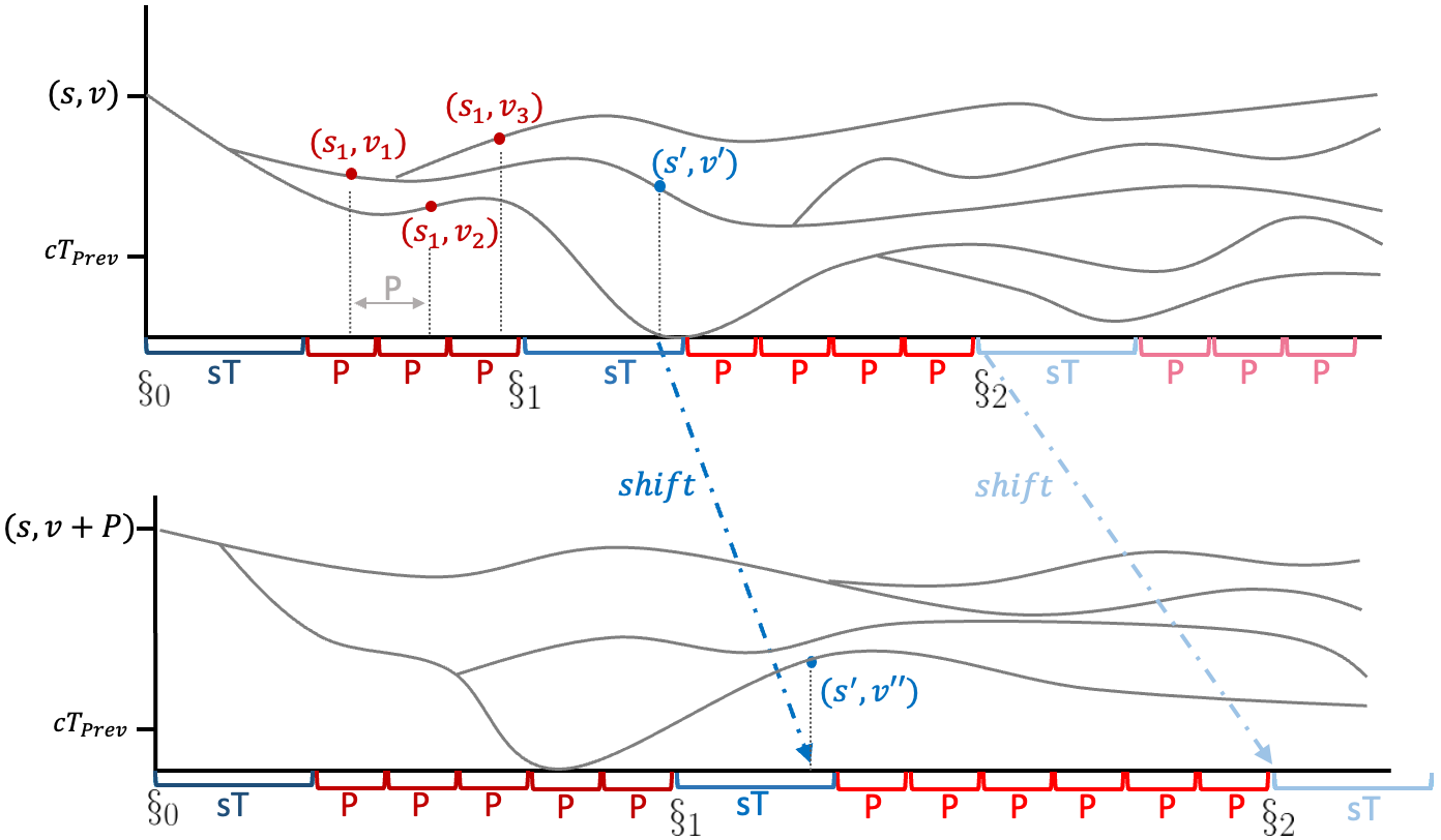
In order to prove Theorem 5.1, we show that every computation tree of ${\mathcal{A}}$ , starting from a big enough counter value $v>\texttt{cT}$ , has a ‘segmented periodic’ structure with respect to $\varphi$ . That is, we can divide its levels into $poly(n)$ many segments, such that only the first $\texttt{sT}\in Exp(n,|\varphi|$ ) levels in each segment are in the ‘core’, while every other level $\ell$ is a sort-of repetition of the level $\ell-\texttt{P}$ , for a period $\cP$ . We further show that there is a similarity between the cores of computation trees starting with counter values $v$ and $v+\texttt{P}$ . We depict the segmentation in Figure 2, and formalize it as follows.

Consider a formula $\varphi=\psi_{1}UA\psi_{2}$ , where $\psi_{1}$ and $\psi_{2}$ are $(\texttt{cT}(\psi_{1}),\texttt{P}(\psi_{1}))$ - and $(\texttt{cT}(\psi_{2}),\texttt{P}(\psi_{2}))$ -periodic, respectively. We define several constants to use throughout the proof.

Constants depending only on the number $n$ of states in the OCA
•

$b\in Poly(n)$ : the bound on the length of a linear path scheme on ${\mathcal{A}}$ .
•

$B=\mathrm{lcm}[1..2b^{3}]$ .
Constants depending on $n$ and the CTL+UA formula $\varphi$
•

${\texttt{P}_{prev}}(\varphi)=\mathrm{lcm}(\texttt{P}(\psi_{1}),\texttt{P}(\psi_{2}))$ – the unified period of the subformulas.
•

${\texttt{cT}_{prev}}(\varphi)=\max(\texttt{cT}(\psi_{1}),\texttt{cT}(\psi_{2}))$ – the unified counter threshold of the subformulas.
•

$\texttt{P}(\varphi)=B\cdot{\texttt{P}_{prev}}(\varphi)$ – the ‘period’ of $\varphi$ .
•

$\texttt{sT}(\varphi)=b^{9}\cdot\texttt{P}(\varphi)$ – the ‘segment threshold’ of $\varphi$ .
•

$\texttt{cT}(\varphi)=b^{11}\cdot\texttt{P}(\varphi)$ – the ‘counter threshold’ of $\varphi$ .

Eventually, these periodicity constants are plugged into the inductive cases of Theorem 3.3, as shown in the proof of Theorem 5.1. Then, all the constants are single-exponential in $n$ and the nesting depth of $\varphi$ . Notice that the following relationship holds between the constants.

Proposition 5.7.

$\texttt{P}(\varphi)>{\texttt{cT}_{prev}}(\varphi)$ for $b\geq 2$ .

When clear from the context, we omit the parameter $\varphi$ from $\texttt{P},\texttt{sT},\texttt{cT},{\texttt{P}_{prev}},{\texttt{cT}_{prev}}$ .

We provide below an intuitive explanation for the choice of constants above.

Intuition for the period P.

The period has two different roles: level-periodicity within each segment of a computation tree, and counter-value periodicity between two computation trees starting with different counter values.

Level periodicity within a segment: For lengthening or shortening a basic path by P, we add and/or remove some copies of its cycles. Adding or removing ${\texttt{P}_{prev}}$ copies of the same cycle guarantees that the end counter values of the original and new paths are equivalent modulo ${\texttt{P}_{prev}}$ . Since the cycles in a basic path are of length in $[0..b]$ , setting P to be divisible by ${\texttt{P}_{prev}}\cdot\mathrm{lcm}[1..b]$ , allows to add or remove $\frac{\texttt{P}}{|c|}$ copies of a cycle $c$ , where $\frac{\texttt{P}}{|c|}$ is divisible by ${\texttt{P}_{prev}}$ , as desired. Yet, we might need to add copies of one cycle and remove copies of another, thus, as per Proposition 5.6, we need P to be divisible by ${\texttt{P}_{prev}}\cdot lcm[1..2b^{2}]$ .

Counter periodicity between computation trees: We change a path $\tau$ that starts with a counter value $v$ to a path that starts with a counter value $v+\texttt{P}$ , or vice versa, by lengthening or shortening it by $\frac{\texttt{P}}{\texttt{s}}$ , respectively, where s is a positive basic slope. In some cases, we need to also make sure that the longer or shorter path has a drop bigger or smaller, respectively, than $\tau$ by exactly P.

As $\frac{\texttt{P}}{\texttt{s}}$ is bounded by $b\cdot\texttt{P}$ , if there are at least $b\cdot\texttt{P}$ repetitions of a cycle $c$ in $\tau$ whose slope is $-\texttt{s}$ , we can just add or remove $\frac{b\cdot\texttt{P}}{|c|}$ copies of $c$ , so we need P to be divisible by ${\texttt{P}_{prev}}\cdot\mathrm{lcm}[1..b]$ , for guaranteeing that the counter values at the end of the original and new paths are equivalent. Yet, in some cases we need to combine two cycles, as per Proposition 5.5. As the combination of the two cycles might be of length up to $2b^{3}$ , we need P to be divisible by ${\texttt{P}_{prev}}\cdot\mathrm{lcm}[1..2b^{3}]$ .

Intuition for the counter threshold cT and the segment threshold sT.

In order to apply Propositions 5.5 and 5.6, we need to have in the handled path many repetitions of two cycles of different slopes. We thus choose cT and sT to be large enough so that paths in which only one (negative) cycle slope is repeated many times must hit zero within a special region called the ‘core’ of the tree, as defined below.

The core of a computation tree.

For every counter value ${v}>\texttt{cT}$ , the ‘core’ with respect to a fixed formula $\varphi$ , denoted by $\texttt{core}({v})\subseteq\mathbb{N}$ , of a computation tree of ${\mathcal{A}}$ that starts with a counter value ${v}$ consists of $m+1<b^{2}$ segments, with each segment corresponding to a negative basic slope and having sT consequent numbers. For every $i\in[0..m]$ , the start of Segment $i$ depends on the initial counter value $v$ of the computation tree, it is denoted by $\mathsection_{i}(v)$ , and it is defined as follows:

•

$\mathsection_{0}(v)=0$ ,
•

For $i\in[1..m]$ , we set $\mathsection_{i}(v)=\frac{-1}{\texttt{s}_{i}}(v-{\texttt{cT}_{prev}})-b^{8}\cdot\texttt{P}$ .
•

For convenience, we also define $\mathsection_{m{+}1}(v)=\infty$ .

Then, we define $\texttt{core}(v)=\bigcup_{i=0}^{m}[\mathsection_{i}(v)..(\mathsection_{i}(v)+\texttt{sT}-1)]$ .

Observe that the core of every tree is an ordered list of $((m+1)\cdot\texttt{sT})$ numbers (levels), while just the starting level of every segment depends on the initial counter value $v$ . We can thus define a bijection $\textsf{shift}:\texttt{core}(v)\to\texttt{core}(v+\texttt{P})$ that maps the $i$ -th number in $\texttt{core}({v})$ to the $i$ -th number in $\texttt{core}({v+\texttt{P}})$ (see also Figure 2).

Recall that we define sT so that, intuitively, if a path is long enough to reach $\mathsection_{i}(v)+\texttt{sT}$ without reaching counter value ${\texttt{cT}_{prev}}$ , then the path must have many cycles with a slope larger than $\texttt{s}_{i}$ , and if the path manages to reach ${\texttt{cT}_{prev}}$ before $\mathsection_{i+1}(v)$ (namely the end of Segment $i$ ), then it must have many cycles with a slope at least as small as $\texttt{s}_{i}$ . This is formalized as follows.

Lemma 5.8.

Let $\tau$ be a basic path, or a prefix of it, of length $\ell$ starting from counter value $v>\texttt{cT}$ , and let $i\in[0..m]$ .

1.

If $\ell\geq\mathsection_{i}(v)+\frac{\texttt{sT}}{2}$ and the counter values of $\tau$ stay above ${cT_{prev}}$ , then $\tau$ has a cycle with slope $\texttt{s}_{j}$ for $j>i$ that repeats at least $b^{4}\cdot\texttt{P}$ times.
2.

If $\ell<\mathsection_{i+1}(v)$ and the counter values of $\tau$ reach ${cT_{prev}}$ , then $\tau$ has a cycle with slope $\texttt{s}_{j}$ for $j\leq i$ that repeats at least $b^{4}\cdot\texttt{P}$ times.

As a sanity check, the lemma states that if a path $\tau$ reaches ${\texttt{cT}_{prev}}$ for the first time at length $\ell\in[\mathsection_{1}(v){+}\frac{\texttt{sT}}{2}\leavevmode\nobreak\ ..\leavevmode\nobreak\ \mathsection_{2}(v))$ , then it has many cycles with slope $\texttt{s}_{1}=-1$ (enough to decrease down to ${\texttt{cT}_{prev}}$ before $\mathsection_{2}(v)$ ), as well as many cycle with slope at least $\texttt{s}_{2}=\frac{-(b-1)}{b}$ (enough to keep above ${\texttt{cT}_{prev}}$ through $\mathsection_{1}(v)+\frac{\texttt{sT}}{2}$ ). Observe also that a path cannot reach ${\texttt{cT}_{prev}}$ at Segment $0$ , namely before $\mathsection_{1}(v)$ .

The segment and shift periodicity.

Consider a threshold $T$ and period $P$ . We say that counter values $u,v$ are $(T,P)$ -equivalent, denoted by $u\equiv_{T,P}v$ if either $u,v\geq T$ and $P$ divides $|u-v|$ , or $u,v<T$ and $u=v$ . That is, either both $u,v$ are greater than $T$ , in which case they are equivalent modulo $P$ , or they are both smaller than $T$ and are equal.

The segment periodicity within a computation tree is then stated as Claim 1 in Lemma 5.9 below, while the similarity between computation trees starting from counters $v$ and $v+\texttt{P}$ as Claim 2. (By $(s,v)\stackrel{{\scriptstyle\ell}}{{\leadsto}}(s^{\prime},v^{\prime})$ we mean that the computation tree starting with state $s$ and counter value $v$ has a path of length $\ell$ ending in state $s^{\prime}$ and counter value $v^{\prime}$ .)

Lemma 5.9.

Consider states $s$ and $e$ , a counter value $v>\texttt{cT}$ , an arbitrary counter value $u$ , and an arbitrary path length $\ell$ .

1.
If $\ell\not\in\texttt{core}(v)$ then:
1. (a)
  
  $(s,v)\stackrel{{\scriptstyle\ell}}{{\leadsto}}(e,u)\implies(s,v)\stackrel{{\scriptstyle\ell-\texttt{P}}}{{\leadsto}}(e,u^{\prime})$ , and
2. (b)
  
  $(s,v)\stackrel{{\scriptstyle\ell-\texttt{P}}}{{\leadsto}}(e,u)\implies(s,v)\stackrel{{\scriptstyle\ell}}{{\leadsto}}(e,\tilde{u})$ ,
for some counter values $u^{\prime}$ and $\tilde{u}$ , such that $u\equiv_{{\texttt{cT}_{prev}},{\texttt{P}_{prev}}}u^{\prime}\equiv_{{\texttt{cT}_{prev}},{\texttt{P}_{prev}}}\tilde{u}$ .
2.
If $\ell\in\texttt{core}(v)$ then:
1. (a)
  
  $(s,v+\texttt{P})\stackrel{{\scriptstyle\textsf{shift}(\ell)}}{{\leadsto}}(e,u)\implies(s,v)\stackrel{{\scriptstyle\ell}}{{\leadsto}}(e,u^{\prime})$ , and
2. (b)
  
  $(s,v)\stackrel{{\scriptstyle\ell}}{{\leadsto}}(e,u)\implies(s,v+\texttt{P})\stackrel{{\scriptstyle\textsf{shift}(\ell)}}{{\leadsto}}(e,\tilde{u})$
for some counter values $u^{\prime}$ and $\tilde{u}$ , such that $u\equiv_{{\texttt{cT}_{prev}},{\texttt{P}_{prev}}}u^{\prime}\equiv_{{\texttt{cT}_{prev}},{\texttt{P}_{prev}}}\tilde{u}$ .

Throughout the proof, we will abbreviate $u\equiv_{{\texttt{cT}_{prev}},{\texttt{P}_{prev}}}u^{\prime}$ by $u\equiv u^{\prime}$ . We split the proof into four parts, each devoted to one of the four stated implications. In each of them, we assume the existence of a path $\tau$ that witnesses the left side of the implication, say $(s,v)\stackrel{{\scriptstyle\ell}}{{\leadsto}}(e,u)$ , and show that there exists a path $\tau^{\prime}$ that witnesses the right side of the implication, say $(s,v)\stackrel{{\scriptstyle\ell-\texttt{P}}}{{\leadsto}}(e,u^{\prime})$ , where $u\equiv u^{\prime}$ . By Lemma 3.4, we assume that $\tau$ is a basic path. We present some of the cases; the remaining parts are in the appendix.

Proof of Lemma 5.9.1a

Let $\tau$ be a basic path of length $\ell\notin\texttt{core}(v)$ such that $(s,v)\stackrel{{\scriptstyle\ell}}{{\leadsto}}(e,u)$ via $\tau$ . We construct from $\tau$ a path $\tau^{\prime}$ for $(s,v)\stackrel{{\scriptstyle\ell-\texttt{P}}}{{\leadsto}}(e,u^{\prime})$ , such that $u\equiv u^{\prime}$ . The proof is divided to two cases.

Case 1a.1: The counter values in $\tau$ stay above ${\texttt{cT}_{prev}}$

If there is no position in $\tau$ with counter value ${\texttt{cT}_{prev}}$ , then in particular $\tau$ has no zero-transitions. Since $\ell\notin\texttt{core}(v)$ , then in particular $\ell\geq\texttt{sT}>3b^{5}\texttt{P}$ . Thus, there are at least $3b^{4}\texttt{P}$ cycle repetitions in $\tau$ .

If there is a non-positive cycle $c$ that is repeated at least P times, we can obtain $\tau^{\prime}$ by removing $\frac{\texttt{P}}{|c|}$ copies of $c$ , as the counter values along $\tau^{\prime}$ are at least as high as the corresponding ones in $\tau$ . Observe that $\tau^{\prime}$ is of length $\ell-\texttt{P}$ from $(s,v)$ to $(e,u^{\prime})$ with $u^{\prime}=u-\emph{effect}(c)\frac{\texttt{P}}{|c|}$ . Since we have $u^{\prime}\geq u\geq{\texttt{cT}_{prev}}$ , then $u\equiv u^{\prime}$ .

Otherwise, each non-positive cycle in $\tau$ is taken at most P times. Thus, the positive cycles are repeated at least $3b^{4}\texttt{P}-b\texttt{P}\geq 3b^{3}\texttt{P}$ times. In particular, there exists a positive cycle $c$ that repeats at least $3b^{2}\texttt{P}$ times. By removing $\frac{\texttt{P}}{|c|}$ occurrences of it, we obtain a path $\tau^{\prime}$ of length $\ell-\texttt{P}$ . Notice first that this path is valid. Indeed, up until the cycle $c$ is taken, the path $\tau^{\prime}$ coincides with $\tau$ , so the counter remains above ${\texttt{cT}_{prev}}$ . Since $c$ is a positive cycle, after completing its iterations, the counter value becomes at least $3b^{2}\texttt{P}-\texttt{P}+{\texttt{cT}_{prev}}$ . Then, even if all remaining transitions in the negative cycles have effect $-1$ , the counter value is reduced by at most $b^{2}\texttt{P}$ (as there are at most $(b-1)\texttt{P}$ remaining cycles, each of effect at least $-b$ , and the simple paths in $\tau$ can reduce by another $b$ at most). Thus, the value of the counter remains at least $3b^{2}\texttt{P}-\texttt{P}+{\texttt{cT}_{prev}}-b^{2}\texttt{P}>{\texttt{cT}_{prev}}$ . Finally, let $(e,u^{\prime})$ be the configuration reached at the end of $\tau^{\prime}$ , then $u-u^{\prime}=\emph{effect}(c)\frac{\texttt{P}}{|c|}$ , so $u\equiv u^{\prime}$ .

Case 1a.2: $\tau$ reaches counter value ${\texttt{cT}_{prev}}$ .

Let $0\leq z_{f}\leq z_{u}\leq\ell$ be the first and ultimate positions in $\tau$ where the counter value is exactly ${\texttt{cT}_{prev}}$ . We split $\tau$ into three parts: $\tau_{1}=\tau[0\leavevmode\nobreak\ ..\leavevmode\nobreak\ z_{f}),\tau_{2}=\tau[z_{f}\leavevmode\nobreak\ ..\leavevmode\nobreak\ z_{u}),\tau_{3}=\tau[z_{u}\leavevmode\nobreak\ ..\leavevmode\nobreak\ \ell]$ (it could be that $z_{f}=z_{u}$ , in which case the middle part is empty). Since $\tau$ is of length $\ell\geq\texttt{sT}\geq b^{9}\cdot\texttt{P}$ , then at least one of the parts above is of length at least $b^{8}\cdot\texttt{P}$ (recall $b\geq 3$ ). We split according to which part that is. For simplicity, we start with the cases that $\tau_{2}$ or $\tau_{3}$ are long, and only then handle the case of a long $\tau_{1}$ .

1.

The middle part $\tau_{2}=\tau[z_{f}\leavevmode\nobreak\ ..\leavevmode\nobreak\ z_{u}]$ is of length at least $b^{8}\cP$ .

As $\tau_{2}$ is of length at least $b^{8}\cdot\texttt{P}$ , some cycle $c$ in it must repeat at least $b^{6}\cdot\texttt{P}$ times.

If $c$ is balanced, we can obtain $\tau^{\prime}$ by removing $\frac{\texttt{P}}{|c|}$ of its repetitions.

If $c$ is positive, starting at position $x$ with counter value $v_{x}$ , then the counter value at position $y$ where $c$ ’s repetitions end is at least $v_{x}+b^{6}\cdot\texttt{P}$ . As $\tau_{2}$ eventually gets down to ${\texttt{cT}_{prev}}<\texttt{P}$ , there must be a negative cycle $c_{-}$ that repeats at least $b\cdot\texttt{P}$ times between position $y$ and the first position after $y$ that has the counter value $v_{x}+\frac{b^{6}\cdot\texttt{P}}{2}$ . Hence, we can obtain $\tau^{\prime}$ by removing repetitions of $c$ and $c_{-}$ , as per Proposition 5.6, ensuring that the only affected values are above $v_{x}$ .

If $c$ is negative, starting at position $x$ with counter value $v_{x}$ , then $v_{x}\geq b^{6}\cdot\texttt{P}$ . As $\tau_{2}$ starts with counter value ${\texttt{cT}_{prev}}$ , and ${\texttt{cT}_{prev}}<P$ (Proposition 5.7), there must be a positive cycle $c_{+}$ that repeats at least $b\cdot\texttt{P}$ times between the last position with counter value $\frac{b^{6}\cdot\texttt{P}}{2}$ and $x$ . Hence, we can obtain $\tau^{\prime}$ by removing repetitions of $c$ and $c_{+}$ , as per Proposition 5.6, ensuring that the only affected values are above $b^{5}\cdot\texttt{P}$ .
2.

The last part $\tau_{3}=\tau[z_{u}\leavevmode\nobreak\ ..\leavevmode\nobreak\ \ell]$ is of length at least $b^{8}\cP$ .

As in the previous case, a cycle $c$ must repeat in $\tau_{3}$ at least $b^{6}\cdot\texttt{P}$ times. If $c$ is balanced, we can remove $\frac{\texttt{P}}{|c|}$ of its repetitions, getting the desired path $\tau^{\prime}$ .

Otherwise, it must be that $\tau_{3}$ stays above ${\texttt{cT}_{prev}}$ , and reaches a value at least $b^{6}\cdot\texttt{P}$ . Indeed, if $c$ is positive then its repetitions end at some position $x$ with a counter value at least that high, and if it is negative it starts at some position $x$ with a counter value at least that high.

If the counter value also drops to $\frac{b^{6}\cdot\texttt{P}}{2}$ after position $x$ , then we can remove positive and negative cycles exactly as in the previous case. Otherwise, we can just remove $\frac{\texttt{P}}{|c|}$ repetitions of $c$ , guaranteed that the counter value at the end of $\tau_{3}$ is above ${\texttt{cT}_{prev}}$ .
3.

Only the first part $\tau_{1}=\tau[0\leavevmode\nobreak\ ..\leavevmode\nobreak\ z_{f})$ is of length at least $b^{8}\cP$ .

If any of the other parts is long, we shorten them. Otherwise, their combined length is less than $2b^{8}\cdot\texttt{P}<\frac{\texttt{sT}}{2}$ , implying that the first part $\tau_{1}$ is longer than $\mathsection_{i}(v)+\frac{\texttt{sT}}{2}$ .

Hence, by Lemma 5.8, there are ‘fast’ and ‘slow’ cycles $c_{f}$ and $c_{s}$ , respectively, of slopes $\texttt{s}_{f}<\texttt{s}_{s}$ , such that each of them repeats at least $b^{4}\cdot\texttt{P}$ times in $\tau_{1}$ .
Thus, by Proposition 5.6, we can add and/or remove some repetitions of $c_{f}$ and $c_{s}$ , such that $\tau_{1}$ is shorten by exactly P. Yet, we should ensure that the resulting path $\tau^{\prime}$ is valid, in the sense that its corresponding first part $\tau^{\prime}_{1}$ cannot get the counter value to $0$ . We show it by cases:
- •
  
  If $c_{f}$ or $c_{s}$ are balanced cycles, then we can remove the balanced cycle only, without changing the remaining counter values.
- •
  
  If there is a positive cycle $c_{+}$ that repeats at least $2b^{2}\cdot\texttt{P}$ times, then the counter value climbs by at least $2b^{2}\cdot\texttt{P}$ from its value $v_{x}$ at position $x$ where $c_{+}$ starts and the position $y$ where its repetitions end. As the counter gets down to ${\texttt{cT}_{prev}}$ at the end of $\tau_{1}$ , and ${\texttt{cT}_{prev}}<P$ (Proposition 5.7), there must be a negative cycle $c_{-}$ that repeats at least $b\cdot\texttt{P}$ times between position $y$ and the first position after $y$ that has the counter value $v_{x}+b^{2}\cdot\texttt{P}$ . Hence, we can remove repetitions of $c_{+}$ and $c_{-}$ , as per Proposition 5.6, ensuring that the only affected values are above $v_{x}$ .
- •
  Otherwise, both $c_{f}$ and $c_{s}$ are negative, implying that we add some repetitions of $c_{f}$ and remove some repetitions of $c_{s}$ . We further split into two subcases:
  - –
    
    If $c_{s}$ appears before $c_{f}$ then there is no problem, as the only change of values will be their increase, and all the values were nonzero to begin with (as we are before $z_{f}$ ).
  - –
    
    If $c_{f}$ appears first, ending at some position $x$ , while $c_{s}$ starts at some later position $y$ , then a-priori it might be that repeating $c_{f}$ up to $b\cdot\texttt{P}$ more times, as per Proposition 5.6, will take the counter value to $0$ .
    
    However, observe that since there are at most $b-2$ positive cycles, and each of them can repeat at most $2b^{2}\cdot\texttt{P}-1$ times, the counter value $v_{x}$ at position $x$ , and along the way until position $y$ , is at least $v_{y}-(b-2)2b^{2}\cdot\texttt{P}$ , where $v_{y}$ is the counter value at position $y$ . As $c_{s}$ repeats at least $b^{4}\cdot\texttt{P}$ times, we have $v_{y}\geq b^{4}\cdot\texttt{P}$ . Thus $v_{x}\geq b^{4}\cdot\texttt{P}-2(b-2)b^{2}\cdot\texttt{P}>b^{2}\texttt{P}$ . Hence, repeating $c_{f}$ up to $b\cdot\texttt{P}$ more times at position $x$ cannot take the counter value to $0$ , until position $y$ , as required.

Proof of Lemma 5.9.2a

The case of Segment $\mathsection_{0}$ .

For a path of length $\ell$ , we have in Segment $0$ that $\textsf{shift}(\ell)=\ell$ , and indeed a path from $v$ is valid from $v+\texttt{P}$ and vise versa, as they do not hit ${\texttt{cT}_{prev}}$ : Their maximal drop is sT, while $v\geq\texttt{cT}>\texttt{P}+\texttt{sT}>{\texttt{cT}_{prev}}+\texttt{sT}$ .

We turn to the $i$ th segment, for $i\geq 1$ . Consider a basic path $\tau$ for $(s,v+\texttt{P})\stackrel{{\scriptstyle\textsf{shift}(\ell)}}{{\leadsto}}(e,u)$ . Recall that $\textsf{shift}(\ell)=\ell+\frac{\texttt{P}}{-\texttt{s}_{i}}\in[\mathsection_{i}(v+\texttt{P})\leavevmode\nobreak\ ..\leavevmode\nobreak\ \mathsection_{i}(v+\texttt{P})+\texttt{sT})]$ . We construct from $\tau$ a path $\tau^{\prime}$ for $(s,v)\stackrel{{\scriptstyle\ell}}{{\leadsto}}(e,u^{\prime})$ , such that $u\equiv u^{\prime}$ , along the following cases.

Case 2a.1: The counter values in $\tau$ stay above ${\texttt{cT}_{prev}}$

As there is no position in $\tau$ with counter value ${\texttt{cT}_{prev}}$ , then in particular $\tau$ has no zero-transitions. We further split into two subcases:

1.

If $\tau$ does not have $b\cdot\texttt{P}$ repetitions of a ‘relatively fast’ cycle with slope $\texttt{s}_{j}$ for $j\leq i$ , then the drop of $\tau$ , and of every prefix of it, is at most $X+Y$ , where $X$ stands for the drop outside ‘slow’ cycles of slope $\texttt{s}_{h}$ for $h>i$ , and $Y$ for the rest of the drop. We have $X<b^{3}\cdot\texttt{P}$ and $Y<(\ell+\frac{\texttt{P}}{\texttt{s}_{i}})(-\texttt{s}_{i+1})$ .

We claim that we can obtain $\tau^{\prime}$ by removing $\frac{\texttt{P}}{-\texttt{s}_{i}\cdot|c|}$ repetitions of any cycle $c$ , which repeats enough in $\tau$ , having that the drop $D$ of $\tau^{\prime}$ is less than $v-{\texttt{cT}_{prev}}$ .

Indeed, the maximal such drop $D$ might be the result of removing only cycles of slope $(+1)$ , whose total effect is $\frac{\texttt{P}}{-\texttt{s}_{i}}$ , having $D\leq\frac{\texttt{P}}{-\texttt{s}_{i}}+X+Y=\frac{\texttt{P}}{-\texttt{s}_{i}}+b^{3}\cdot\texttt{P}+(\ell+\frac{\texttt{P}}{-\texttt{s}_{i}})(-\texttt{s}_{i+1})\leq b\cdot\texttt{P}+b^{3}\cdot\texttt{P}+(\ell+\frac{\texttt{P}}{-\texttt{s}_{i}})(-\texttt{s}_{i+1}).$ Since $\ell<\mathsection_{i+1}(v+\texttt{P})=\frac{1}{-\texttt{s}_{i+1}}(v+\texttt{P}-{\texttt{cT}_{prev}})-b^{8}\cdot\texttt{P}$ , we have $D\leq(b^{3}+b)\cdot\texttt{P}+(\frac{1}{-\texttt{s}_{i+1}}(v+\texttt{P}-{\texttt{cT}_{prev}})-b^{8}\cdot\texttt{P})+\frac{\texttt{P}}{-\texttt{s}_{i}})(-\texttt{s}_{i+1})=$
$(b^{3}+b)\cdot\texttt{P}+v+\texttt{P}-{\texttt{cT}_{prev}}-(-\texttt{s}_{i+1})\cdot b^{8}\cdot\texttt{P}+\frac{(-\texttt{s}_{i+1})}{-\texttt{s}_{i}}\cdot\texttt{P})=(b^{3}+b+1+\frac{(-\texttt{s}_{i+1})}{-\texttt{s}_{i}})\cdot\texttt{P}+v-{\texttt{cT}_{prev}}-(-\texttt{s}_{i+1})\cdot b^{8}\cdot\texttt{P})<b^{4}\cdot\texttt{P}-b^{7}\cdot\texttt{P}+v-{\texttt{cT}_{prev}}.$ It is thus left to show that $b^{4}\cdot\texttt{P}<b^{7}\cdot\texttt{P}$ , which obviously holds.
2.

Otherwise, namely when $\tau$ does have $b\cdot\texttt{P}$ repetitions of a ‘relatively fast’ cycle with slope $\texttt{s}_{j}$ for $j\leq i$ , let $c$ be the first such cycle in $\tau$ . We can obtain $\tau^{\prime}$ by removing $\frac{\texttt{P}}{-\texttt{s}_{i}\cdot|c|}$ repetitions of $c$ : The counter value in $\tau^{\prime}$ , which starts with counter value $v$ , at the position after the repetitions of $c$ will be at least as high as the counter value in $\tau$ , which starts with counter value $v+\texttt{P}$ , after the repetitions of $c$ . Notice that the counter value cannot hit ${\texttt{cT}_{prev}}$ before arriving to the repetitions of $c$ by the argument of the previous subcase.

Case 2a.2: $\tau$ reaches counter value ${\texttt{cT}_{prev}}$

Again let $\tau_{1}=\tau[0\leavevmode\nobreak\ ..\leavevmode\nobreak\ z_{f}),\tau_{2}=\tau[z_{f}\leavevmode\nobreak\ ..\leavevmode\nobreak\ z_{u}),\tau_{3}=\tau[z_{u}\leavevmode\nobreak\ ..\leavevmode\nobreak\ \textsf{shift}(\ell)]$ as in 1a.

In order to handle possible zero transitions, we shorten $\tau_{1}$ , such that the resulting first part $\tau^{\prime}_{1}$ of $\tau^{\prime}$ , which starts with counter value $v$ , also ends with counter value exactly ${\texttt{cT}_{prev}}$ . Since $\tau_{1}$ reaches ${\texttt{cT}_{prev}}$ and is shorter than $\mathsection_{i+1}(v+\texttt{P})$ , it has by Lemma 5.8.2 at least $b^{4}\cdot\texttt{P}$ repetitions of a ‘fast’ cycle of slope $\texttt{s}_{f}\leq\texttt{s}_{i}$ . Let $c_{f}$ be the first such cycle. We split to cases.

1.

If $\texttt{s}_{f}=\texttt{s}_{i}$ or $\tau_{2}$ or $\tau_{3}$ are of length at least $b^{5}\cdot\texttt{P}$ , we can remove $\frac{\texttt{P}}{-\texttt{s}_{f}\cdot|c_{f}|}$ repetitions of $c_{f}$ in $\tau_{1}$ . Note that the resulting first part $\tau^{\prime}_{1}$ of $\tau^{\prime}$ indeed ends with counter value ${\texttt{cT}_{prev}}$ . However, while when $\texttt{s}_{f}=\texttt{s}_{i}$ the resulting length of $\tau^{\prime}$ will be $\ell$ , as required, in the case that $\texttt{s}_{f}<\texttt{s}_{i}$ , we have that $\tau^{\prime}$ will be longer than $\ell$ . Nevertheless, in this case, as $\tau_{2}$ or $\tau_{3}$ are of length at least $b^{5}\cdot\texttt{P}$ , we can further shorten $\tau_{2}$ or $\tau_{3}$ without changing their effect, as per Proposition 5.6, analogously to 1 or 2, respectively, in the proof of Lemma 5.9.1a.2.
2.

Otherwise, we are in the case that $\tau_{1}$ has a ‘really fast’ cycle of slope $\texttt{s}_{f}<\texttt{s}_{i}$ that repeats at least $b^{4}\cdot\texttt{P}$ times, and both $\tau_{2}$ or $\tau_{3}$ are of length less than $b^{5}\cdot\texttt{P}$ . We claim that in this case $\tau_{1}$ must also have $b^{4}\cdot\texttt{P}$ repetitions of a ‘relatively slow’ cycle $c_{s}$ of slope $\texttt{s}_{s}\geq\texttt{s}_{i}$ .

Indeed, assume toward contradiction that $\tau_{1}$ has less than $b^{4}\cdot\texttt{P}$ repetitions of a cycle with slope $\texttt{s}_{s}$ for $s\geq i$ . Then the longest such path has less than $b$ transitions of $(+1)$ out of cycles, $b^{6}\cdot\texttt{P}$ such transitions in cycles, and the rest of it consists of ‘fast’ cycles with slope indexed lower than $i$ .

Thus its length is at most $X+L$ , where $X=b^{6}\cdot\texttt{P}$ is the $(+1)$ transitions, and $L$ is the longest length to drop from counter value $v+\texttt{P}+X$ to ${\texttt{cT}_{prev}}$ with ‘fast’ cycles. Thus, $L\leq\frac{1}{-\texttt{s}_{i-1}}(v+\texttt{P}+X-{\texttt{cT}_{prev}})$ .

Now, we have that the length of $\tau$ is at least $\mathsection_{i}(v+\texttt{P})=\frac{1}{-\texttt{s}_{i}}(v-{\texttt{cT}_{prev}})-b^{8}\cdot\texttt{P}$ . Thus, parts $\tau_{2}$ and $\tau_{3}$ of $\tau$ are of length at least $Z=\frac{1}{-\texttt{s}_{i}}(v-{\texttt{cT}_{prev}})-b^{8}\cdot\texttt{P}-\frac{1}{-\texttt{s}_{i-1}}(v+\texttt{P}+X-{\texttt{cT}_{prev}})-X=(\frac{1}{-\texttt{s}_{i}}-\frac{1}{-\texttt{s}_{i+1}})(v-{\texttt{cT}_{prev}})-b^{8}\cdot\texttt{P}-(1+\frac{1}{-\texttt{s}_{i+1}})b^{6}\cdot\texttt{P}$ .

Since $(\frac{1}{-\texttt{s}_{i}}-\frac{1}{-\texttt{s}_{i+1}})\geq\frac{1}{b^{2}}$ , $(1+\frac{1}{-\texttt{s}_{i+1}}\leq b+1)$ , and $v-{\texttt{cT}_{prev}}\geq\texttt{cT}-{\texttt{cT}_{prev}}>\texttt{cT}-\texttt{P}>3b^{10}\texttt{P}$ , we have $Z\geq\frac{1}{b^{2}}(3b^{10}\cdot\texttt{P})-b^{8}\cdot\texttt{P}-(b+1)b^{6}\cdot\texttt{P}=2b^{8}\cdot\texttt{P}-(b+1)b^{6}\cdot\texttt{P}$ . Therefore, at least one of $\tau_{2}$ and $\tau_{3}$ is of length at least $b^{7}\cdot\texttt{P}$ , leading to a contradiction.

So, we are in the case that $\tau_{1}$ has at least $b^{4}\cdot\texttt{P}$ repetitions of a ‘really fast’ cycle $c_{f}$ of slope $\texttt{s}_{f}<\texttt{s}_{i}$ as well as $b^{4}\cdot\texttt{P}$ repetitions of a ‘relatively slow’ cycle $c_{s}$ of slope $\texttt{s}_{s}\geq\texttt{s}_{i}$ .

By analyzing the different possible orders of $c_{s}$ and $c_{f}$ , we can cut and repeat the cycles far enough from 0 so as to construct valid paths. See the Appendix for details.∎

5.1 Proof of Theorem 5.1

The proof is by induction over the structure of $\varphi$ , where Theorem 3.3 already provides the periodicity for all CTL operators.

It remains to plug $UA$ into the induction by showing (1) the $(\texttt{cT},\texttt{P})$ -periodicity of a formula $\varphi=\psi_{1}UA\psi_{2}$ with respect to an OCA ${\mathcal{A}}$ , provided that its subformulas are $({\texttt{cT}_{prev}},{\texttt{P}_{prev}})$ -periodic; and (2) by showing that the period P and threshold cT are single-exponential in $n=|{\mathcal{A}}|$ and in the nesting depth of $\varphi$ .

1.

We show that for every state $s\in S$ and counters $v,v^{\prime}>\texttt{cT}$ , if $v\equiv v^{\prime}\mod\texttt{P}$ then $(s,v)\models\varphi\iff(s,v^{\prime})\models\varphi$ . Withot loss of generality, write $v^{\prime}=v+z\cdot\texttt{P}$ , for some $z\in\mathbb{N}$ .

• If $(s,v)\models\varphi$ then by the definition of the $AU$ operator and the completeness of ${\mathcal{A}}$ we have i) there is a level $\ell$ , such that for every state $e$ and counter value $u$ , if $(s,v)\stackrel{{\scriptstyle\ell}}{{\leadsto}}(e,u)$ then $(e,u)\models\psi_{2}$ , and ii) for every level $m<\ell$ , state $h$ and counter value $x$ , if $(s,v)\stackrel{{\scriptstyle m}}{{\leadsto}}(h,x)$ then $(h,x)\models\psi_{1}$ .

Observe first that if $\ell\not\in\texttt{core}(v)$ , then there also exists a level $\hat{\ell}<\ell$ witnessing $(s,v)\models\varphi$ , such that $\hat{\ell}\in\texttt{core}(v)$ . Indeed, we obtain $\hat{\ell}$ , by choosing the largest level $\hat{\ell}$ in the core of $\ell$ ’s segment, such that $\ell\equiv\hat{\ell}\mod\texttt{P}$ . As $\hat{\ell}<\ell$ , it directly follows that for every level $\hat{m}<\hat{\ell}$ , state $\hat{h}$ and counter value $\hat{x}$ , if $(s,v)\stackrel{{\scriptstyle\hat{m}}}{{\leadsto}}(\hat{h},\hat{x})$ then $(\hat{h},\hat{x})\models\psi_{1}$ . Now, assume toward contradiction that there is a state $\hat{e}$ and a counter value $\hat{u}$ , such that $(s,v)\stackrel{{\scriptstyle\hat{\ell}}}{{\leadsto}}(\hat{e},\hat{u})$ and $(\hat{e},\hat{u})\not\models\psi_{2}$ . Then by (possibly several applications of) Lemma 5.9.1b, there is also a counter value $\hat{\hat{u}}\equiv_{{\texttt{cT}_{prev}},{\texttt{P}_{prev}}}\hat{u}$ , such that $(s,v)\stackrel{{\scriptstyle\ell}}{{\leadsto}}(\hat{e},\hat{\hat{u}})$ . As $\psi_{2}$ is $({\texttt{cT}_{prev}},{\texttt{P}_{prev}})$ -periodic, we have $(\hat{e},\hat{\hat{u}})\not\models\psi_{2}$ , leading to a contradiction.

Next, we claim that the level ${\ell^{\prime}}=\textsf{shift}^{z}(\hat{\ell})$ , obtained by $z$ (recall that $z=\frac{v^{\prime}-v}{\texttt{P}}$ ) applications of the shift function on $\hat{\ell}$ , witnesses $(s,v^{\prime})\models\varphi$ , namely that i) for every state $e^{\prime}$ and counter value $u^{\prime}$ , if $(s,v^{\prime})\stackrel{{\scriptstyle\ell^{\prime}}}{{\leadsto}}(e^{\prime},u^{\prime})$ then $(e^{\prime},u^{\prime})\models\psi_{2}$ , and ii) for every level $m^{\prime}<\ell^{\prime}$ , state $h^{\prime}$ and counter value $x^{\prime}$ , if $(s,v^{\prime})\stackrel{{\scriptstyle m^{\prime}}}{{\leadsto}}(h^{\prime},x^{\prime})$ then $(h^{\prime},x^{\prime})\models\psi_{1}$ .

Indeed, i) were it the case that $(e^{\prime},u^{\prime})\not\models\psi_{2}$ then by ( $z$ applications of) Lemma 5.9.2a, there was also a counter value $u^{\prime\prime}\equiv_{{\texttt{cT}_{prev}},{\texttt{P}_{prev}}}u^{\prime}$ , such that $(s,v)\stackrel{{\scriptstyle\hat{\ell}}}{{\leadsto}}(e^{\prime},u^{\prime\prime})$ and therefore $(e^{\prime},u^{\prime\prime})\not\models\psi_{2}$ , leading to a contradiction; and ii) were it the case that $(s,v^{\prime})\stackrel{{\scriptstyle m^{\prime}}}{{\leadsto}}(h^{\prime},x^{\prime})$ and $(h^{\prime},x^{\prime})\not\models\psi_{1}$ then a) by Lemma 5.9.1a, as in the argument above, there is also a level $\tilde{m}\leq m^{\prime}$ , such that $\tilde{m}$ is in the core of $m^{\prime}$ ’s segment and $(s,v^{\prime})\stackrel{{\scriptstyle\tilde{m}}}{{\leadsto}}(h^{\prime},\tilde{x})$ where $\tilde{x}\equiv_{{\texttt{cT}_{prev}},{\texttt{P}_{prev}}}x$ , and b) by Lemma 5.9.2a there is a level $\hat{m}<\hat{\ell}$ , such that $(s,v)\stackrel{{\scriptstyle\hat{m}}}{{\leadsto}}(h^{\prime},\hat{x})$ where $\hat{x}\equiv_{{\texttt{cT}_{prev}},{\texttt{P}_{prev}}}x$ and therefore $(h^{\prime},\hat{x})\not\models\psi_{1}$ , leading to a contradiction.

• If $(s,v^{\prime})\models\varphi$ then we have $(s,v)\models\varphi$ by an argument analogous to the above, while using Lemma 5.9.2b instead of Lemma 5.9.2a.
2.

The threshold cT and period P are calculated along the induction on the structure of the formula $\varphi$ . They start with threshold $0$ and period $1$ , and their increase in each step of the induction depends on the outermost operator.

Observe first that we can take as the worst case the same increase in every step, that of the UA case, since it guarantees the others. Namely, its required threshold, based on the threshold and period of the subformulas, is bigger than the threshold required in the other cases, and its required period is divisible by the periods required for the other cases.

Next, notice that both the threshold and period in the UA case only depend on the periods of the subformulas (i.e., not on their thresholds), so it is enough to show that the period is singly exponential in $n$ and the nesting depth of $\varphi$ .

The period in the UA case is defined to be $\texttt{P}(\varphi)=B\cdot\mathrm{lcm}(\texttt{P}(\psi_{1}),\texttt{P}(\psi_{2}))$ , where $B=\mathrm{lcm}[1..2b^{3}]$ , and $b$ is the bound on the length of a linear path scheme for ${\mathcal{A}}$ . By [17], $b$ is polynomial in $n$ , and as $\mathrm{lcm}[1..2b^{3}]<4^{2b^{3}}$ , we get that $B$ is singly exponential in $n$ .

Considering $\mathrm{lcm}(\texttt{P}(\psi_{1}),\texttt{P}(\psi_{2})$ , while in general $\mathrm{lcm}(x,y)$ of two numbers $x$ and $y$ might be equal to their multiplication, in our case, as both $\psi_{1}$ and $\psi_{2}$ are calculated along the induction via the same scheme above, they are both an exponent of $B$ . Hence, $\mathrm{lcm}(\texttt{P}(\psi_{1}),\texttt{P}(\psi_{2})=\max(\texttt{P}(\psi_{1}),\texttt{P}(\psi_{2})$ . Thus, we get that $\texttt{P}(\varphi)\leq B^{x}$ , where $x$ is bounded by the nesting depth of $\varphi$ . ∎

References

[1] Shaull Almagor, Udi Boker, and Orna Kupferman. Formalizing and reasoning about quality. Journal of the ACM, 63(3):24:1–24:56, 2016.
[2] Roland Axelsson, Matthew Hague, Stephan Kreutzer, Martin Lange, and Markus Latte. Extended computation tree logic. In Logic for Programming, Artificial Intelligence, and Reasoning: 17th International Conference, LPAR-17, Yogyakarta, Indonesia, October 10-15, 2010. Proceedings 17, pages 67–81. Springer, 2010.
[3] Udi Boker, Krishnendu Chatterjee, Thomas A. Henzinger, and Orana Kupferman. Temporal specifications with accumulative values. ACM Trans. Comput. Log., 15(4):27:1–27:25, 2014.
[4] Krishnendu Chatterjee and Laurent Doyen. Computation tree logic for synchronization properties. In Ioannis Chatzigiannakis, Michael Mitzenmacher, Yuval Rabani, and Davide Sangiorgi, editors, 43rd International Colloquium on Automata, Languages, and Programming, ICALP 2016, July 11-15, 2016, Rome, Italy, volume 55 of LIPIcs, pages 98:1–98:14. Schloss Dagstuhl - Leibniz-Zentrum für Informatik, 2016.
[5] Michael R Clarkson, Bernd Finkbeiner, Masoud Koleini, Kristopher K Micinski, Markus N Rabe, and César Sánchez. Temporal logics for hyperproperties. In Principles of Security and Trust: Third International Conference, POST 2014, Held as Part of the European Joint Conferences on Theory and Practice of Software, ETAPS 2014, Grenoble, France, April 5-13, 2014, Proceedings 3, pages 265–284. Springer, 2014.
[6] Michael R Clarkson and Fred B Schneider. Hyperproperties. Journal of Computer Security, 18(6):1157–1210, 2010.
[7] Byron Cook, Heidy Khlaaf, and Nir Piterman. Verifying increasingly expressive temporal logics for infinite-state systems. Journal of the ACM (JACM), 64(2):1–39, 2017.
[8] David C Cooper. Theorem proving in arithmetic without multiplication. Machine intelligence, 7(91-99):300, 1972.
[9] Stéphane Demri, Alain Finkel, Valentin Goranko, and Govert van Drimmelen. Model-checking CTL* over flat Presburger counter systems. Journal of Applied Non-Classical Logics, 20(4):313–344, 2010.
[10] Alain Finkel, Jérôme Leroux, and Grégoire Sutre. Reachability for two-counter machines with one test and one reset. In FSTTCS 2018-38th IARCS Annual Conference on Foundations of Software Technology and Theoretical Computer Science, volume 122, pages 31–1. Schloss Dagstuhl-Leibniz-Zentrum fuer Informatik, 2018.
[11] Michael J Fischer and Michael O Rabin. Super-exponential complexity of Presburger arithmetic. In Quantifier Elimination and Cylindrical Algebraic Decomposition, pages 122–135. Springer, 1998.
[12] Seymour Ginsburg and Edwin H Spanier. Bounded ALGOL-like languages. Transactions of the American Mathematical Society, 113(2):333–368, 1964.
[13] Stefan Göller and Markus Lohrey. Branching-time model checking of one-counter processes and timed automata. SIAM J. Comput., 42(3):884–923, 2013.
[14] Christoph Haase. A survival guide to Presburger arithmetic. ACM SIGLOG News, 5(3):67–82, 2018.
[15] Christoph Haase, Stephan Kreutzer, Joël Ouaknine, and James Worrell. Reachability in succinct and parametric one-counter automata. In CONCUR 2009-Concurrency Theory: 20th International Conference, CONCUR 2009, Bologna, Italy, September 1-4, 2009. Proceedings 20, pages 369–383. Springer, 2009.
[16] Jérôme Leroux and Grégoire Sutre. Flat counter automata almost everywhere! In International Symposium on Automated Technology for Verification and Analysis, pages 489–503. Springer, 2005.
[17] Jérôme Leroux and Grégoire Sutre. Reachability in two-dimensional vector addition systems with states: One test is for free. In 31st International Conference on Concurrency Theory (CONCUR 2020). Schloss Dagstuhl-Leibniz-Zentrum für Informatik, 2020.
[18] Marvin L. Minsky. Computation: Finite and Infinite Machines. Prentice-Hall, Englewood Cliffs, N.J., 1967.
[19] Mohan Nair. On chebyshev-type inequalities for primes. The American Mathematical Monthly, 89(2):126–129, 1982.
[20] Mojzesz Presburger. Über die Vollständigkeit eines gewissen Systems der Arithmetik ganzer Zahlen, in welchem die Addition als einzige Operation hervortritt. Comptes Rendus du I Congrès de Mathématiciens des Pays Slaves, pages 92–101, 1929.
[21] Leslie G Valiant and Michael S Paterson. Deterministic one-counter automata. Journal of Computer and System Sciences, 10(3):340–350, 1975.
[22] Igor Walukiewicz. Model checking CTL properties of pushdown systems. In International Conference on Foundations of Software Technology and Theoretical Computer Science, pages 127–138. Springer, 2000.

Appendix A Appendix – Omitted Proofs

A.1 Proofs for Sections 3 and 4

Proof A.1 (Proof of Proposition 3.1).

By definition, if $\varphi$ is totally $(\mathtt{t}(\varphi),\mathtt{p}(\varphi))$ -periodic then so is every subformula. We show the converse.

Denote by $\mathsf{subs}$ the set of subformulas of $\varphi$ . Assume that every $\psi\in\mathsf{subs}$ is $(\mathtt{t}(\psi),\mathtt{p}(\psi))$ -periodic for some constants $\mathtt{t}^{\prime}(\psi),\mathtt{p}^{\prime}(\psi)$ . Let $\mathtt{t}(\varphi)=\max\{\mathtt{t}^{\prime}(\psi)\mid\psi\in\mathsf{subs}\}$ and $\mathtt{p}(\varphi^{\prime})=\mathrm{lcm}(\{\mathtt{p}(\psi)\mid\psi\in\mathsf{subs}\})$ . We claim that $\varphi$ is totally $(\mathtt{t}(\varphi),\mathtt{p}(\varphi))$ -periodic. Indeed, this follows from the simple observation that if $\psi$ is $(\mathtt{t}^{\prime}(\psi),\mathtt{p}^{\prime}(\psi))$ -periodic, then it is also $(\mathtt{t}^{\prime\prime}(\psi),\mathtt{p}^{\prime\prime}(\psi))$ -periodic for every $\mathtt{t}^{\prime\prime}(\psi)>\mathtt{t}^{\prime}(\psi)$ and $\mathtt{p}^{\prime\prime}(\psi)$ that is a multiple of $\mathtt{p}^{\prime}(\psi)$ .

Proof A.2 (Proof of Proposition 3.2).

Formally, let ${\mathcal{A}}=\langle S,\Delta,L\rangle$ . We define ${\mathcal{K}}=\langle S\times[0..\mathtt{t}(\varphi)+\mathtt{p}(\varphi)-1],R,L^{\prime}\rangle$ where the transitions in $R$ are induced by the configuration reachability relation of ${\mathcal{A}}$ as defined in Section 2 where we identify $(s,v)$ for $v\geq\mathtt{t}(\varphi)+\mathtt{p}(\varphi)$ with $\mathtt{t}(\varphi)+(v\mod\mathtt{p}(\varphi))$ .

We claim that ${\mathcal{A}}\models\varphi$ if and only if ${\mathcal{K}}\models\varphi$ if and only if ${\mathcal{K}}\models\varphi$ . Indeed, consider an infinite computation $\pi$ of ${\mathcal{A}}$ and its corresponding computation $\pi^{\prime}$ in ${\mathcal{K}}$ obtained by taking modulo $\mathtt{p}(\varphi)$ as defined above, then the set of subformulas of $\varphi$ that are satisfied in each step of $\pi$ and of $\pi^{\prime}$ is identical, by total $(\mathtt{t}(\varphi),\mathtt{p}(\varphi))$ -periodicity. In particular, $\pi\models\varphi$ if and only if $\pi^{\prime}\models\varphi$ .

Since every computation of ${\mathcal{A}}$ induces a computation of ${\mathcal{K}}$ (by taking modulo $\mathtt{p}(\varphi)$ where relevant), and every computation of ${\mathcal{K}}$ induces a computation of ${\mathcal{A}}$ (by following the counter updates, relying on total $(\mathtt{t}(\varphi),\mathtt{p}(\varphi))$ -periodicity to make sure $0$ -transitions in ${\mathcal{K}}$ are consistent with ones in ${\mathcal{A}}$ ), the equivalence follows.

Proof A.3 (Proof of Lemma 3.4).

In [17], the authors consider a model called 2-TVASS, comprising a 2-dimensional vector addition system where the first counter can also be tested for zero. In our setting, this corresponds to an OCA equipped with an additional counter that cannot be tested for zero. A configuration of a 2-TVASS is $(s,x_{1},x_{2})$ describing the state and the values of the two counters.

We transform the OCA ${\mathcal{A}}$ to a 2-TVASS ${\mathcal{A}}^{\prime}$ by introducing a length-counting component. That is, in every transition of ${\mathcal{A}}^{\prime}$ as a 2-TVASS, the second component increments by 1. We thus have the following: there is a path of length $\ell$ from $(s,v)$ to $(s^{\prime},v^{\prime})$ in ${\mathcal{A}}$ if and only if there is a path from $(s,v,0)$ to $(s^{\prime},v^{\prime},\ell)$ in ${\mathcal{A}}^{\prime}$ .

From [17, Corollary 16], using the fact that ${\mathcal{A}}^{\prime}$ has only weights in $\{-1,0,1\}$ , we have that if there is a path from $(s,x_{1},x_{2})$ to $(s^{\prime},y_{1},y_{2})$ in ${\mathcal{A}}^{\prime}$ , then there is also such a $\pi$ -shaped path where $\pi$ is of flat length $\text{poly}(|S|)$ and size $O(|S|^{3})$ , which concludes the proof.

Proof A.4 (Proof of Lemma 4.1).

Consider the set $V_{\text{init}}=\{v\mid v\leq\mathtt{t}(\varphi)\text{ and }(s,v)\models\varphi\}$ . We define

P_{\varphi,s}(x):=\bigvee_{u\in V_{\text{init}}}\exists m.\ x=u+m\cdot\mathtt{p}(\varphi)

The correctness of this formula is immediate from the definition of $V_{\text{init}},\mathtt{t}(\varphi)$ , and $\mathtt{p}(\varphi)$ . In order to compute $P_{\varphi,s}(x)$ , we need to compute $V_{\text{init}}$ . This is done using Proposition 3.2, by evaluating $\varphi$ from every state of the Kripke structure.

Proof A.5 (Proof of Lemma 4.2).

Recall from Section 2 that the set of satisfying assignments for a PA formula in dimension 1 is effectively semilinear and can be written as $\mathrm{Lin}(B,\{r\})\cup C=\{b+\lambda r\mid b\in B,\ \lambda\in\mathbb{N}\}\cup C$ for effectively computable $B,C\subseteq\mathbb{N}$ and $r\in\mathbb{N}$ .

For every state $s\in S$ , consider therefore the set $\mathrm{Lin}(B_{s},\{r_{s}\})\cup C_{s}$ corresponding to $P_{\varphi,s}$ . Define $\mathtt{t}(\varphi)=\max(\{b\mid b\in B_{s},\ s\in S\}\cup C_{s})$ and $\mathtt{p}(\varphi)=\mathrm{lcm}(\{r_{s}\}_{s\in S})\cdot\mathtt{t}(\varphi)$ .

We claim that $\varphi$ is $(\mathtt{t}(\varphi),\mathtt{p}(\varphi))$ -periodic. Indeed, consider $v,v^{\prime}>\mathtt{t}(\varphi)$ such that $v\equiv v^{\prime}\mod\mathtt{p}(\varphi)$ , and let $s\in S$ . Note that $v,v^{\prime}\notin C_{s}$ for any $s$ . Without loss of generality assume $v>v^{\prime}$ , so we can write $v-v^{\prime}=K\cdot\mathtt{p}(\varphi)$ for some $K\in\mathbb{N}$ .

Now, if $(s,v^{\prime})\models\varphi$ , then $v^{\prime}=b^{\prime}_{s}+\lambda^{\prime}r_{s}$ for some $b^{\prime}_{s}\in B_{s}$ and $\lambda^{\prime}\in\mathbb{N}$ . Then, $v=b^{\prime}_{s}+\lambda^{\prime}r_{s}+K\cdot\mathtt{p}(\varphi)=b^{\prime}_{s}+(\lambda^{\prime}+K\frac{\mathtt{p}(\varphi)}{r_{s}})r_{s}$ , and note that $r_{s}$ divides $\mathtt{p}(\varphi)$ , so we have $v\in\mathrm{Lin}(B_{s},\{r_{s}\})$ and therefore $(s,v)\models\varphi$ .

Conversely, if $(s,v)\models\varphi$ then $v=b_{s}+\lambda r_{s}$ for some $b_{s}\in B_{s}$ and $\lambda\in\mathbb{N}$ . Then, $v^{\prime}=b_{s}+\lambda r_{s}-K\cdot\mathtt{p}(\varphi)=b_{s}+(\lambda-K\frac{\mathtt{p}(\varphi)}{r_{s}})r_{s}$ . Since $v^{\prime}>\mathtt{t}(\varphi)\geq b_{s}$ , then $\lambda-K\frac{\mathtt{p}(\varphi)}{r_{S}}\geq 1$ . Thus, $v^{\prime}\in\mathrm{Lin}(B_{s},\{r_{s}\})$ so $(v^{\prime},s)\models\varphi$ . Hence, $\varphi$ is $(\mathtt{t}(\varphi),\mathtt{p}(\varphi))$ -periodic.

Proof A.6 (Proof of Proposition 5.5).

If $\frac{e_{1}}{\ell_{1}}=\frac{e_{2}}{\ell_{2}}$ or $\frac{e_{1}}{\ell_{3}}=\frac{e_{2}}{\ell_{2}}$ , we can just have $k_{1}=1$ and $k_{3}=0$ or $k_{3}=1$ and $k_{1}=0$ , respectively.

Otherwise, we can have $k_{1}=(\ell_{2}\cdot e_{3}-\ell_{3}\cdot e_{2})$ and $k_{3}=(\ell_{1}\cdot e_{2}-\ell_{2}\cdot e_{1})$ . Indeed, notice that $k_{1}$ and $k_{3}$ are positive and the overall ratio of effect divided by length is:

	$\displaystyle\frac{(\ell_{2}\cdot e_{3}-\ell_{3}\cdot e_{2})e_{1}+(\ell_{1}\cdot e_{2}-\ell_{2}\cdot e_{1})e_{3}}{(\ell_{2}\cdot e_{3}-\ell_{3}\cdot e_{2})\ell_{1}+(\ell_{1}\cdot e_{2}-\ell_{2}\cdot e_{1})\ell_{3}}$	$\displaystyle=\frac{e_{1}\cdot\ell_{2}\cdot e_{3}-e_{1}\cdot\ell_{3}\cdot e_{2}+e_{3}\cdot\ell_{1}\cdot e_{2}-e_{3}\cdot\ell_{2}\cdot e_{1}}{\ell_{1}\cdot\ell_{2}\cdot e_{3}-\ell_{1}\cdot\ell_{3}\cdot e_{2}+\ell_{3}\cdot\ell_{1}\cdot e_{2}-\ell_{3}\cdot\ell_{2}\cdot e_{1}}$
	$\displaystyle=\frac{e_{3}\cdot\ell_{1}\cdot e_{2}-e_{1}\cdot\ell_{3}\cdot e_{2}}{\ell_{1}\cdot\ell_{2}\cdot e_{3}-\ell_{3}\cdot\ell_{2}\cdot e_{1}}$	$\displaystyle=\leavevmode\nobreak\ \frac{e_{2}(e_{3}\cdot\ell_{1}-e_{1}\cdot\ell_{3})}{\ell_{2}(\ell_{1}\cdot e_{3}-\ell_{3}\cdot e_{1})}\leavevmode\nobreak\ =\leavevmode\nobreak\ \frac{e_{2}}{\ell_{2}}$

Proof A.7 (Proof of Proposition 5.6).

We provide the proof for lengthening the path. The proof for shortening it is analogous. We split to cases.

1.

$e_{1}=0$ or $e_{2}=0$ : We add $k_{1}=\frac{x}{\ell_{1}}$ repetitions of $c_{1}$ or $k_{2}=\frac{x}{\ell_{2}}$ repetitions of $c_{2}$ , respectively.
2.

$e_{1}<0$ and $e_{2}>0$ : We add $k_{1}=e_{2}\frac{x}{e_{2}\cdot\ell_{1}-e_{1}\cdot\ell_{2}}$ repetitions of $c_{1}$ and $k_{2}=-e_{1}\frac{x}{e_{2}\cdot\ell_{1}-e_{1}\cdot\ell_{2}}$ repetitions of $c_{2}$ .
3.

$e_{1}>0$ and $e_{2}>0$ : We add $k_{1}=e_{2}\frac{x}{e_{2}\cdot\ell_{1}-e_{1}\cdot\ell_{2}}$ repetitions of $c_{1}$ and remove $k_{2}=e_{1}\frac{x}{e_{2}\cdot\ell_{1}-e_{1}\cdot\ell_{2}}$ repetitions of $c_{2}$ .
4.

$e_{1}<0$ and $e_{2}<0$ : We remove $k_{1}=e_{2}\frac{x}{e_{1}\cdot\ell_{2}-e_{2}\cdot\ell_{1}}$ repetitions of $c_{1}$ and add $k_{2}=e_{1}\frac{x}{e_{1}\cdot\ell_{2}-e_{2}\cdot\ell_{1}}$ repetitions of $c_{2}$ .

Proof A.8 (Proof of Proposition 5.7).

When $\varphi$ is an atomic proposition, there is no ${\texttt{cT}_{prev}}(\varphi)$ .

Consider a formula $\varphi=\psi_{1}UA\psi_{2}$ . We have ${\texttt{cT}_{prev}}(\varphi)=\max(\texttt{cT}(\psi_{1}),\texttt{cT}(\psi_{2}))=\max(b^{11}\cdot\texttt{P}(\psi_{1}),b^{11}\cdot\texttt{P}(\psi_{2}))=b^{11}\cdot\max(\texttt{P}(\psi_{1}),\texttt{P}(\psi_{2}))$ and $\texttt{P}(\varphi)=B\cdot{\texttt{P}_{prev}}=B\cdot\mathrm{lcm}(\texttt{P}(\psi_{1}),\texttt{P}(\psi_{2}))>B\cdot\max(\texttt{P}(\psi_{1}),\texttt{P}(\psi_{2}))$ . It remains to show that $B=\mathrm{lcm}[1..2b^{3}]>b^{11}$ for $b\geq 2$ . To this end, it is proved in [19] that $\mathrm{lcm}[1..n]\geq 2^{n}$ for all $n\geq 7$ .

Then, for $b\geq 2$ we have $2b^{3}\geq 16>7$ , so $B\geq 2^{2b^{3}}$ . We now prove by induction that $2^{2b^{3}}\geq b^{11}$ for all $b\geq 2$ . For $b=1$ we have $2^{2\cdot 2^{3}}=2^{16}>2^{11}$ . Assume correctness for $b$ , we prove for $b+1$ : We have $2^{2(b+1)^{3}}=2^{2(b^{3}+3b^{2}+3b+1)}=2^{2b^{3}}\cdot 2^{2(3b^{2}+3b+1)}\geq 2^{2b^{3}}\cdot 2^{2\cdot 3\cdot 4}=2^{24}\cdot 2^{2b^{3}}$ , whereas $(b+1)^{11}\leq(2b)^{1}1=2^{11}\cdot b^{11}<2^{24}\cdot 2^{2b^{3}}$ , where the last inequality follows from the induction hypothesis.

Proof A.9 (Proof of Lemma 5.8).

For $i=0$ , the first claim trivially holds, as it claims for a cycle with a slope at least $\texttt{s}_{1}$ , which holds for any cycle, and since $\frac{\texttt{sT}}{2}>2b^{5}\cdot\texttt{P}$ , it must repeat at least $b^{4}\cdot\texttt{P}$ times. The second claim vacuously holds, as no path can reach ${\texttt{cT}_{prev}}$ at Segment $0$ .

Consider $i\in[1..m]$ . We prove each of the claims separately.

We show that there are at least $b^{5}\cdot\texttt{P}$ total cycle repetitions of the required slope, and since there are at most $b$ different cycles, one of them should repeat at least $b^{4}\cdot\texttt{P}$ times.

1.

Consider a basic path $\tau$ of length $\ell\geq\mathsection_{i}(v)+\frac{\texttt{sT}}{2}$ , such that the counter values of $\tau$ stay above ${\texttt{cT}_{prev}}$ . Assume by way of contradiction that $\tau$ has less than $b^{5}\cdot\texttt{P}$ cycles with $\texttt{s}_{j}$ for $j>i$ . We will show that $\ell$ must fall short of $\mathsection_{i}(v)+\frac{\texttt{sT}}{2}$ .

Since there are at most $b^{5}\cdot\texttt{P}-1$ cycles with $\texttt{s}_{j}$ with $j>i$ , each of length at most $b$ , then the total length of $\tau$ spent in such cycles and in the simple paths of $\tau$ (of total length at most $b$ ) is $X\leq b(b^{5}\cdot\texttt{P}-1)+b=b^{6}\cdot\texttt{P}$ . The effect accumulated by the transitions in $X$ is at most $X$ , if all the relevant transitions are $+1$ .

The remaining part of the path, whose length is denoted by $Y=\ell-X$ , is spent in cycles with $\texttt{s}_{j}$ for $j\leq i$ . Note that its effect is at most $(v+X-{\texttt{cT}_{prev}})$ , and therefore its length $Y\leq\frac{-1}{\texttt{s}_{i}}(v+X-{\texttt{cT}_{prev}})$ .

Observe that any actual path $\tau$ that satisfies the required constraints cannot be shorter than the above theoretical path in which there are $X$ transitions of effect $(+1)$ .

Therefore, we have $\ell\leq X+Y\leq b^{6}\cdot\texttt{P}+\frac{-1}{\texttt{s}_{i}}(v+b^{6}\cdot\texttt{P}-{\texttt{cT}_{prev}})=\frac{-1}{\texttt{s}_{i}}(v-{\texttt{cT}_{prev}})+(\frac{-1}{\texttt{s}_{i}}+1)b^{3}\cdot\texttt{P}\leq\frac{-1}{\texttt{s}_{i}}(v-{\texttt{cT}_{prev}})+(b^{7}+b^{6})\cdot\texttt{P}$ .

Recall, however, that $\ell\geq\mathsection_{i}(v)+\frac{\texttt{sT}}{2}=(\frac{-1}{\texttt{s}_{i}}(v-{\texttt{cT}_{prev}})-b^{8}\cdot\texttt{P})+(\frac{1}{2}b^{9}\cdot\texttt{P})$ , leading to a contradiction, as $\frac{b^{9}}{2}>b^{6}+b^{7}+b^{8}$ , for $b>2$ .
2.

Consider a basic path $\tau$ of length $\ell<\mathsection_{i+1}(v)$ , such that the counter values of $\tau$ reach ${\texttt{cT}_{prev}}$ . Without loss of generality, we can assume that $\ell$ is the first time when $\tau$ reaches ${\texttt{cT}_{prev}}$ (otherwise we will look at the prefix of $\tau$ that satisfies this). Assume by way of contradiction that $\tau$ has less than $b^{5}\cdot\texttt{P}$ cycles with $\texttt{s}_{j}$ for $j<i$ , we show that $\ell$ must fall after $\mathsection_{i+1}(v)$ .

Since there are at most $b^{5}\cdot\texttt{P}-1$ cycles with $\texttt{s}_{j}$ for $j\leq i$ , each of length at most $b$ , then the total length of $\tau$ spent in such cycles and in the simple paths of $\tau$ (of total length at most $b$ ) is $X\leq b(b^{5}\cdot\texttt{P}-1)+b=b^{6}\cdot\texttt{P}$ . The effect accumulated by the transitions in $X$ is at least $-X$ , if all the relevant transitions are $-1$ .

The remaining part of the path, whose length is denoted by $Y=\ell-X$ , is spent in cycles with $\texttt{s}_{j}$ for $j>i$ . Note that its effect is at least $(v-X-{\texttt{cT}_{prev}})$ , and therefore its length $Y\geq\frac{-1}{\texttt{s}_{i+1}}(v-X-{\texttt{cT}_{prev}})$ .

Observe that any actual path $\tau$ that satisfies the required constraints cannot be shorter than the above theoretical path in which there are $X$ transitions of effect $(-1)$ .

Therefore, we have $\ell\geq X+Y\geq b^{6}\cdot\texttt{P}+\frac{-1}{\texttt{s}_{i+1}}(v-b^{6}\cdot\texttt{P}-{\texttt{cT}_{prev}})=\frac{-1}{\texttt{s}_{i+1}}(v-{\texttt{cT}_{prev}})+(\frac{-1}{\texttt{s}_{i+1}}-1)b^{6}\cdot\texttt{P}\geq\frac{-1}{\texttt{s}_{i+1}}(v-{\texttt{cT}_{prev}})-b^{7}\cdot\texttt{P}$ .

Recall, however, that $\ell<\mathsection_{i+1}(v)=\frac{-1}{\texttt{s}_{i+1}}(v-{\texttt{cT}_{prev}})-b^{8}\cdot\texttt{P}$ , leading to a contradiction.

A.2 Remaining Cases in the Proof of Lemma 5.9

We present remaining arguments for the proof.

A.2.1 Proof of Lemma 5.9.1b

Consider a length $\ell\notin\texttt{core}(v)$ , and let $\tau$ be a basic path of length $\ell-\texttt{P}$ such that $(s,v)\stackrel{{\scriptstyle\ell-\texttt{P}}}{{\leadsto}}(e,u)$ . We construct from $\tau$ a path $\tau^{\prime}$ for $(s,v)\stackrel{{\scriptstyle\ell}}{{\leadsto}}(e,u^{\prime})$ , such that $u\equiv u^{\prime}$ .

This part of the proof, showing that a path can be properly lengthened by P, is partially analogous to part 1a of the proof, which shows that a path can be shortened by P. We split the proof to the same cases as in part 1a, and whenever the proofs are similar enough, we refer to the corresponding case in part 1a.

Case 1b.1: The counter values in $\tau$ stay above ${\texttt{cT}_{prev}}$

Since there is no position in $\tau$ with counter value ${\texttt{cT}_{prev}}$ , then in particular $\tau$ has no zero-transitions. We split to subcases.

•

If there is a non-negative cycle $c$ in $\tau$ , we can obtain $\tau^{\prime}$ by adding $\frac{\texttt{P}}{|c|}$ copies of $c$ , having that the counter values in $\tau^{\prime}$ are at least as high as the corresponding ones in $\tau$ . Observe that $\tau^{\prime}$ is of length $\ell+\texttt{P}$ from $(s,v)$ to $(e,u^{\prime})$ with $u^{\prime}=u+\emph{effect}(c)\frac{\texttt{P}}{|c|}$ . Since we have $u^{\prime}\geq u\geq{\texttt{cT}_{prev}}$ , then $u\equiv u^{\prime}$ .
•

If there are in $\tau$ two cycles of different slopes, such that each of them repeats at least $b\cdot\texttt{P}$ times, we can use Proposition 5.5 to properly lengthen $\tau$ into $\tau^{\prime}$ .
•

Otherwise, we are in the case that only a single cycle $c$ with some negative slope s repeats at least $b\cdot\texttt{P}$ times. Since $\ell-\texttt{P}>\mathsection_{i}(v)+\frac{\texttt{sT}}{2}$ , by Lemma 5.8.1, we have $\texttt{s}>\texttt{s}_{i}$ . We can thus add $\frac{\texttt{P}}{|c|}$ copies of $c$ , guaranteed that the counter values in $\tau^{\prime}$ remain above ${\texttt{cT}_{prev}}$ . Indeed, the maximal drop (i.e., the negation of the minimum cumulative counter effect in the path) $D$ of $\tau$ is $X+Y$ , where $X$ stands for the repetitions of $c$ , and $Y$ for the rest. We have $X\leq-\texttt{s}\cdot(\ell-\texttt{P})$ (notice that s is negative) and $Y\leq b+(b-1)b^{2}\texttt{P}$ , considering the worst case in which all transitions out of cycles, as well as in the cycles that are not $c$ are of effect $(-1)$ . Thus, $D\leq-\texttt{s}\cdot(\ell-\texttt{P})+b^{3}\texttt{P}$ .

As $\ell-\texttt{P}<\ell<\mathsection_{i+1}(v)=\frac{(v-{\texttt{cT}_{prev}})}{-\texttt{s}_{i+1}}-b^{8}\cdot\texttt{P}$ , we have $D\leq\frac{\texttt{s}}{\texttt{s}_{i+1}}(v-{\texttt{cT}_{prev}})+b^{3}\cdot\texttt{P}-(-\texttt{s})b^{8}\cdot\texttt{P}$ . Since $\texttt{s}>\texttt{s}_{i}$ , it follows that $\texttt{s}\geq\texttt{s}_{i+1}$ , thus (as both s and $\texttt{s}_{i+1}$ are negative), we have $D\leq(v-{\texttt{cT}_{prev}})+b^{3}\cdot\texttt{P}-(-\texttt{s})b^{8}\cdot\texttt{P}$ .

Recall that we aim to show that $v-D$ can “survive” a drop of up to P additional copies of $c$ (i.e., at most $b\cdot\texttt{P}$ ), while keeping the counter value above ${\texttt{cT}_{prev}}$ . Thus, we need to show that $v-((v-{\texttt{cT}_{prev}})+b^{3}\cdot\texttt{P}-(-\texttt{s})b^{8}\texttt{P})-b\cdot\texttt{P}>{\texttt{cT}_{prev}}$ . It is left to show that $(-\texttt{s})b^{8}\cdot\texttt{P}>(b^{3}+b)\cdot\texttt{P}$ , which obviously holds, as $-\texttt{s}\geq\frac{1}{b}$ .

Case 1b.2: $\tau$ reaches counter value ${\texttt{cT}_{prev}}$

Let $0\leq z_{f}\leq z_{u}\leq\ell-\texttt{P}$ be the first and ultimate positions in $\tau$ where the counter value is exactly ${\texttt{cT}_{prev}}$ . We split $\tau$ into three parts: $\tau_{1}=\tau[0\leavevmode\nobreak\ ..\leavevmode\nobreak\ z_{f}),\tau_{2}=\tau[z_{f}\leavevmode\nobreak\ ..\leavevmode\nobreak\ z_{u}),\tau_{3}=\tau[z_{u}\leavevmode\nobreak\ ..\leavevmode\nobreak\ \ell-\texttt{P}]$ as in the analogous case in 1a.

1.

The middle part $\tau_{2}=\tau[z_{f}\leavevmode\nobreak\ ..\leavevmode\nobreak\ z_{u}]$ or last part $\tau_{3}=\tau[z_{u}\leavevmode\nobreak\ ..\leavevmode\nobreak\ \ell-\texttt{P}]$ are of length at least $b^{8}\cP$ . These cases are analogous to their counterparts 1 and 2 of 1a.2, by adding cycle repetitions instead of removing them.
2.

Only the first part $\tau_{1}=\tau[0\leavevmode\nobreak\ ..\leavevmode\nobreak\ z_{f})$ of length at least $b^{8}\cP$

If any of the other parts is long, we lengthen them. Otherwise, their combined length is less than $2b^{8}\cdot\texttt{P}<\frac{\texttt{sT}}{2}$ , implying that the first part $\tau_{1}$ is longer than $\mathsection_{i}(v)+\frac{\texttt{sT}}{2}$ .

Hence, by Lemma 5.8, there are ‘fast’ and ‘slow’ cycles $c_{f}$ and $c_{s}$ , respectively, of slopes $\texttt{s}_{f}<\texttt{s}_{s}$ , such that each of them repeats at least $b^{4}\cdot\texttt{P}$ times in $\tau_{1}$ .
Thus, by Proposition 5.6, we can add and/or remove some repetitions of $c_{f}$ and $c_{s}$ , such that $\tau_{1}$ is longer by exactly P. Yet, we should ensure that $\tau^{\prime}$ is valid, in the sense that its corresponding first part $\tau^{\prime}_{1}$ cannot get the counter value to $0$ . We show it by cases:
- •
  
  If $c_{f}$ or $c_{s}$ are balanced, we can lengthen without changing the remaining counters.
- •
  
  If there is a positive cycle $c_{+}$ that repeats at least $2b^{2}\cdot\texttt{P}$ times, then the counter value climbs by at least $2b^{2}\cdot\texttt{P}$ from its value $v_{x}$ at position $x$ where $c_{+}$ starts and the position $y$ where its repetitions end. As the counter gets down to ${\texttt{cT}_{prev}}<\texttt{P}$ at the end of $\tau_{1}$ , and ${\texttt{cT}_{prev}}<P$ (Proposition 5.7), there must be a negative cycle $c_{-}$ that repeats at least $b\cdot\texttt{P}$ times between position $y$ and the first position after $y$ that has the counter value $v_{x}+b^{2}\cdot\texttt{P}$ . Hence, we can add repetitions of $c_{+}$ and $c_{-}$ , as per Proposition 5.6, ensuring that the only affected values are above $v_{x}$ .
- •
  Otherwise, both $c_{f}$ and $c_{s}$ are negative, implying that we add some repetitions of $c_{s}$ and remove some repetitions of $c_{f}$ . We further split into two subcases:
  - –
    
    If $c_{f}$ appears before $c_{s}$ then there is no problem, as the only change of values will be their increase.
  - –
    
    If $c_{s}$ appears first, ending at some position $x$ , while $c_{f}$ starts at some position $y$ , then a-priori it might be that repeating $c_{s}$ up to $b\cdot\texttt{P}$ more times, as per Proposition 5.6, will take the counter value to $0$ .
    
    Yet, observe that since there are at most $b-2$ positive cycles, and each of them can repeat at most $2b^{2}\cdot\texttt{P}-1$ times, the counter value $v_{x}$ at position $x$ , and along the way until position $y$ , is at least $v_{y}-(b-2)2b^{2}\cdot\texttt{P}$ , where $v_{y}$ is the counter value at position $y$ . As $c_{f}$ repeats at least $b^{4}\cdot\texttt{P}$ times, we have $v_{y}\geq b^{4}\cdot\texttt{P}$ . Thus $v_{x}\geq b^{4}\cdot\texttt{P}-2(b-2)b^{2}\cdot\texttt{P}>b^{2}\texttt{P}$ . Hence, repeating $c_{s}$ up to $b\cdot\texttt{P}$ more times at position $x$ cannot take the counter value to $0$ , until position $y$ , as required.

Continuation of the Proof of Lemma 5.9.2a

We detail the subcases of Case 2a.2.2 that were not detailed in the main text:

•

If there is such a relatively slow cycle $c_{s}$ that ends in a position $x$ before a position $y$ in which the first really fast cycle $c_{f}$ starts, then: If $\texttt{s}_{s}=s_{i}$ , we can simply remove $\frac{\texttt{P}}{-\texttt{s}_{s}\cdot|c_{s}|}$ repetitions of $c_{s}$ , getting the desired counter and lengths changes.

Otherwise, namely when $\texttt{s}_{s}>s_{i}$ , we claim that the counter value between positions $x$ and $y$ is high enough, allowing to remove some repetitions of $c_{s}$ and $c_{f}$ , as per Proposition 5.5. As $c_{s}$ might be positive, removal of its repetitions might decrease the counter; the worst case is when all its transitions are of effect $(+1)$ , and we shorten the path the most, which is bounded by $b\cdot\texttt{P}$ . To ensure that the counter remains above the value $P$ after the removal and until position $y$ , we thus need it to be at least $b\cdot\texttt{P}+\texttt{P}$ at all positions until $y$ .

Indeed, the path has only cycles of slope at least $\texttt{s}_{i+1}$ until position $y<\mathsection_{i}+\texttt{sT}$ . Therefore, its drop $D$ is at most $b$ , for the non-cyclic part, plus $(-\texttt{s}_{i+1})(\mathsection_{i}(v+\texttt{P})+\texttt{sT})$ for the cyclic part. (Notice that $\texttt{s}_{i+1}$ is negative.) Therefore, $D\leq b+(-\texttt{s}_{i+1})(\mathsection_{i}(v+\texttt{P})+\texttt{sT})$ . Taking the value of $\mathsection_{i}(v+\texttt{P})$ , we have $D\leq b+(-\texttt{s}_{i+1})(\frac{-1}{\texttt{s}_{i}}(v+\texttt{P}-{\texttt{cT}_{prev}})-b^{8}\cdot\texttt{P}+\texttt{sT})=b+\frac{\texttt{s}_{i+1}}{\texttt{s}_{i}}(v+\texttt{P}-{\texttt{cT}_{prev}})+(\texttt{s}_{i+1})(b^{8}\cdot\texttt{P}+\texttt{sT})$ . Since $\texttt{s}_{i+1}\leq\frac{1}{b}$ and $\frac{\texttt{s}_{j}}{\texttt{s}_{i}}\leq 1-\frac{1}{b^{2}}$ , we have $D\leq b+(1-\frac{1}{b^{2}})(v+\texttt{P}-{\texttt{cT}_{prev}})+\frac{1}{b}(b^{8}\cdot\texttt{P}+\texttt{sT})\leq b+(1-\frac{1}{b^{2}})(v+\texttt{P}-{\texttt{cT}_{prev}})+(b^{7}\cdot\texttt{P}+b^{8}\cdot\texttt{P})$ .

Now, as the counter starts with value $v+\texttt{P}$ , we need to show that $E=v+\texttt{P}-D-(b^{2}+1)\texttt{P}\geq 0$ . Indeed, $E\geq\frac{1}{b^{2}}(v+\texttt{P})-b^{7}\cdot\texttt{P}-b^{8}\cdot\texttt{P}-(b^{2}+1)\texttt{P}$ . As $v\geq\texttt{cT}=b^{11}\cdot\texttt{P}$ , we have $E\geq(b^{9}-b^{7}-b^{8}-b^{2}-1)\texttt{P}>0$ , as required.
•

Otherwise, namely when there is no relatively slow cycle $c_{s}$ that repeats at least $b^{4}\cdot\texttt{P}$ times before the position $y$ in which the first really fast cycle $c_{f}$ starts:

Let $z$ be the position after $y$ , in which the path has the smallest counter value $v_{z}$ before a relatively slow cycle that repeats $b^{4}\cdot\texttt{P}$ times.

If $v_{z}>\texttt{P}$ , we can remove some repetitions of the really fast and relatively slow cycles, as per Proposition 5.5; We only remove repetitions of the fast decreasing cycle, so as a result the counter will only grow, and if it is guaranteed to be above P when starting the path from counter value $v+\texttt{P}$ , it will not reach $0$ when starting from counter value $v$ .

Otherwise, namely when $v_{z}\leq\texttt{P}$ , we can remove $\frac{\texttt{P}}{-\texttt{s}_{f}\cdot|c_{f}|}$ repetitions of the really fast cycle $c_{f}$ , guaranteeing that $\tau^{\prime}_{1}$ remains above $0$ until position $y$ .

Observe, however, that the resulting path $\tau^{\prime}$ will be longer than $\ell$ . Nevertheless, we claim that in this case, the portion of $\tau_{1}$ from position $z$ until its last position with counter value $v_{z}$ can be further shorten without changing the path’s effect. Indeed, there is a cycle that repeats at least $b^{4}\cdot\texttt{P}$ times in this part, having an absolute effect of at least $b^{3}\cdot\texttt{P}$ , implying that this part of $\tau_{1}$ climbs up to a value of at least $b^{3}\cdot\texttt{P}$ , and down again, allowing for the removal of positive and negative cycles, as per Proposition 5.6, analogously to 1 in the proof of Lemma 5.9.1a.2.

A.2.2 Proof of Lemma 5.9.2b

We remark that Segment $0$ is identical in the shortening and lengthening argument, and this is a repetition of the main text. For a path of length $\ell$ , we have in Segment $0$ that $\textsf{shift}(\ell)=\ell$ , and indeed a path from $v$ is valid from $v+\texttt{P}$ and vise versa, as they do not hit ${\texttt{cT}_{prev}}$ : Their maximal drop is sT, while $v\geq\texttt{cT}>\texttt{P}+\texttt{sT}>{\texttt{cT}_{prev}}+\texttt{sT}$ .

We turn to the $i$ th segment, for $i\geq 1$ . Consider a basic path $\tau$ for $(s,v)\stackrel{{\scriptstyle\ell}}{{\leadsto}}(e,u)$ . Recall that $\textsf{shift}(\ell)=\ell+\frac{\texttt{P}}{-\texttt{s}_{i}}\in[\mathsection_{i}(v+\texttt{P})\leavevmode\nobreak\ ..\leavevmode\nobreak\ \mathsection_{i}(v+\texttt{P})+\texttt{sT})]$ . We construct from $\tau$ a path $\tau^{\prime}$ for $(s,v+\texttt{P})\stackrel{{\scriptstyle\textsf{shift}(\ell)}}{{\leadsto}}(e,u^{\prime})$ , such that $u\equiv u^{\prime}$ , along the following cases.

Case 2b.1: The counter values in $\tau$ stay above ${\texttt{cT}_{prev}}$

Since there is no position in $\tau$ with counter value ${\texttt{cT}_{prev}}$ , then in particular $\tau$ has no zero-transitions. Since $\ell>\mathsection_{i-1}(v)+\frac{\texttt{sT}}{2}$ , by Lemma 5.8.1, there is a cycle $c$ in $\tau$ of slope $\texttt{s}>\texttt{s}_{i-1}$ , namely of slope $\texttt{s}\geq\texttt{s}_{i}$ . We can thus get the required path $\tau^{\prime}$ , by adding $\frac{\texttt{P}}{-\texttt{s}\cdot|c|}$ repetitions of $c$ . Indeed, the counter value of $\tau^{\prime}$ at the position that $c$ starts will be bigger by P than the counter value of $\tau$ at that position, while the counter of $\tau^{\prime}$ after the repetitions of $c$ will be at least as high as the counter value of $\tau$ at the corresponding position.

Case 2b.2: $\tau$ reaches counter value ${\texttt{cT}_{prev}}$

In order to accommodate with possible zero transitions, we should lengthen $\tau_{1}$ , such that the resulting first part $\tau^{\prime}_{1}$ of the new path $\tau^{\prime}$ , which starts with counter value $v+\texttt{P}$ , will also end with counter value exactly ${\texttt{cT}_{prev}}$ . Since $\tau_{1}$ reaches ${\texttt{cT}_{prev}}$ and it is shorter than $\mathsection_{i+1}(v)$ , it has by Lemma 5.8.2 at least $b^{4}\cdot\texttt{P}$ repetitions of a ‘fast’ cycle $c_{f}$ of slope $\texttt{s}_{f}\leq\texttt{s}_{i}$ .

1.

If $\texttt{s}_{f}=\texttt{s}_{i}$ or $\tau_{2}$ or $\tau_{3}$ are of length at least $b^{5}\cdot\texttt{P}$ , we can add $\frac{\texttt{P}}{-\texttt{s}_{f}\cdot|c_{f}|}$ repetitions of $c_{f}$ in $\tau_{1}$ . Note that the resulting first part $\tau^{\prime}_{1}$ of the new path $\tau^{\prime}$ indeed ends with counter value ${\texttt{cT}_{prev}}$ . However, while when $\texttt{s}_{f}=\texttt{s}_{i}$ the resulting length of $\tau^{\prime}$ will be $\textsf{shift}(\ell)$ , as required, in the case that $\texttt{s}_{f}<\texttt{s}_{i}$ , we have that the resulting path $\tau^{\prime}$ will be shorter than $\textsf{shift}(\ell)$ . Nevertheless, in this case, as $\tau_{2}$ or $\tau_{3}$ are of length at least $b^{5}\cdot\texttt{P}$ , we can further lengthen $\tau_{2}$ or $\tau_{3}$ without changing their effect, as per Proposition 5.6, analogously to 1 or 2, respectively, in the proof of Lemma 5.9.1a.2.
2.

Otherwise, we are in the case that $\tau_{1}$ has a ‘really fast’ cycle of slope $\texttt{s}_{f}<\texttt{s}_{i}$ that repeats at least $b^{4}\cdot\texttt{P}$ times, and both $\tau_{2}$ or $\tau_{3}$ are of length less than $b^{5}\cdot\texttt{P}$ . We claim that in this case $\tau_{1}$ must also have $b^{4}\cdot\texttt{P}$ repetitions of a ‘relatively slow’ cycle $c_{s}$ of slope $\texttt{s}_{s}\geq\texttt{s}_{i}$ . The argument for that is the same as in 2 of part 2a of the proof. As the case of $\texttt{s}_{s}=\texttt{s}_{i}$ is handled in the previous subcase, we may further assume that $\texttt{s}_{s}>\texttt{s}_{i}$ . We may thus add repetitions of $c_{f}$ and $c_{s}$ , as per Proposition 5.5, lengthening $\tau_{1}$ by exactly $\textsf{shift}(\ell)-\ell$ , while also ensuring that it ends with counter value exactly ${\texttt{cT}_{prev}}$ .