Symplectic algorithms for stable manifolds in control theory
Abstract.
In this note, we propose a symplectic algorithm for the stable manifolds of the Hamilton-Jacobi equations combined with an iterative procedure in [Sakamoto-van der Schaft, IEEE Transactions on Automatic Control, 2008]. Our algorithm includes two key aspects. The first one is to prove a precise estimate for radius of convergence and the errors of local approximate stable manifolds. The second one is to extend the local approximate stable manifolds to larger ones by symplectic algorithms which have better long-time behaviors than general-purpose schemes. Our approach avoids the case of divergence of the iterative sequence of approximate stable manifolds, and reduces the computation cost. We illustrate the effectiveness of the algorithm by an optimal control problem with exponential nonlinearity.
1. Introduction
It is well known that an optimal feedback control can be given by solving an associated Hamilton-Jacobi (HJ) equation (see e.g. [23]) and feedback control can be obtained from solutions of one or two Hamilton-Jacobi equations (see e.g. [37, 20, 38, 6]). Unfortunately, the Hamilton-Jacobi equation in general can not be solved analytically. Hence numerical method becomes important. Seeking approximate solutions of Hamilton-Jacobi equations from control theory has been studied extensively. There are several approaches: Taylor series method, Galerkin method, state-dependent Riccati equation method, algebraic method, etc. See e.g. [3, 24, 21, 8, 7, 27, 25, 9, 4, 5, 26, 28, 19, 29, 2] and the references therein. These methods may have good performance for concrete control systems. However, in general, they may have various disadvantages such as heavy computation cost for higher dimensional state spaces, restriction on simple nonlinearity of the systems, etc.
For the stationary Hamilton-Jacobi equations which are related to infinite horizon optimal control and control problems, [32] developed an iterative procedure to construct an approximate sequence that converges to the exact solution of the associated Hamiltonian system on the stable manifold. It is based on the fact that the stabilizing solutions of stationary Hamilton-Jacobi equations correspond to the generating functions of the stable manifolds (Lagrangian) of the associated Hamiltonian systems at certain equilibriums (cf. e.g. [25, 30, 32]). This approach has better performances for various nonlinear feedback control systems, especially for the ones with more complicated nonlinearities, see e.g. [31, 18, 17].
We should note that the computation approach in [32] (as well as [31, 18, 17]) depends essentially on the radius of convergence of the iterative procedure which is not estimated analytically. Moreover, since the errors of less iterative steps are tremendous when we enlarge the local approximate stable manifolds in unstable direction, to obtain a stable manifold with proper size for applications, the number of iterative steps should be large. This may make the computation time-consuming.
In this note, inspired by [32], we construct a sequence of local approximate stable manifolds of stationary Hamilton-Jacobi equations by iterative procedure with a precise estimate of radius of convergence, and enlarge the local manifolds to larger ones by symplectic algorithms. To be more precise, as in [32] we firstly generate a sequence of local approximate stable manifolds near the equilibrium by an iterative procedure to solve the associated Hamiltonian system of the Hamilton-Jacobi equation. Then we extend the local approximate stable manifolds to large ones by symplectic algorithms for solving initial value problem of the associated Hamiltonian system (Section 4 below). We emphasize that in our approach, the radius of convergence of the iterative sequences are estimated precisely and the error of the local approximate stable manifold can be controlled as small as possible (Theorem 3.1 below). Therefore the significant point is how to extend the local stable manifolds. There are various numerical methods for general ODEs, e.g. Runge-Kutta methods of various orders. For our applications in Hamiltonian systems, we will use symplectic algorithms. The symplectic structure plays a significant role in design of numerical methods for Hamiltonian systems. Generally speaking, the symplectic algorithms are designed to preserve the symplectic structure of the Hamiltonian systems. Hence, for Hamiltonian systems, symplectic algorithm improves qualitative behaviours, and gives a more accurate long-time integration comparing with general-purpose methods such as Runge-Kutta schemes. Various kinds of symplectic algorithms, e.g., symplectic Euler, Störmer-Verlet, symplectic Runge-Kutta, were constructed since 1950s. A detailed history of symplectic methods and related topics can be found in [14]. We refer the readers to the books [16, 13, 10, 34] for a complete presentation of various symplectic algorithms for Hamiltonian systems.
The note is organized as follows. In Section 2, basic notations for the stable manifolds of Hamilton-Jacobi equations in control theory are given. Section 3 is devoted to constructing the iterative procedure, and proves the precise estimate of radius of convergence as well as the error of the approximate solutions. The symplectic scheme which extends the local approximate stable manifold is described in Section 4. In Section 5, the effectiveness of our algorithm is illustrated by application to an optimal control problem. The Appendix gives the details of the proof of Theorem 3.1.
2. The Hamilton-Jacobi equation and the stable manifolds
In this section, for the convenience of the reader we recall the relevant material without proofs, thus making our exposition self-contained. For more details, see [32] and [31].
Let be a domain containing . We consider the following Hamilton-Jacobi equation
| (2.1) |
where for some unknown function , , , are and is symmetric matrix for all . Furthermore, we assume that and , . Hence for near , where , is the Hessian of at . We say that a solution of (2.1) is stabilizing if and is an asymptotically stable equilibrium of the vector field where .
This kind of problem arises from infinite horizon optimal control. For example, consider the optimal control problem
| (2.2) |
where is a smooth matrix-valued function, is an -dimensional feedback control function of column form. Assume the instantaneous cost function where , is a smooth function. Define the cost functional by Then the corresponding Hamilton-Jacobi equation is of form (2.1) with . The optimal controller is
| (2.3) |
where .
From the symplectic geometry point of view, a stabilizing solution of (2.1) corresponds to a stable (Lagrangian) submanifold. That is, is a stable (Lagrangian) manifold which is invariant under the flow of the associated Hamiltonian system of (2.1):
| (2.6) |
Conversely, if a -dimensional manifold in -space is invariant with respect to the flow (2.6), and at some point , the projection of to the -space is surjective, then is a Lagrangian submanifold in a neighborhood of and there is a solution of (2.1) in a neighborhood of such that . Therefore, if we get the stable manifold, then the optimal controller can be obtained from (2.3). See e.g. [32].
Denote . Let be the standard symplectic matrix , where denotes the identity matrix of -dimensional. Then the vector field on left side of (2.6) is . Let be the Hamiltonian vector field of . Note that is an equilibrium of . Then the derivative of the Hamiltonian vector field at is a Hamiltonian matrix, i.e., . We say that the equilibrium is hyperbolic if has no imaginary eigenvalues. It is well known that if is hyperbolic, then its eigenvalues are symmetric with respect to the imaginary axis. From the Stable Manifold Theorem, there exists a global stable manifold of . Moreover, is a Lagrangian submanifold of where is the standard symplectic structure (see e.g. [1]). Near , the Hamiltonian system (2.6) can be rewritten as
| (2.7) |
where is the nonlinear term.
A sufficient condition for the existence local stabilizing solution for (2.1) is obtained by van der Schaft [37] based on an observation on the Riccati equation. Assume without loss of generality. Let . The Riccati equation
| (2.8) |
is the linearization of (2.1) at the origin. A symmetric matrix is said to be the stabilizing solution of (2.8) if it is a solution of (2.8) and is stable. The Riccati equation (2.8) has a stabilizing solution if and only if the following two conditions hold: (1) is hyperbolic; (2) the generalized eigenspace for stable eigenvalues satisfies See e.g. [22]. If (2.8) has a stabilizing solution , then there exists a local stabilizing solution of (2.1) around the origin such that . This yields a local solution of Hamilton-Jacobi solution ([32]). Consider the Lyapunov equation
| (2.9) |
Some direct computations yield the following result ([32]).
Lemma 2.1.
3. The local approximate stable manifolds: iteration
In this section, we shall give an iterative procedure to construct a sequence of local approximate stable manifolds near equilibrium for the Hamiltonian system in the form
| (3.3) |
Assumption 1: has eigenvalues with negative real parts. It follows that there exist positive constants such that for .
Assumption 2: are continuous and satisfy the following conditions: For all , , and ,
where is increasing with respect to .
As in [32], to solve equation (3.3), we define the following iterative sequence for ,
| (3.6) |
and , for an arbitrary . Equivalent to (3.6), we consider the following ODE:
| (3.9) |
with boundary conditions and , , . This form is more convenient to apply numerical methods to ODEs.
Inspired by [32, Theorem 5], we can prove the following convergence result whose proof is included in Appendix.
Theorem 3.1.
Assume that system (3.3) satisfies Assumption 1-2, and , where is the constant depending on given by Assumption 2. Let and be the sequences defined by (3.6). Then , as , and there exist functions and such that and uniformly converge to and respectively, is solution of (3.3), and for all ,
| (3.10) |
where is a constant depending only on .
4. Extension of the local stable manifolds by symplectic algorithms
In this section, the local stable manifolds will be enlarged by symplectic algorithms.
4.1. Structure of the approximate stable manifold
By Lemma 2.1 and Theorem 3.1, we obtain a sequence of local approximate stable manifolds of (2.6) near equilibrium . Let where is the radius of convergence chosen by Theorem 3.1. Denote the local approximate stable manifold by
and denote the boundary of by . Then . As , tends to the exact stable manifold near equilibrium parameterized by
| (4.1) |
Its boundary . Consider the initial value problem of Hamiltonian system
| (4.4) |
Then by the invariance of the stable manifold,
is the global stable manifold of . Hence we extend local stable manifold to the global one. Moreover, we should emphasize that each solution curve of (4.4), , with lies in . Numerically, we compute the approximations by the following initial value problem
| (4.7) |
Letting be numerical solutions of (4.7), we obtain an approximate stable manifold
| (4.8) |
Therefore, the key point is to numerically solve the problem (4.7). For general ODEs, there are many kinds of numerical algorithms for the initial value problems. For example, Runge-Kutta of various orders. However, we should point out that (4.7) is a Hamiltonian system. Symplectic algorithms have better performance for such kind of systems.
4.2. Symplectic algorithms of Hamiltonian systems
For Hamiltonian systems, it is natural to use symplectic algorithms. A numerical one-step method (with step size ) is called symplectic if is a symplectic map, that is, where is the tangent map of at . Symplectic structure is an essential property of Hamiltonian system (cf., e.g., [16, Chapter VI.2]). Symplectic algorithms preserve this geometric structure for each step. Hence compared to general purpose numerical algorithms (e.g. Runge-Kutta methods), symplectic algorithms have much better long-time qualitative behaviours. There are many types of symplectic algorithms, e.g., symplectic Runge-Kutta of various orders, Störmer-Verlet methods, Nyström method, etc. We refer the readers to [16, 13] for more details of symplectic algorithms.
In what follows, we illustrate our procedure of extension of the local stable manifold by the Störmer-Verlet method which is a simple symplectic algorithm of 2-order. Other symplectic algorithms of higher orders may have better numerical results.
Let be a step size, and be the initial time, and let , . Hence for problem (4.7), we should choose . Let , , , . Denote , . In our case, the Hamiltonian is given by (2.1) where and can be calculated. Then we have the following theorem.
Theorem 4.1.
Given , the Störmer-Verlet schemes
| (4.9) |
| (4.10) |
are symplectic methods of order 2.
A complete proof of this Theorem and more details of the Störmer-Verlet method can be found in [15, 16]. Note that in general (4.9) and (4.10) are implicit equations which can be solved by Newton’s iteration method. For example, in (4.9), the first two equations are implicit. The third equation is explicit if were found. Recall that the key point of Newton’s iteration method is to give a proper initial guess at the beginning of iteration. For the first two equations of (4.9), a good initial guess of is since usually the step size is small and is close to . Hence, only a few times of iteration in Newton’s method should be applied to arrive at the accuracy needed. Therefore the computation cost is cheap for Newton’s iteration at this point.
For our case, from (2.6), the Störmer-Verlet scheme (4.9) becomes
| (4.17) |
In many applications, a special case is that is a constant matrix, then the first equation is explicit since . That is,
| (4.18) |
Note that is invertible since is small. Hence in (4.17), the second equation is the only implicit equation.
Symplectic algorithms have favourable long term behaviours such as energy conservation. Assume that a Hamiltonian () is analytic. Suppose that is the Störmer-Verlet method with step size . If the numerical solution stays in some compact set , then there exists such that
| (4.19) |
in exponential large interval . For example, the Hamiltonian of the example in Section 5 is analytic. Moreover, in concrete problem the constant can be computed explicitly [16, Section 8.1]. For more general symplectic algorithms of various orders, similar energy estimates hold. See e.g. [16, Section 8.1]. As pointed out in [32, 31], the value of the Hamiltonian (i.e. the energy) is usually used as a measure for the accuracy of the approximate solutions. That is, if is not close to , then the solution trajectory leaves the stable manifold. The estimates (4.19) indicate that the steps of symplectic algorithm can be controlled by the value of Hamiltonian well. In practice, we set along the numerical trajectories to satisfy certain accuracy . Once , the numerical computation will stop and record the time. Such technique is called Hamiltonian check as in [31].
4.3. Computation procedure
We are now in the position to summarize the computation procedure.
Step 1. Transform (2.6) into a system of form (2.15). To apply the iterative method, we transform the Hamiltonian system into the separated form (2.15) by a coordinates transformation as in Lemma 2.1.
Step 2. Compute the local approximate stable manifold by iteration. We give a precise estimate of the radius of which makes the sequences and convergent by Theorem 3.1. Using numerical methods (e.g., Runge-Kutta method), (3.9) is solved for different points . Here the number of points can be properly chosen in concrete problems. Then we get a local approximate stable manifold . Note that the error can be controlled by and by Theorem 3.1.
Step 3. Extend the local approximate stable manifold by symplectic algorithm. Rewrite in the original coordinates by where is the coordinates transform given by Lemma 2.1. Taking advantage of symplectic algorithm such as the Störmer-Verlet method, symplectic Runge-Kutta method of various orders, we solve the initial value problem (4.7). Then we find a larger approximate stable manifold. We shall use the Hamiltonian check to indicate that the trajectories stay close to the exact stable manifold.
Remark 4.1.
In practice, we can find an applicable approximate stable manifold as follows: Firstly, a proper set of is chosen according to the concrete problem. From Theorem 3.1, a corresponding set of local curves in local approximate stable manifold is obtained. Then, extending the local curves by solving (4.7) numerically, we find a set of longer curves in the global approximate stable manifold. Using -dimensional interpolation method or -variable polynomial fitting (see e.g. [31]), we obtain an approximate function whose graph is an approximate stable manifold. For a detailed example, see Section 5.2 below.
Remark 4.2.
In [32], [31], the local approximate stable manifold is extended by using negative in (3.9) (or, equivalently, (3.6)) and taking more iterative times . In our approach, we first generate a local approximate stable manifold by (3.9) with , then extend this local approximate stable manifold by solving the initial value problem (4.7) for negative . We should emphasize that in our approach, we do not use negative in the iterative procedure (3.9). This can avoid the divergent case of iterative sequence for negative as in [32], [31] and also reduce the computation cost.
5. Example
In this section, we apply the symplectic algorithm to a 2-dimensional optimal control problem with exponential nonlinearity. The existed methods may be difficult to applied to the systems with such kind of complicated nonlinearities as showed in [31, 18, 17].
Throughout this section, we use the following notations. : the iterative times for local approximate stable manifold as in (3.9); : the initial condition given in Theorem 3.1; : the step size of the numerical methods for by (4.7). RK45 method is from scipy.integrate.RK45 in python environment. This algorithm is based on error control as 4-order Runge-Kutta method, and its steps are taken using the 5-order accurate formula. For more details this algorithm, see [11, 35]. We should mention that other numerical environment such as Matlab also includes a similar algorithm named by ode45. In what follows, we implement RK45 in iterative procedure (3.9) for the local stable manifold.
Let us consider the following optimal control problem with exponential nonlinearity:
| (5.3) |
where is the feedback control function. Let
Define the cost function by
Then the corresponding Hamilton-Jacobi equation is
where is the gradient of the value function in column form, , , . Then by (2.3) the optimal controller is . The associated Hamiltonian system is
| (5.6) |
where . Then is an equilibrium and the Hamiltonian matrix is given by where The stabilizing solution of the Riccati equation is . From Lemma 2.1, we find a matrix such that the Hamiltonian system (5.6) becomes a separated form
| (5.15) |
where is the stabilizing solution of the Riccati equation (2.8), , are defined by and Here the eigenvalues of are . Then we consider an iterative procedure as (3.9) with , and for .
For (5.15) we can choose for and for . Moreover, . Hence by Theorem 3.1, if , then for all . That is, we can choose . Hence for , and converge to exact solution and respectively. In what following, we shall take in the sphere . That yields a local approximate stable manifold and .
Next, as in Section 4.3, the local stable manifold will be enlarged to a global one from (4.7). We solve the initial value problem (4.7) by the Störmer-Verlet scheme (4.17). In our problem (5.6), algorithm (4.17) becomes
| (5.19) |
Here the second equation is the only implicit equation which can be solved by Newton’s iteration method.
5.1. Comparison with other methods
To show the effectiveness of our approach, the extension result of the Störmer-Verlet scheme is compared with other two methods, i.e., the first one is solving extension initial problem (4.7) by the RK45 algorithm, and the second one is the method of iteration for negative time in problem (3.6) as in Sakamoto-van der Schaft [32, 31]. For the differences of these methods, see Remark 4.2 above. Figure 1 illustrates the values of the Hamiltonian function along the approximate curves from the three methods with . It shows that the Störmer-Verlet method is much better than the RK45 extension method and the extension approach of Sakamoto-van der Schaft [32, 31].
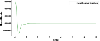
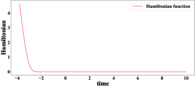
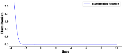
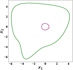
From (4.1), the approximate stable manifold is made up by all curves of solutions , . To construct the optimal controller, we need to find numerical solutions with Hamiltonian value under certain error tolerance. Projection of the approximate stable manifold (i.e. all extended curves) under certain error tolerance to -plane is a domain. In Figure 2, we illustrate the domains of projection of all extended curves with to -plane by the Störmer-Verlet method, RK45 and the method of Sakamoto-van der Schaft ([32, 31]) under certain error tolerances. It is clear that the Störmer-Verlet method generates a much larger domain comparing with the other two extension methods.
We should point out that, as shown above, the method of Sakamoto-van der Schaft ([32, 31]) requires much more iterative times, hence the computation cost is more expensive.
Remark 5.1.
We should mention that the Störmer-Verlet scheme is just a two order symplectic algorithm. If we need a larger domain, or a smaller Hamiltonian value tolerance is required, then other symplectic algorithms such as symplectic Runge-Kutta schemes of higher orders (see e.g. [16]) can be implemented.
5.2. Construct optimal controller by the approximate stable manifold
To find the approximate optimal controller by the stable manifold, we use the polynomial fitting method as in [31]. To be more precise, we first choose s according to the uniform distribution in . Using the computation procedure in Section 4.3 based on Störmer-Verlet scheme for time interval , and , we find extended curves in the stable manifold with the Hamiltonian less than . The projections of these curves to -plane belong to the domain (the largest domain in Figure 2). Then we select 10 points (including the point at time and the other 9 points chosen randomly in according to the uniform distribution) on each curve and the point . Hence we obtained a set of sample points on the stable manifold. To approximate stable manifold, we assume a polynomial fitting of form
where the coefficients are chosen by the least square technique based on the sample set . That is, are the coefficients to minimize
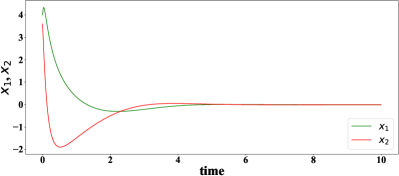
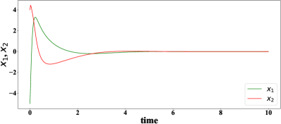
Then, using (2.3), the approximate optimal controller is given by . Hence by system (5.3), the closed loop can be computed for any . Here we demonstrate the controlled trajectories from the controller at some points in Figure 3. We can clearly see that the controller asymptotically stabilizes these trajectories.
6. Conclusion
In this note, using a symplectic algorithm for the stable manifolds of the Hamilton-Jacobi equations from infinite horizon optimal control, we construct a sequence of local approximate stable manifolds for Hamiltonian system at some hyperbolic equilibrium. In our approach, we first construct an iterative sequence of local approximate stable manifolds at equilibrium based on a precise estimates for the radius of convergence. Then, using symplectic algorithms, we enlarge the local approximate stable manifolds by solving initial value problem of the associated Hamiltonian system for . This avoids the divergent case of the iterative sequence as in [32] for unstable direction , and the computation cost can be reduced. Moreover, the symplectic algorithms have better long-time behaviours than general purpose numerical methods such as Runge-Kutta. The effectiveness of our algorithm is demostrated by an optimal control problem with exponential nonlinearity. Lastly, we should mention that the symplectic algorithm has potentials to be applied to more general Hamilton-Jacobi equations in control theory since such kind of equations have associated Hamiltonian systems as the characteristic systems.
.1. Proof of Theorem 3.1
Firstly, we prove that for ,
| (.1) |
where
| (.2) |
Here .
In fact, By Assumption 1, , Hence , . For , we prove by inductive method. Assume that the claim holds for . Then from (3) and (.1),
Let . Define , for . We should point out that the definition of is different from that in [32]. Note first that and . By mathematical induction, we can prove that and . Next solving
| (.5) |
Secondly, by a similar argument as in [32], we find that
| (.6) |
where and satisfy and , . Moreover, and are decreasing and , . Consequently, it holds that
| (.7) |
Thirdly, we prove that if , it holds that for all ,
| (.8) |
References
- [1] R. A. Abraham and J. E. Marsden. Foundation of mechanics. Benjamin/Cummings, Reading, MA, 2nd edition, 1978.
- [2] C. O. Aguilar and A. J. Krener. Numerical solutions to the Bellman equation of optimal control. Journal of Optimization Theory and Applications, 160(2):527–552, 2014.
- [3] E.G. Al’Brekht. On the optimal stabilization of nonlinear systems. Journal of Applied Mathematics and Mechanics, 25(5):1254–1266, 1961.
- [4] M. D. S. Aliyu. An approach for solving the Hamilton–Jacobi–Isaacs equation (HJIE) in nonlinear control. Automatica, 39(5):877–884, 2003.
- [5] M. D. S. Aliyu. A transformation approach for solving the Hamilton–Jacobi–Bellman equation in deterministic and stochastic optimal control of affine nonlinear systems. Automatica, 39(7):1243–1249, 2003.
- [6] J. A. Ball, J. W. Helton, and M. L. Walker. control for nonlinear systems with output feedback. IEEE Transactions on Automatic Control, 38(4):546–559, 1993.
- [7] R. W. Beard. Successive Galerkin approximation algorithms for nonlinear optimal and robust control. International Journal of Control, 71(5):717–743, 1998.
- [8] R. W. Beard, G. N. Saridis, and J. T. Wen. Galerkin approximations of the generalized Hamilton-Jacobi-Bellman equation. Automatica, 33(12):2159–2177, 1997.
- [9] S. C. Beeler, H. T. Tran, and H. T. Banks. Feedback control methodologies for nonlinear systems. Journal of Optimization Theory and Applications, 107(1):1–33, 2000.
- [10] S. Blanes and F. Casas. A concise introduction to geometric numerical integration. Chapman and Hall/CRC, 2016.
- [11] John R. Dormand and Peter J. Prince. A family of embedded Runge-Kutta formulae. Journal of computational and applied mathematics, 6(1):19–26, 1980.
- [12] E. Faou. Geometric numerical integration and Schrödinger equations, volume 15. European Mathematical Society, 2012.
- [13] K. Feng and M. Qin. Symplectic geometric algorithms for Hamiltonian systems. Springer, 2010.
- [14] L. Gauckler, E. Hairer, and C. Lubich. Dynamics, numerical analysis, and some geometry. Proceedings of the International Congress of Mathematicians (ICM 2018), pages 453–485, 2019.
- [15] E. Hairer, C. Lubich, and G. Wanner. Geometric numerical integration illustrated by the Störmer–Verlet method. Acta Numerica, 12:399–450, 2003.
- [16] E. Hairer, C. Lubich, and G. Wanner. Geometric numerical integration: structure-preserving algorithms for ordinary differential equations, volume 31. Springer Science & Business Media, 2006.
- [17] T. Horibe and N. Sakamoto. Nonlinear optimal control for swing up and stabilization of the acrobot via stable manifold approach: Theory and experiment. IEEE Transactions on Control Systems Technology, 27(6):2374–2387, Nov 2019.
- [18] T. Horibe and N. Sakamoto. Optimal swing up and stabilization control for inverted pendulum via stable manifold method. IEEE Transactions on Control Systems Technology, 26(2):708–715, 2017.
- [19] T. Hunt and A. J. Krener. Improved patchy solution to the Hamilton-Jacobi-Bellman equations. In 49th IEEE Conference on Decision and Control (CDC), pages 5835–5839. IEEE, 2010.
- [20] A. Isidori and A. Astolfi. Disturbance attenuation and -control via measurement feedback in nonlinear systems. IEEE Transactions on Automatic Control, 37(9):1283–1293, 1992.
- [21] G. Kreisselmeier and T. Birkholzer. Numerical nonlinear regulator design. IEEE Transactions on Automatic Control, 39(1):33–46, 1994.
- [22] P. Lancaster and L. Rodman. Algebraic Riccati equations. Clarendon press, 1995.
- [23] E. B. Lee and L. Markus. Foundations of Optimal Control Theory. New York: Wiley, 1967.
- [24] D. L. Lukes. Optimal regulation of nonlinear dynamical systems. SIAM Journal on Control, 7(1):75–100, 1969.
- [25] J. Markman and I. N. Katz. An iterative algorithm for solving Hamilton–Jacobi type equations. SIAM Journal on Scientific Computing, 22(1):312–329, 2000.
- [26] W. M. McEneaney. A curse-of-dimensionality-free numerical method for solution of certain HJB PDEs. SIAM Journal on Control and Optimization, 46(4):1239–1276, 2007.
- [27] C. P. Mracek and J. R. Cloutier. Control designs for the nonlinear benchmark problem via the state-dependent Riccati equation method. International Journal of Robust and Nonlinear Control, 8(4-5):401–433, 1998.
- [28] C. Navasca and A. J. Krener. Patchy solutions of Hamilton-Jacobi-Bellman partial differential equations. In Modeling, Estimation and Control, pages 251–270. Springer, 2007.
- [29] T. Ohtsuka. Solutions to the Hamilton-Jacobi equation with algebraic gradients. IEEE Transactions on Automatic Control, 56(8):1874–1885, 2010.
- [30] N. Sakamoto. Analysis of the Hamilton–Jacobi equation in nonlinear control theory by symplectic geometry. SIAM Journal on Control and Optimization, 40(6):1924–1937, 2002.
- [31] N. Sakamoto. Case studies on the application of the stable manifold approach for nonlinear optimal control design. Automatica, 49(2):568–576, 2013.
- [32] N. Sakamoto and A. J. van der Schaft. Analytical approximation methods for the stabilizing solution of the Hamilton–Jacobi equation. IEEE Transactions on Automatic Control, 53(10):2335–2350, 2008.
- [33] J. M. Sanz-Serna. Symplectic integrators for Hamiltonian problems: an overview. Acta numerica, 1:243–286, 1992.
- [34] J. M. Sanz-Serna and M.-P. Calvo. Numerical Hamiltonian problems. Courier Dover Publications, 2018.
- [35] Lawrence F. Shampine. Some practical Runge-Kutta formulas. Mathematics of Computation, 46: 135–150, 1986.
- [36] Y. B. Suris. The problem of integrable discretization: Hamiltonian approach, volume 219. Birkhäuser, 2012.
- [37] A. J. van der Schaft. On a state space approach to nonlinear control. Systems & Control Letters, 16(1):1–8, 1991.
- [38] A. J. van der Schaft. -gain analysis of nonlinear systems and nonlinear state feedback control. IEEE Transactions on Automatic Control, 37(6):770–784, 1992.