Symmetry-protected topological phases and competing orders
in a spin- XXZ ladder with a four-spin interaction
Abstract
We study a spin- XXZ model with a four-spin interaction on a two-leg ladder. By means of effective field theory and matrix product state calculations, we obtain rich ground-state phase diagrams that consist of eight distinct gapped phases. Four of them exhibit spontaneous symmetry breaking with either a magnetic or valence-bond-solid (VBS) long-range order. The other four are featureless, i.e., the bulk ground state is unique and does not break any symmetry. The featureless phases include the rung singlet (RS) and Haldane phases as well as their variants, the RS* and Haldane* phases, in which twisted singlet pairs are formed between the two legs. We argue and demonstrate that Gaussian transitions with the central charge occur between the featureless phases and between the ordered phases while Ising transitions with occur between the featureless and ordered phases. The two types of transition lines cross at the SU-symmetric point, where the criticality is described by the SU Wess-Zumino-Witten theory with . The RS-Haldane* and RS*-Haldane transitions give examples of topological phase transitions. Interestingly, the RS* and Haldane* phases, which have highly anisotropic nature, appear even in the vicinity of the isotropic case. We demonstrate that all the four featureless phases are distinguished by topological indices in the presence of certain symmetries.
I Introduction
The concept of symmetry-protected topological (SPT) phases has been proposed and fruitfully developed over the last decade [1, 2, 3, 4, 5, 6]. A SPT phase is a featureless gapped phase that does not exhibit spontaneous symmetry breaking but is distinguished from a trivial phase (i.e. a phase that includes a site-factorized product state) as long as certain symmetries are imposed. For example, Haldane phases [7, 8, 9] of odd-integer-spin chains are distinguished from trivial phases in the presence of the discrete spin rotation symmetry , time-reversal symmetry, or bond-centered inversion symmetry [1, 10, 11, 12, 13]. The Haldane phases with odd integer spins have been characterized by a string order parameter [14], hidden symmetry breaking [15, 16], a twist operator [17, 18], degeneracy in the edge states [19], the entanglement spectrum [10], and topological indices [10, 20, 21, 22]. Classification of SPT phases of bosons has been achieved by using the projective representations of the symmetry group in one dimension [21, 22, 23] and group cohomology theory in higher dimensions [24, 25].


A simple extension of the spin- Haldane phase can be found in a spin- two-leg ladder. Consider a spin- ladder with Heisenberg interactions and along the legs and rungs, respectively, where is assumed to be antiferromagnetic; see Fig. 1. Field-theoretical analyses indicate that the presence of the rung interaction immediately leads to gapped phases whose properties depend on the sign of [26, 27, 28]. In the gapped phase for ferromagnetic , effective spin- degrees of freedom emerge on the rungs and collectively form the Haldane state. This state can equivalently be viewed as a superposition of various singlet-covering states on a ladder. In contrast, the gapped phase for antiferromagnetic can be understood from the limit , where the ground state is a product state of singlet pairs on the rungs, known as the rung singlet (RS) state. The gapped phases for and are thus called the Haldane and RS phases, respectively. These phases are distinguished in terms of two types of string order parameters [29, 30, 31, 32] [shown in Eq. (5) later].
Liu et al. [33] have conducted a detailed classification of SPT phases in a spin- two-leg ladder for the symmetry group , where is the symmetry with respect to the interchange of the two legs. They have found three new SPT phases termed , all of which have symmetry-protected two-fold degenerate edge states on each end of an open ladder, with unique responses to magnetic fields. For example, the edge states in the phase are split by the magnetic field along the direction, but not by the fields in the and directions. The phase is related with the Haldane phase (termed in Ref. [33]) under the rotation of spins about the -axis on the first leg, , which provides some intuition on the ground state. Specifically, a singlet pair between spins on different legs turns into a twisted singlet under . It has also been argued that the trivial phase (i.e., the phase that includes rung-factorized states) is divided into four phases, termed rung- and rung-, if the translational symmetry is further imposed. The rung- phase corresponds to the conventional RS phase, and the rung- phase is obtained by operating the unitary transformation on the rung- phase. A highly anisotropic XYZ model on a ladder has been studied, which exhibits competition among the , , rung-, and rung- phases and a variety of magnetic phases (see also Ref. [34] and Appendix A). Fuji has given a field-theoretical description of a variety of SPT and symmetry-broken phases of a spin- XXZ ladder [35, 36]. Following him, we henceforth use the terms, the Haldane* and RS* phases, to refer to the and rung- phases, respectively, where a star indicates the operation of or equivalently the twist of singlet pairs between the legs. As the study of these phases has so far been limited in literature, it is worthwhile to further investigate when these phases emerge and how they compete with other phases in concrete spin models.
In this paper, we study a simple extension of the spin- Heisenberg ladder that has XXZ anisotropy and a four-spin interaction (Fig. 1). The Hamiltonian of our model is given by
| (1) |
where
| (2) |
The four-spin interaction with () introduces effective repulsion (attraction) between singlet pairs on the upper and lower edges of each plaquette. Throughout this paper, we take the leg interaction as the unit of energy. In contrast to the highly anisotropic models studied in Refs. [33, 34, 35], we investigate a regime around the isotropic case . By means of effective field theory for , we obtain rich ground-state phase diagrams that consist of eight distinct gapped phases, as schematically shown in Figs. 2 and 3. We also perform numerical calculations based on the variational uniform matrix product state (VUMPS) algorithm [37, 38] for to demonstrate that essentially the same phase structures continue for , as shown in Figs. 4 and 10 later. A notable feature as compared to Refs. [33, 34] is that the four featureless phases, i.e., the RS, RS*, Haldane, and Haldane* phases compete not only with magnetic phases but also with staggered dimer (SD) and columnar dimer (CD) phases, which have valence bond solid (VBS) long-range orders breaking the translational symmetry. It is also remarkable that the RS* and Haldane* phases, which have highly anisotropic wave functions involving twisted singlet pairs, appear even in the vicinity of the isotropic case . Below we briefly review previous studies on the model (I) and highlight our contributions.
The model (I) has been studied intensively in the isotropic case [39, 40, 41, 42, 43, 44, 45], which corresponds to the horizontal axes of Figs. 2 and 3. The SD and CD phases can be interpreted as a consequence of effective repulsion or attraction between singlet pairs due to . These phases have two-fold degenerate ground states below an excitation gap and are characterized by the order parameters
| (3a) | ||||
| (3b) | ||||
The translational symmetry as well as a symmetry with respect to the rung-centered reflection () are spontaneously broken in these phases. Field-theoretical analyses for weak inter-chain couplings () [39, 46, 44, 45] suggest that the RS-SD and Haldane-CD transitions are continuous and described by the SU Wess-Zumino-Witten (WZW) theory with the central charge , although a possibility of a first-order transition is not excluded. In this approach, the transition points are estimated to be for both signs of for [44]. More detailed phase diagrams on the - plane have been obtained numerically [42, 43, 45]. In particular, the exact diagonalization result of Ref. [42] for the RS-SD transition is consistent with the criticality for .
We have started our analysis of the anisotropic case in Ref. [47], and we extend it substantially in the present work. The obtained phase diagrams in Figs. 2 and 3 look like mirror images of each other 111 A useful way to relate the phases in Figs. 2 and 3 is to shift the lower leg of the ladder by one lattice spacing. In the bosonization formalism, this can be expressed as the shifts of and by and , respectively, as seen in Eq. (7). This corresponds to the shifts of and by and , respectively. The reason for this qualitative relation between Figs. 2 and 3 is as follows. In the bosonized expressions of spin and dimer operators in Eq. (7), the staggered components play a leading role. Therefore, an antiferromagnetic interaction on a rung, with , is qualitatively similar to a ferromagnetic interaction in a diagonal direction, , which is then transformed to a ferromagnetic interaction on a rung after the shift of the lower leg. A similar transformation can also be performed for . . The Haldane* and RS* phases, which are both featureless, appear for easy-plane anisotropy . The Néel and stripe Néel (SN) phases, which have magnetic long-range orders along the -axis, appear for easy-axis anisotropy . The Néel and SN phases have two-fold degenerate ground states below an excitation gap, and are characterized by the order parameters
| (4a) | ||||
| (4b) | ||||
A symmetry with respect to the global rotation of spins about the -axis ( and ) is spontaneously broken in these phases.
Our previous work [47] has focused on the nature of the phase transitions in the case of and easy-axis anisotropy , which corresponds to the upper half of Fig. 2. The Néel-SD transition is especially intriguing as it is between two ordered phases breaking different symmetries and may be viewed as a one-dimensional (1D) variant of deconfined quantum critical point [49, 50, 51, 52]. We have presented evidence that this transition belongs to the Gaussian universality class with . We have also demonstrated that the RS-Néel transition belongs to the Ising universality class with .
Our extended analysis in the present work demonstrates that the Gaussian and Ising transition lines found in Ref. [47] cross in the isotropic case and further continue to the easy-plane regime , as shown in Fig. 2. We also analyze the case of , and find similar crossing of the Gaussian and Ising transition lines, as shown in Fig. 3. In both the cases, the Gaussian transitions occur between featureless phases in the easy-plane regime , giving examples of topological phase transitions.
It is interesting to ask in what way the four featureless phases are distinguished. The following two types of string order parameters have been used to characterize the Haldane and RS phases [29, 30, 31, 32]:
| (5a) | ||||
| (5b) | ||||
Physically, these string order parameters detect the parity of the number of valence bonds cut by a vertical line between two adjacent rungs [32]. We obtain if is odd/even. Therefore, the Haldane and RS phases are characterized by non-vanishing of and for , respectively. As these order parameters remain unchanged under the operation of , the Haldane* and RS* phases are characterized similarly. However, these string order parameters do not distinguish between the Haldane and Haldane* phases or between the RS and RS* phases. We therefore calculate topological indices [10, 20, 21, 22] associated with and the translational symmetry, and demonstrate that these indices can distinguish all the four featureless phases.
The rest of this paper is organized as follows. In Sec. II, we present a field-theoretical analysis for weak inter-chain couplings, and derive the phase diagrams in Figs. 2 and 3. In Secs. III and IV, we present numerical results for and , respectively. In Sec. V, we analyze topological indices that distinguish the four featureless phases. In Sec. VI, we present a summary and an outlook for future studies. In Appendix A, we apply the field-theoretical formulation in Sec. II to an XYZ ladder studied by Liu et al. [33], and provide a qualitative description of their numerical results. In Appendices B and C, we provide some supplemental numerical results.
II Effective field theory
For weak inter-chain couplings with , the ground-state phase diagram of the model (I) can be studied by means of effective field theory based on bosonization [53, 54]. In our recent work [47], we have applied this formalism to study the case of and , i.e., the upper half of Fig. 2. Here we present a more detailed analysis that reveals the rich phase diagrams in Figs. 2 and 3. Our formulation is an extension of those in Refs. [26, 27, 28, 39, 44, 45, 46], and we take similar notations as those in Refs. [44, 47].
II.1 Bosonization
Here we briefly describe the bosonization formulation to obtain the low-energy effective Hamiltonian of the model (I) for . While this formulation has also been described in our previous paper [47], we summarize it for the purposes of selfcontainedness and fixing our notations.
We start from the two decoupled XXZ chains obtained for . Each chain labeled by is described effectively by the quantum sine-Gordon Hamiltonian
| (6) |
where and are a dual pair of bosonic fields. The Gaussian part of Eq. (6) is known as the Tomonaga-Luttinger liquid (TLL) theory and characterized by the spin velocity and the TLL parameter . The TLL parameter monotonically decreases as a function of , reaching at . When exceeds unity, the term with the scaling dimension becomes relevant (i.e., ) in the renormalization group (RG) sense, and induces the Néel order in the direction in each isolated chain. However, once the inter-chain couplings and are introduced, these couplings have much more significant impact on the low-energy physics than the term as we discuss later.
The spin and dimer operators on each chain are related to the bosonic fields as
| (7a) | |||
| (7b) | |||
| (7c) | |||
| (7d) | |||
where , is the lattice constant, and , , , , and are non-universal coefficients [55, 56, 44, 57]. At , these coefficients satisfy and because of the SU symmetry.
Treating and perturbatively and expressing them using Eq. (7), we obtain the low-energy effective Hamiltonian of the model (I) as
| (8) |
where and are symmetric and antisymmetric combinations of the bosonic fields and
| (9) |
with . The velocities and the TLL parameters in the symmetric and antisymmetric channels are in general modified from and in the decoupled XXZ chains by the effects of the inter-chain couplings. In Eq. (8), we focused on the most important terms around the isotropic case . Indeed, the and terms have the scaling dimensions and , respectively, which are all equal to unity in the limit of the decoupled Heisenberg chains. These terms are much more relevant than the term with the scaling dimension in Eq. (6). Therefore, the term can be ignored unless the anisotropy is significantly larger than and .
II.2 Expected phase diagrams
The symmetric and antisymmetric channels are separated in the effective Hamiltonian (8). The symmetric channel is described by the sine-Gordon model, in which the strongly relevant term locks at distinct positions depending on the sign of . A Gaussian transition with the central charge is expected at . The antisymmetric channel is described by the dual-field double sine-Gordon model, in which the strongly relevant and terms compete. When , in particular, both the terms have the same scaling dimensions of unity, and the long-distance physics can be determined by examining which of and is larger (in this case, the model is known as the self-dual sine-Gordon model [58]). Namely, () leads to the locking of (). Based on a mapping to Majorana fields, an Ising transition with the central charge has been shown to occur at [28, 58]. When deviates slightly from , a similar picture is still expected to hold as the change in is a marginal perturbation.
Based on this argument and the coupling constants in Eq. (9), we obtain the schematic phase diagrams around the isotropic case as shown in Figs. 2 and 3. Each phase is characterized by the locking positions of the bosonic fields. Remarkably, all the eight possible types of field locking in the effective Hamiltonian (8) occur in the two diagrams. In both the diagrams, a Gaussian transition in the symmetric channel occurs at (red line) while an Ising transition in the antisymmetric channel occurs at (blue line). The two transition lines cross at in the isotropic case , where the central charge is expected to be [42, 44, 43, 39, 45, 59, 46]; this point was estimated to be [44]. Below we discuss the phases appearing in these diagrams.
There are four ordered phases, the Néel, SN, SD, and CD phases. Using Eq. (7), we can express the order operators in Eqs. (3) and (4) in terms of the bosonic fields as
| (10a) | ||||
| (10b) | ||||
| (10c) | ||||
| (10d) | ||||
We can easily see that these operators acquire finite expectation values in the corresponding phases. For example, in the CD phase with in Fig. 3, we have , where is a constant independent of .
There are also four featureless phases, the RS, RS*, Haldane, and Haldane* phases. In these phases, the expectation values of all the operators in Eq. (10) vanish as fluctuates entirely owing to the locking of . These phases are instead characterized by the two types of string correlations in Eq. (5), which have the following bosonized expressions [60]:
| (11a) | ||||
| (11b) | ||||
We note that only the field in the symmetric channel is involved in these correlations. The Haldane and Haldane* phases with the field locking around exhibit non-vanishing values of for . Similarly, the RS and RS* phases with the field locking around 222While the RS and RS* phases have the field locking around and , respectively, in Figs. 2 and 3, these locking positions are equivalent. This is because the field on each leg is compactified as . exhibit non-vanishing for .
The difference between the Haldane and Haldane* phases or between the RS and RS* phases resides in the locking positions of , which cannot be detected by the string correlations (11). In fact, this difference can be used to show that the two phases are related by the unitary transformation [35]. Indeed, under this transformation, the field is shifted by as seen in Eq. (7b), and then the field is also shifted by . Identification of the Haldane* and RS* phases in the bosonization approach is based on this observation.
We have so far neglected possible perturbations to the effective Hamiltonian (8) which have larger scaling dimensions than the and terms. If such perturbations also become relevant, they can potentially change the nature of the phase transitions. In Ref. [47], we have addressed this issue for the case of the Néel-SD transition. Since the antisymmetric channel remains gapped at this transition, we can focus on the symmetric channel. As a possible perturbation, we can consider, for example, a higher-frequency cosine potential with the scaling dimension , which may lead to a first-order phase transition [62]. We have numerically demonstrated that stays around along the Néel-SD transition line in the parameter range investigated, and thus the above higher-frequency cosine term is likely to remain sufficiently irrelevant. As we have in the limit of decoupled Heisenberg chains, we can expect that our picture based on the leading terms in the effective Hamiltonian (8) would hold at least for weak inter-chain couplings.
II.3 Correlation functions around the Gaussian transitions
We have argued that Gaussian transitions occur between the ordered phases and between the featureless phases. We discuss the behavior of correlation functions around the presumed Gaussian transitions. As the case of the Néel-SD transition has been discussed previously [47], we focus on the other cases.
The SN-CD transition can be studied in a similar manner as the Néel-SD transition. We consider the following correlation functions
| (12a) | ||||
| (12b) | ||||
Each of these correlation functions would show a long-range order (i.e., convergence to a non-vanishing value for ) in the concerned phase and an exponential decay in the other phase. At the Gaussian transition, both of these functions would show a critical power-law decay. This can be shown in the following way. As seen in the bosonized expressions in Eq. (10), the operators and involve both the fields . As the symmetric channel is described by the Gaussian theory at the transition point, the symmetric component or shows a critical correlation with the decay exponent . In contrast, as remains locked around , the antisymmetric component shows a correlation that converges to a non-vanishing constant above the length scale proportional to the inverse of the excitation gap. Therefore, above this scale, the correlation functions in total exhibit the power-law behavior . In numerical calculations, the transition can be identified by plotting the two correlation functions in logarithmic scales and finding the point at which they both become linear and parallel to each other. We conduct this analysis in Sec. IV.2.
Next we consider the RS-Haldane* and RS*-Haldane transitions. We consider the two types of string correlation functions (5). Based on the bosonized expressions (11) and field locking positions in Figs. 2 and 3, we find that changes from an exponential decay to a long-range order across these transitions while changes in the opposite way. At the transition point, where the symmetric channel is described by the Gaussian theory, we have . Again, in numerical calculations, the transition point can be identified by linear and parallel behavior of the two correlation functions plotted in logarithmic scales. We conduct this analysis in Secs. III.1 and IV.1.
III Numerical results for
We have performed numerical calculations directly for the infinite system by applying the VUMPS algorithm [37, 38]. In this algorithm, a variational state is prepared in the form of a uniform matrix product state (MPS), and the ground state is obtained by iteratively optimizing constituent tensors to lower the variational energy. In applying it to the present ladder system, we regard two sites on each rung as a single effective site with the local Hilbert space dimension of four. In this section and the next, we adopt the two-site unit cell implementation in Ref. [37] as all the phases discussed in Sec. II have the unit cell consisting of at most two effective sites (i.e., two rungs). To ensure the sufficient convergence, we only used the data points that have the gradient norm , where is the gradient of energy per site with respect to the elementary tensor in VUMPS. The same method was employed in our previous work [47].
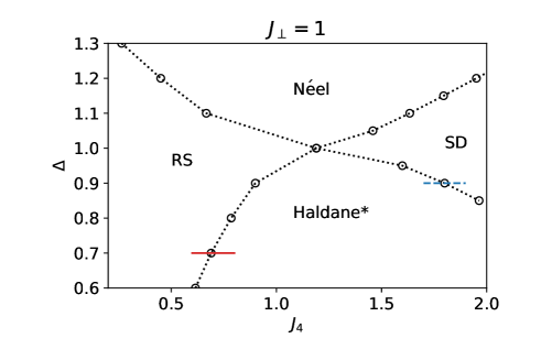
In this section, we fix and study the ground-state phase diagram in the - plane. The obtained phase diagram is shown in Fig. 4, which is qualitatively consistent with the field-theoretical prediction in Fig. 2. As the case of has been analyzed previously [42, 47], we focus on the easy-plane regime throughout this section. Below we explain how the RS-Haldane*-SD phase boundaries are obtained and how the critical properties at these transitions are characterized in our numerical analysis.
III.1 RS-Haldane* transition


Here we focus on the RS-Haldane* transition along the red solid line with in Fig. 4. In our VUMPS calculations, the ground state is obtained in the form of a period-2 MPS with the finite bond dimension . We can extract the correlation length from it in the following way. Let be the matrix for the state at the -th effective site. Using the matrices at the two neighboring sites and , we construct the combined matrix for the combined state . The correlation length is then calculated as , where is the second largest absolute eigenvalue of the transfer matrix . The obtained correlation length is plotted for different bond dimensions in Fig. 5. It shows a peak that grows consistently with an increase in , and the peak value exceeds lattice spacings for . However, the peaks in Fig. 5 are not as sharp as those found for the Néel-SD transition in Ref. [47]. Therefore, while Fig. 5 suggests the occurrence of a phase transition, it does not allow a precise determination of the RS-Haldane* transition point. We note that the non-sharpness of peaks has also been found for the RS-SD transition in the isotropic case [47], and is likely to be due to nontrivial effects of finite on transitions between valence bond phases. The transition point can instead be determined with reasonable accuracy through the analysis of the string correlations, which is done next.
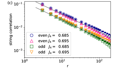
Figure 6 shows the numerical results on the two types of string correlation functions in Eq. (5). We find a qualitative difference between the ranges of and . For , is non-decaying at long distances while shows a rapid decay. For , is non-decaying while shows a rapid decay. These results are consistent with the occurrence of the RS-Haldane* transition. However, we note that (non-)decaying behavior of the two correlations only reflects the locking position of the field [see Eq. (11)], and that more detailed characterization of the phases requires the use of topological indices, which is done in Sec. V.
As discussed in Sec. II.3, the two string correlation functions show a power-law decay with the same exponent at the transition if it belongs to the Gaussian universality class. Therefore, the transition point can be identified by linear and parallel behavior of the two correlations plotted in logarithmic scales. As seen in Fig. 6(c), this should occur between and , giving the estimate of the transition point.
Critical points of a large class of 1D quantum systems are described by the conformal field theory (CFT). To investigate the underlying CFT, we calculate the entanglement entropy for a bipartition of the infinite 1D system into two half-infinite chains. According to the CFT, the entanglement entropy and the correlation length obey the scaling
| (13) |
where is the central charge and is a constant [63, 64]. The numerical results in Fig. 7 show a good agreement with this scaling with . Our results in Figs. 6(c) and 7 thus support the scenario that the RS-Haldane* transition belongs to the Gaussian universality class with .
III.2 Haldane*-SD transition
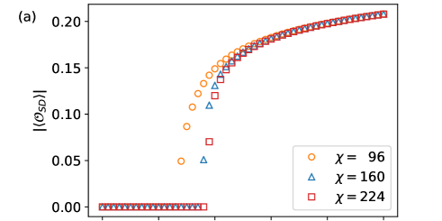


Here we focus on the Haldane*-SD transition along the blue dashed line with in Fig. 4. Figure 8(a) shows the SD order parameter , which indicates the onset of the SD order at a certain transition point . According to the effective field theory, the Haldane*-SD transition belongs to the Ising universality class with . In this universality class, the critical exponent for the spontaneous order parameter is given by . Therefore, it is expected that the order parameter to the eighth power becomes linear around the transition point and its intersect with the horizontal axis gives the estimate of the transition point. This analysis is performed in Fig. 8(b). We indeed find a good agreement with linear behavior in the range where the dependence on is sufficiently converged. The transition point is estimated to be .
IV Numerical results for

In this section, we fix and . The obtained phase diagram in Fig. 10 is qualitatively consistent with the field-theoretical prediction in Fig. 3. Below we explain how the phase boundaries are obtained and how the critical properties are characterized in our numerical analysis.
IV.1 RS*-Haldane transition


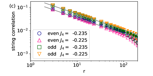
The RS*-Haldane transition can be analyzed in a similar manner as the RS-Haldane* transition discussed in Sec. III.1. Figure 11 shows the string correlation functions around the RS*-Haldane transition for . For , is non-decaying at long distances while shows a rapid decay. For , is non-decaying while shows a rapid decay. These results are consistent with the occurrence of the RS*-Haldane transition. More detailed characterization of these phases is given in terms of topological indices in Sec. V. Assuming the Gaussian universality class, the transition point can be identified by linear and parallel behavior of the two correlation functions plotted in logarithmic scales. This should occur between the two points examined in Fig. 11(c), giving the estimate . We have also confirmed the consistency with the central charge in a similar manner as in Fig. 7 (not shown).
IV.2 CD-SN transition


Figure 12 shows the CD and SN correlation functions (12) around the CD-SN transition for in Fig. 10. The data show the tendency of the CD and SN long-range orders for and , respectively. As discussed in Sec. II.3, the two correlation functions show a power-law decay with the same exponent at the transition point if the transition belongs to the Gaussian universality class. This should occur between the two points examined in Fig. 12(c), giving the estimate .
IV.3 Haldane-SN transition


The Haldane-SN transition can be analyzed in a similar manner as the Haldane*-SD transition discussed in Sec. III.2. Here, we fix and vary . Figure 13 shows our result on the SN order parameter . In the Ising universality class, is expected to be linear around the transition point . By performing the linear fitting of the data of versus and finding the intersect with the horizontal axis, we obtain the estimate . We also confirmed the consistency with the central charge in a similar manner as in Fig. 9 (not shown).
IV.4 RS*-CD transition

The RS*-CD transition can also be analyzed similarly. Here we fix , and plot the CD order parameter to the eighth power, , as a function of in Fig. 14. The numerical data show a rather significant dependence on the bond dimension . This behavior is specific to the RS*-CD transition, and is likely to be caused by its proximity to the CD-SN transition. We therefore perform the linear fitting individually for each bond dimension , find its intersect with the horizontal axis, and obtain the -dependent pseudo-critical point .

We extrapolate the pseudo-critical point to infinite by using the finite-bond-dimensional scaling. Finite-size scaling predicts that the true critical point and the pseudo-critical point satisfy
| (14) |
We assume that Eq. (14) holds by replacing the system size with the correlation length :
| (15) |
We also assume the Ising universality class with . Using this scaling, we obtain the critical point as shown in the inset in Fig. 14. Around the estimated critical point, we have confirmed the consistency with by examining the entanglement entropy versus the correlation length as shown in Fig. 15.
V Topological distinction among the four featureless phases
In the preceding sections, we have used two types of string correlations (5) in analyzing the RS-Haldane* and RS*-Haldane transitions. However, these correlations cannot be used to distinguish between the RS and RS* phases or between the Haldane and Haldane* phases. In this section, we demonstrate that topological indices [10, 20, 21, 22] associated with the symmetry and the translational symmetry can distinguish all the four featureless phases. Below we briefly review the basic formalism for classifying 1D SPT phases and calculating topological indices (especially, those of Pollmann and Turner [20]), and then apply it to the present ladder system. While the full classification of SPT phases in a spin- ladder with the symmetry has been achieved by Liu et al. [33], our results illustrate how those phases are identified unambiguously in numerical calculations.


Classification of 1D SPT phases can conveniently be discussed using the MPS representation [10, 11, 21, 22, 23]. Assuming the translational invariance, we represent the (normalized) ground state of the infinite system in the form of a canonical MPS as
| (16) |
Here, is a -by- matrix with being the spin state at a site, and is a diagonal matrix comprised of the Schmidt values associated with a bipartition of the system into half-infinite chains. In our application to the spin- ladder, runs over the four spin states on a rung. Suppose that is invariant under an on-site unitary transformation, which is represented in the spin basis as a unitary matrix acting on every site. Namely, we have , where is the state after the transformation. Then the matrices can be shown to satisfy [65]
| (17) |
where is a phase factor and is a -by- unitary matrix which commutes with . The phase factors form a 1D representation of the symmetry group. The matrices form a -dimensional projective representation of the symmetry group. Namely, it may differ from the linear representation by phase factors:
| (18) |
The phases , called the factor set of the representation, can be used to classify different phases. Specifically, if these phases cannot be gauged away by redefining the phases of , the state belongs to a nontrivial SPT phase. When the translational symmetry is further imposed, can also be used to classify phases [22].
To obtain the matrix and the phase factor numerically, we introduce a generalized transfer matrix
| (19) |
Let be the right eigenvector with the largest absolute eigenvalue :
| (20) |
where is normalized such that . Since we assumed , must have unit modulus. Conversely, if , we have . We now regard the vector with elements as a -by- matrix. One can show that if , and are equal to and , respectively, specifically, [20, 65].
We now focus on the case of a spin- ladder with the symmetry studied by Liu et al. [33]. The symmetry transformations acting on each rung are given by the spin rotations and and the inter-chain exchange . For these transformations, we can introduce the unitary matrices , , and and the corresponding indices , , and as explained above. While , , and commute with one another, the commutation relations among , , and may involve nontrivial phase factors. Such phase factors can be used as fingerprints of different phases. They can conveniently be detected by introducing traced commutators [20]
| (21) |
and
| (22) |
As explained above, we have if the state is not invariant under the transformation ; in this case, is zero by definition.
The commutation relations among , , and can be read off from Table I in Ref. [33], in which possible projective representations of and the corresponding SPT phases are summarized. If we do not impose the translational symmetry, the RS and RS* phases (termed rung- and rung- in Ref. [33]) fall into the trivial phase as they both include rung-factorized product states. In this trivial phase, , , and commute with one another, indicating . In contrast, the Haldane and Haldane* phases (termed and in Ref. [33]) show the nontrivial relation , indicating . Furthermore, the Haldane* phase shows , indicating . If we further impose the translational symmetry, the RS and RS* phases can be distinguished by the index . Indeed, by multiplying to a singlet and a twisted singlet on a rung, we find and in the RS and RS* phases, respectively. Therefore, we can distinguish the four featureless phases by using the indices , , and .
We have numerically calculated these topological indices in our model. Here, we have implemented the VUMPS algorithm not for multi-site unit cells as used in the previous sections but for single-site unit cells. With this implementation, transitions between featureless phases can be investigated more accurately; furthermore, the translational invariance is explicitly imposed, which is useful in applying the formalism described above. The procedure goes as follows. First, we calculate the ground state represented in a mixed canonical form. Second, we recast the state into a canonical form. Third, we construct the generalized transfer matrix (19), and obtain the largest eigenvalue and the corresponding right eigenvector , where the latter is equal to if . Finally, we calculate the traced commutators in Eqs. (21) and (22). Additionally, we have calculated the entanglement spectrum , which exhibits nontrivial degeneracy when some of ’s are noncommutative [10]. For example, when as in the Haldane and Haldane* phases, the entire spectrum shows double degeneracy as commutes with and .
Numerical results obtained around the RS-Haldane* and Haldane*-RS transitions are shown in Figs. 16 and 17, respectively. The numerical values of the indices , , and shown in the upper panels are in perfect agreement with the expected values in the four phases. The entanglement spectra shown in the lower panels show the expected double degeneracy in the Haldane and Haldane* phases. Physically, the double degeneracy arises if an odd number of (twisted) valence bonds are cut when the ladder is bipartitioned (see Appendix B for entanglement spectra in the ordered phases). In this sense, the degeneracy in the entanglement spectrum has similar information as the string correlation ; it cannot distinguish between the Haldane and Haldane* phases. Yet, more detailed information provided by the topological indices can distinguish all the four featureless phases.
VI Summary and outlook
In this paper, we have studied the spin- XXZ model with a four-spin interaction on a two-leg ladder in Eq. (I). By means of effective field theory and VUMPS calculations, we have obtained rich ground-state phase diagrams that consist of eight distinct gapped phases, as shown in Figs. 2, 3, 4, and 10. Notably, there are four featureless phases, i.e., the RS, RS*, Haldane, and Haldane* phases, which have a unique bulk ground state and do not break any symmetry. While the RS* and Haldane* phases have highly anisotropic nature, they are found to appear even in the vicinity of the isotropic case . In the obtained phase diagrams, the four featureless phases compete not only with magnetic phases but also with dimer phases that break the translational symmetry. We have argued and demonstrated that Gaussian transitions with the central charge occur between the featureless phases and between the ordered phases while Ising transitions with occur between the featureless and ordered phases. The two types of transition lines cross at the SU-symmetric point, where the criticality is described by the SU WZW theory with [39, 46, 43, 44, 45, 42]. As argued by Liu et al. [33], the four featureless phases are distinguished in the presence of the spin rotational dihedral symmetry , the inter-leg exchange symmetry , and the translational symmetry. We have demonstrated that these phases are indeed distinguished by topological indices associated with these symmetries.
An implication from the present work is that a rich phase structure can emerge by introducing anisotropy around the critical point described by the SU WZW theory. Such a structure has also been found in the spin- chain with bilinear and biquadratic interactions around the critical point known as the Takhtajan-Babujian model [66, 67, 68]: in the presence of uniaxial anisotropy , the Haldane, dimer, Néel, and large- phases compete around this point [69]. While the universality classes of the transitions among them have yet to be investigated, the phase structure is similar to Fig. 3. It would be interesting to extend this idea to other systems such as a generalized Hubbard ladder [59] and spin chains with higher symmetry [68]. Research along this direction may provide opportunities to explore further examples of SPT phases and to investigate their competition with ordered phases.


Acknowledgements.
The authors would like to thank Y. Fuji, R. K. Kaul, and M. Sato for useful comments. This research was supported by JSPS KAKENHI Grants No. JP18K03446, No. JP19H01809 and No. JP20K03780. The numerical computations were performed on computers at the Supercomputer Center, the Institute for Solid State Physics (ISSP), the University of Tokyo.Appendix A Effective field theory for a spin- XYZ ladder
In this appendix, we apply the field-theoretical formulation in Sec. II to a highly anisotropic XYZ model on a ladder described by the Hamiltonian
| (23) |
This model is equivalent to the model studied by Liu et al. [33], and our analysis gives a qualitative description of their numerical results, as we explain in the following.
We set and assume . Treating ’s perturbatively, we obtain the low-energy effective Hamiltonian similar to Eq. (8) but with the additional term . The coupling constants in this effective Hamiltonian are given by
| (24) |
Assuming that is close to unity, we can determine the ground-state phase diagram in a similar manner as in Sec. II.2.
We first consider the case of . In this case, the model (23) has the spin-rotational symmetry. Reflecting this symmetry, the term vanishes and a magnetic order is allowed only along the axis. The obtained phase diagram in Fig. 18 exhibits competition among four featureless phases and two phases with magnetic orders along the axis. This diagram agrees qualitatively with Fig. 5 in Ref. [33], which is for . In the latter figure, however, the RS-Haldane* and RS*-Haldane phase boundaries are largely bent downward with increasing ; this behavior is beyond the scope of the present analysis for weak inter-chain couplings. We refer the reader to Ref. [70] for a related bosonization analysis on a 1D anisotropic Kondo lattice.
We next consider the case of and . In this case, the model (23) does not have the spin-rotational symmetry. The obtained phase diagram in Fig. 19 exhibits competition among four featureless phases and four phases with magnetic orders along the or axis. In the limit , where , the Néelz and SNz phases disappear, and Fig. 19 should become equivalent to Fig. 18 although the roles of the and directions are interchanged. Figure 19 agrees qualitatively with Fig. 1 in Ref. [33], which is for , if we interchange the and directions. However, the latter figure indicates that the rung- and rung- phases are much broader and the and phases are much narrower than in Fig. 19. We note that our conditions for finding Ising transitions in the dual-field double sine-Gordon model are only approximate ones for and can become inaccurate even in the regime of weak inter-chain couplings as deviates from unity.
Finally, we note that although the coupling constants in Eq. (24) are subject to the constraint , this constraint can be released by adding the four-spin interaction , as seen in Eq. (9). By varying and in the regime of weak inter-chain couplings, one can fully control the signs and the relative magnitudes of and . This huge space allows one to obtain 16 possible phases: the rung-, rung-, , , Néelμ, SNμ (), SD, and CD phases.
Appendix B Entanglement spectra in the ordered phases

In Sec. V, we have calculated the entanglement spectra in the four featureless phases, as shown in Figs. 16 and 17. In this appendix, we discuss the entanglement spectra in the four ordered phases.
All the ordered phases discussed in the paper have the unit cell consisting of two effective sites (i.e., two rungs). We have therefore adopted the two-site unit cell implementation of the VUMPS algorithm as explained in Sec. III. Numerical results on the entanglement spectra are shown in Fig. 20. It is expected that the entire spectrum shows at least double degeneracy if an odd number of valence bonds are cut when bipartitioning the system [10]. The spectrum in the SD phase indeed shows the expected double degeneracy. In the CD phase, the spectra depend on where the system is cut. Specifically, we have obtained the CD state with [see Eq. (3b) for the definition of the order parameter]. The spectrum labeled “CD1” is for the case when the cut is placed between the st and th rungs. The spectrum labeled “CD2” is for the case when the cut is placed between the th and st rungs. The entanglement entropy is larger in the latter case. In an ideal CD state as shown in the inset in Fig. 3, two valence bonds are cut in the “CD2” case, leading to 4-fold degeneracy in the entanglement spectrum. However, this degeneracy is split in a generic CD state. Therefore, there is no symmetry-protected degeneracy in the entanglement spectrum in the CD phase. The Néel and SN phases do not exhibit any symmetry-protected degeneracy in the entanglement spectra, either, as they include site-factorized product states with no entanglement.
Appendix C Phase transitions in the isotropic case


In this appendix, we estimate the RS-SD and Haldane-CD transition points in the isotropic case . Field-theoretical analyses for weak inter-chain couplings () [39, 46, 44, 45] suggest that these transitions are continuous and described by the SU WZW theory with the central charge , although a possibility of a first-order transition is not excluded. The SU WZW theory is equivalent to the combination of the Gaussian theory with in the symmetric channel and the Ising CFT in the antisymmetric channel. In estimating the transition points, we use the two types of string correlation functions (5) as they can selectively probe the information in the symmetric channel as seen in Eq. (11). Specifically, these correlation functions are expected to show power-law decay with the same exponent at the transition if the scenario of the SU WZW theory is true.
Figure 21 shows the numerical result around the RS-SD transition at . The result indicates that a power-law decay of the two correlation functions with the same exponent is likely to occur between and . This result is consistent with the previous estimate of the transition point by exact diagonalization [42]. At this point, we have obtained the central charge by examining the data of the entanglement entropy versus the correlation length in our previous work [47]. Our results are thus consistent with the scenario of the SU WZW theory.
Figure 22 shows the numerical result around the CD-Haldane transition at . The result indicates that power-law decay with the same exponent can occur between and . We thus obtain the estimate of the transition point, which still has a relatively large error range. However, we have found that if we try to reduce the range of further, one of the two correlation functions becomes inconsistent with the behavior. This is likely to be due to insufficient convergence of the numerical data as a function of although the breakdown of the scenario of the SU WZW theory is not excluded. Our estimate of the transition point could be compared with the exact diagonalization result of Hijii and Sakai [43] (in particular, Figs. 5 and 6 therein). However, because of a relatively large dependence on the system size in Ref. [43], a detailed consistency check is not possible.
References
- Gu and Wen [2009] Z.-C. Gu and X.-G. Wen, Phys. Rev. B 80, 155131 (2009).
- Chen et al. [2010] X. Chen, Z.-C. Gu, and X.-G. Wen, Phys. Rev. B 82, 155138 (2010).
- Wen [2019] X.-G. Wen, Science 363, 10.1126/science.aal3099 (2019).
- Senthil [2015] T. Senthil, Annual Review of Condensed Matter Physics 6, 299 (2015).
- Zeng et al. [2019] B. Zeng, X. Chen, D.-L. Zhou, and X.-G. Wen, Quantum information meets quantum matter: from quantum entanglement to topological phases of many-body systems, Quantum science and technology (Springer, New York, NY, 2019).
- Tasaki [2020] H. Tasaki, Physics and mathematics of quantum many-body systems, Graduate texts in physics (Springer, 2020).
- Haldane [1983a] F. D. M. Haldane, Physics Letters A 93, 464 (1983a).
- Haldane [1983b] F. D. M. Haldane, Phys. Rev. Lett. 50, 1153 (1983b).
- Affleck [1989] I. Affleck, Journal of Physics: Condensed Matter 1, 3047 (1989).
- Pollmann et al. [2010] F. Pollmann, A. M. Turner, E. Berg, and M. Oshikawa, Phys. Rev. B 81, 064439 (2010).
- Pollmann et al. [2012] F. Pollmann, E. Berg, A. M. Turner, and M. Oshikawa, Phys. Rev. B 85, 075125 (2012).
- Ogata [2020] Y. Ogata, Communications in Mathematical Physics 374, 705 (2020).
- Ogata [2019] Y. Ogata, A -index of symmetry protected topological phases with reflection symmetry for quantum spin chains (2019), arXiv:1904.01669 [math-ph] .
- den Nijs and Rommelse [1989] M. den Nijs and K. Rommelse, Phys. Rev. B 40, 4709 (1989).
- Kennedy and Tasaki [1992] T. Kennedy and H. Tasaki, Phys. Rev. B 45, 304 (1992).
- Oshikawa [1992] M. Oshikawa, Journal of Physics: Condensed Matter 4, 7469 (1992).
- Nakamura and Todo [2002] M. Nakamura and S. Todo, Phys. Rev. Lett. 89, 077204 (2002).
- Tasaki [2018] H. Tasaki, Phys. Rev. Lett. 121, 140604 (2018).
- Kennedy [1990] T. Kennedy, Journal of Physics: Condensed Matter 2, 5737 (1990).
- Pollmann and Turner [2012] F. Pollmann and A. M. Turner, Phys. Rev. B 86, 125441 (2012).
- Chen et al. [2011a] X. Chen, Z.-C. Gu, and X.-G. Wen, Phys. Rev. B 83, 035107 (2011a).
- Chen et al. [2011b] X. Chen, Z.-C. Gu, and X.-G. Wen, Phys. Rev. B 84, 235128 (2011b).
- Schuch et al. [2011] N. Schuch, D. Pérez-García, and I. Cirac, Phys. Rev. B 84, 165139 (2011).
- Chen et al. [2012] X. Chen, Z.-C. Gu, Z.-X. Liu, and X.-G. Wen, Science 338, 1604 (2012).
- Chen et al. [2013] X. Chen, Z.-C. Gu, Z.-X. Liu, and X.-G. Wen, Phys. Rev. B 87, 155114 (2013).
- Strong and Millis [1992] S. P. Strong and A. J. Millis, Phys. Rev. Lett. 69, 2419 (1992).
- Strong and Millis [1994] S. P. Strong and A. J. Millis, Phys. Rev. B 50, 9911 (1994).
- Shelton et al. [1996] D. G. Shelton, A. A. Nersesyan, and A. M. Tsvelik, Phys. Rev. B 53, 8521 (1996).
- Watanabe et al. [1993] H. Watanabe, K. Nomura, and S. Takada, Journal of the Physical Society of Japan 62, 2845 (1993).
- Nishiyama et al. [1995] Y. Nishiyama, N. Hatano, and M. Suzuki, Journal of the Physical Society of Japan 64, 1967 (1995).
- Kim et al. [2000] E. H. Kim, G. Fáth, J. Sólyom, and D. J. Scalapino, Phys. Rev. B 62, 14965 (2000).
- Kim et al. [2008] E. H. Kim, O. Legeza, and J. Sólyom, Phys. Rev. B 77, 205121 (2008).
- Liu et al. [2012] Z.-X. Liu, Z.-B. Yang, Y.-J. Han, W. Yi, and X.-G. Wen, Phys. Rev. B 86, 195122 (2012).
- Manmana et al. [2013] S. R. Manmana, E. M. Stoudenmire, K. R. A. Hazzard, A. M. Rey, and A. V. Gorshkov, Phys. Rev. B 87, 081106 (2013).
- Fuji [2015] Y. Fuji, Symmetries and quantum phases in one-dimensional spin systems, Ph.D. thesis, University of Tokyo (2015).
- Fuji [2016] Y. Fuji, Phys. Rev. B 93, 104425 (2016).
- Zauner-Stauber et al. [2018] V. Zauner-Stauber, L. Vanderstraeten, M. T. Fishman, F. Verstraete, and J. Haegeman, Phys. Rev. B 97, 045145 (2018).
- Vanderstraeten et al. [2019] L. Vanderstraeten, J. Haegeman, and F. Verstraete, SciPost Phys. Lect. Notes , 7 (2019).
- Nersesyan and Tsvelik [1997] A. A. Nersesyan and A. M. Tsvelik, Phys. Rev. Lett. 78, 3939 (1997).
- Pati et al. [1998] S. K. Pati, R. R. P. Singh, and D. I. Khomskii, Phys. Rev. Lett. 81, 5406 (1998).
- Itoi et al. [2000] C. Itoi, S. Qin, and I. Affleck, Phys. Rev. B 61, 6747 (2000).
- Hijii and Nomura [2009] K. Hijii and K. Nomura, Phys. Rev. B 80, 014426 (2009).
- Hijii and Sakai [2013] K. Hijii and T. Sakai, Phys. Rev. B 88, 104403 (2013).
- Takayoshi and Sato [2010] S. Takayoshi and M. Sato, Phys. Rev. B 82, 214420 (2010).
- Robinson et al. [2019] N. J. Robinson, A. Altland, R. Egger, N. M. Gergs, W. Li, D. Schuricht, A. M. Tsvelik, A. Weichselbaum, and R. M. Konik, Phys. Rev. Lett. 122, 027201 (2019).
- Müller et al. [2002] M. Müller, T. Vekua, and H.-J. Mikeska, Phys. Rev. B 66, 134423 (2002).
- Ogino et al. [2021] T. Ogino, R. Kaneko, S. Morita, S. Furukawa, and N. Kawashima, Phys. Rev. B 103, 085117 (2021).
- Note [1] A useful way to relate the phases in Figs. 2 and 3 is to shift the lower leg of the ladder by one lattice spacing. In the bosonization formalism, this can be expressed as the shifts of and by and , respectively, as seen in Eq. (7\@@italiccorr). This corresponds to the shifts of and by and , respectively. The reason for this qualitative relation between Figs. 2 and 3 is as follows. In the bosonized expressions of spin and dimer operators in Eq. (7\@@italiccorr), the staggered components play a leading role. Therefore, an antiferromagnetic interaction on a rung, with , is qualitatively similar to a ferromagnetic interaction in a diagonal direction, , which is then transformed to a ferromagnetic interaction on a rung after the shift of the lower leg. A similar transformation can also be performed for .
- Senthil et al. [2004] T. Senthil, A. Vishwanath, L. Balents, S. Sachdev, and M. P. A. Fisher, Science 303, 1490 (2004), https://science.sciencemag.org/content/303/5663/1490.full.pdf .
- Jiang and Motrunich [2019] S. Jiang and O. Motrunich, Phys. Rev. B 99, 075103 (2019).
- Roberts et al. [2019] B. Roberts, S. Jiang, and O. I. Motrunich, Phys. Rev. B 99, 165143 (2019).
- Mudry et al. [2019] C. Mudry, A. Furusaki, T. Morimoto, and T. Hikihara, Phys. Rev. B 99, 205153 (2019).
- Giamarchi [2004] T. Giamarchi, Quantum Physics in One Dimension, International Series of Monographs on Physics (Oxford University Press, New York, 2004).
- Gogolin et al. [2004] A. Gogolin, A. Nersesyan, and A. Tsvelik, Bosonization and Strongly Correlated Systems (Cambridge University Press, New York, 2004).
- Lukyanov and Zamolodchikov [1997] S. Lukyanov and A. Zamolodchikov, Nuclear Physics B 493, 571 (1997).
- Hikihara and Furusaki [1998] T. Hikihara and A. Furusaki, Phys. Rev. B 58, R583 (1998).
- Hikihara et al. [2017] T. Hikihara, A. Furusaki, and S. Lukyanov, Phys. Rev. B 96, 134429 (2017).
- Lecheminant et al. [2002] P. Lecheminant, A. O. Gogolin, and A. A. Nersesyan, Nuclear Physics B 639, 502 (2002).
- Tsuchiizu and Furusaki [2002] M. Tsuchiizu and A. Furusaki, Phys. Rev. B 66, 245106 (2002).
- Nakamura [2003] M. Nakamura, Physica B: Condensed Matter 329-333, 1000 (2003), proceedings of the 23rd International Conference on Low Temperature Physics.
- Note [2] While the RS and RS* phases have the field locking around and , respectively, in Figs. 2 and 3, these locking positions are equivalent. This is because the field on each leg is compactified as .
- Furukawa et al. [2010] S. Furukawa, M. Sato, and A. Furusaki, Phys. Rev. B 81, 094430 (2010).
- Calabrese and Cardy [2004] P. Calabrese and J. Cardy, Journal of Statistical Mechanics: Theory and Experiment 2004, P06002 (2004).
- Pollmann et al. [2009] F. Pollmann, S. Mukerjee, A. M. Turner, and J. E. Moore, Phys. Rev. Lett. 102, 255701 (2009).
- Pérez-García et al. [2008] D. Pérez-García, M. M. Wolf, M. Sanz, F. Verstraete, and J. I. Cirac, Phys. Rev. Lett. 100, 167202 (2008).
- Takhtajan [1982] L. Takhtajan, Physics Letters A 87, 479 (1982).
- Babujian [1982] H. Babujian, Physics Letters A 90, 479 (1982).
- Affleck [1986] I. Affleck, Nuclear Physics B 265, 409 (1986).
- De Chiara et al. [2011] G. De Chiara, M. Lewenstein, and A. Sanpera, Phys. Rev. B 84, 054451 (2011).
- Nakagawa and Kawakami [2017] M. Nakagawa and N. Kawakami, Phys. Rev. B 96, 155133 (2017).