Symmetry Induces Structure and Constraint of Learning
Abstract
Due to common architecture designs, symmetries exist extensively in contemporary neural networks. In this work, we unveil the importance of the loss function symmetries in affecting, if not deciding, the learning behavior of machine learning models. We prove that every mirror-reflection symmetry, with reflection surface , in the loss function leads to the emergence of a constraint on the model parameters : . This constrained solution becomes satisfied when either the weight decay or gradient noise is large. Common instances of mirror symmetries in deep learning include rescaling, rotation, and permutation symmetry. As direct corollaries, we show that rescaling symmetry leads to sparsity, rotation symmetry leads to low rankness, and permutation symmetry leads to homogeneous ensembling. Then, we show that the theoretical framework can explain intriguing phenomena, such as the loss of plasticity and various collapse phenomena in neural networks, and suggest how symmetries can be used to design an elegant algorithm to enforce hard constraints in a differentiable way.
1 Introduction
Modern neural networks are so large that they contain an astronomical number of neurons and connections layered in a highly structured manner. This design of modern architectures and loss functions means that there are a lot of redundant parameters in the model and that the loss functions are often invariant to hidden, nonlinear, and nonperturbative transformations of the model parameters. We call these invariant transformations the “symmetries” of the loss function. Common examples of symmetries in the loss function include the permutation symmetry (Simsek et al., 2021; Entezari et al., 2021; Hou et al., 2019), rescaling symmetry (Dinh et al., 2017; Saxe et al., 2013; Neyshabur et al., 2014; Tibshirani, 2021), scale symmetry (Ioffe & Szegedy, 2015) and rotation symmetry (Ziyin et al., 2023b). In physics, symmetries are regarded as fundamental organizing principles of nature, and systems with symmetries exhibit rich and hierarchical behaviors (Anderson, 1972). However, existing works study specific symmetries case-by-case, and no unifying theory exists to understand the role of symmetries in affecting the learning of neural networks. In this work, we take a neutral stance and show that the common types of symmetries can be understood in a unified theoretical framework of what we call the “mirror symmetries”, where every symmetry is proved to lead to a special structure and constraint of optimization.
Since we will also discuss stochastic aspects of learning, we study a generic twice-differentiable non-negative per-sample loss function:
| (1) |
where is a minibatch or a single data point of arbitrary dimension and sampled from a training set. is the model parameter, and is the weight decay. assumes the definition of the model architecture and is the data-dependent part of the loss. Training with stochastic gradient descent (SGD), we sample a set of and compute the gradient of the averaged per-sample loss over the set. The per-sample loss averaged over the training set is the empirical risk: . Training with gradient descent (GD), we compute the gradient with respect to . All the results we derive for directly carry over to . Also, because the sampling over is equivalent to a sampling of , we omit from the equations unless necessary.
The main contributions are the following:
-
1.
we identify a general class of symmetry, the mirror reflection symmetry, that treats all common types of symmetry in a coherent framework;
-
2.
we prove that every mirror symmetry leads to a constraint on the parameters, and when weight decay is used (or when the gradient noise is large), SGD training tends to converge to these constrained symmetric solutions;
-
3.
we apply the theory to understand phenomena related to common symmetries such as rescaling, rotation symmetry, and permutation symmetry.
Experiments and discussions of previous results show that the theory is highly practically relevant. This work is organized as follows. We present the proposed theory and discuss its implications in depth in the next section. We apply the result to four different problems and numerically validate the theory in Section 3. We discuss the closely related works in Section 4. The last section concludes this work. All the proofs are given in Appendix C.

2 Mirror Symmetry Leads to Constraints
2.1 Main Theorem
Let us first define a general type of symmetry called mirror reflection symmetry.
Definition 1.
A per-sample loss function is said to have the simple mirror (reflection) symmetry with respect to a unit vector if, for all , .
Note that the vector is the reflection of with respect to the plane orthogonal to . Also, the regularization term itself satisfies this symmetry for any because reflection is norm-preserving. An important quantity is the average of the two reflected solutions: , where is the fixed point of this transformation and is called a “symmetric solution.” This mirror symmetry can be generalized to the case where the loss function is invariant only when multiple mirror reflections are made.
Definition 2.
Let consist of columns of orthonormal vectors: , and . A loss function is said to have the -mirror symmetry if, for all , .
By construction, and are projection matrices, and is an orthogonal matrix. There are a few equivalent ways to see this symmetry. First of all, it is equivalent to requiring the loss function to be invariant only after multiple simple mirror symmetry transformations. Let be a unit vector orthogonal to . Reflections to both and give . The matrix is a projection matrix and, thus, an instantiation of . Secondly, because the composition of orthogonal unit vectors spans the space of projection matrices, is nothing but a generic projection matrix . Thus, this symmetry can be equivalently defined with respect to such that . If we let or be rank-, the symmetry reduces to the simple mirror symmetry in Definition 1. We will see in Section 3 that many common types of symmetries in deep learning imply mirror symmetries.
We also make a reasonable smoothness assumption, which is only needed for part 4 of the theorem. This assumption is benign because any function satisfies this assumption in a bounded space.
Assumption 1.
The smallest eigenvalue of the Hessian of is lower-bounded by a (possibly negative) constant
With these definitions, we are ready to prove the following theorem.
Theorem 1.
Let satisfy the -mirror symmetry. Then,
-
1.
for any , if , then ;
-
2.
if , a subset of the eigenvector of spans , and the rest spans ;
-
3.
if , there exists such that for all , ;
-
4.
there exists such that for all , all minima of satisfy .
Parts 1 and 2 are statements regarding the local gradient geometry, regardless of the weight decay. Parts 3 and 4 are local and global statements regarding the role of weight decay, which points to a novel mechanism through which weight decay regularizes a neural network. The fact that the constrained solutions become local minima even at a finite weight decay means that weight decay favors a sparse solution (sparse in the subspace of symmetry breaking). This is different from the behavior of weight for linear regression, where the model only becomes sparse when the weight decay is infinite. Therefore, textbooks often say that regularization leads to a dense solution (Bishop & Nasrabadi, 2006; Hastie et al., 2009). The fact that sparse solutions are favored under weight decay is thus a unique feature of deep learning. See Figure 1 for an illustration of mirror symmetries and the intuition behind the proof. We will explain these parts of the theorem in depth below. Lastly, note that this theorem applies to arbitrary function that has the mirror symmetry, which does not need to be a loss function.


2.2 Absorbing States and Stationary Conditions
To discuss the implication of symmetries, we introduce the concept of a “stationary condition.”
Definition 3.
For an arbitrary function , is a stationary condition of if implies , where is the -th step parameter under (stochastic) gradient descent.
A stationary condition can be seen as a special case of an absorbing state, which is a major theme in the study of Markov processes and is associated with complex phase-transition-like behaviors (Norris, 1998; Dickman & Vidigal, 2002; Hinrichsen, 2000). Part 1 of Theorem 1 implies the following.
Corollary 1.
Every -mirror symmetry implies a linear stationary condition: .
Alternatively, a stationary condition can be seen as a generalization of a stationary point because every stationary point in the landscape implies the existence of a stationary condition – but not vice versa. For example, some functions of the parameters might reach stationarity before the whole model reaches stationarity. The existence of such conditions implies that there are special subspaces in the landscape such that the dynamics of (S)GD within these subspaces will not leave it. See Appendix Figure 5 for an illustration of the stationary conditions.
2.3 Structure of the Hessian
Part 2 of Theorem 1 has important implications for the local geometry of the loss and the dynamics of SGD. Let denote the Hessian of the loss or that of the per-sample loss . Part 2 states that close to symmetry solutions are partitioned by the symmetry condition to two subspaces: one part aligns with the images of , and the other part must be orthogonal to it. Namely, one can transform the Hessian into a two-block form, and , with .111Let be any orthogonal matrix whose basis includes all the eigenvectors of . Then, will be a two-block matrix. Note that the parameters might also contain other symmetries, so and may also consist of multiple sub-blocks. This implies that close to the symmetric solutions, the Hessian of the loss will take a highly structured form simultaneously for all data points or batches. See Figure 2.
The fact that the Hessian of neural networks takes a similar structure after training is supported by empirical works. For example, the illustrative Hessian in Figure 2 is similar to that computed in Sagun et al. (2016). That the actual Hessians after training are well approximated by smaller blocks is supported by Wu et al. (2020). Blockwise Hessian matrices can also be related to the existence of gaps in the Hessian spectrum, which is widely observed (Sagun et al., 2017; Ghorbani et al., 2019; Wu et al., 2020; Papyan, 2018).
It is instructive to consider the special case where is rank-. Part 2 implies that must be an eigenvector of the Hessian whenever the model is at a symmetry solution. For example, we consider a two-layer tanh network with scalar input and outputs. The loss function can always be written as . For each index , contains a symmetry with the identity mirror . Therefore, the theory predicts that when , the Hessian consists of block matrices. If we also recognize that a tanh network approximates a linear network at the origin, we see that there are actually two mirrors: and , which are the eigenvectors of the Hessian according to the theory. This can be compared with a direct computation. When , the nonvanishing terms of the Hessian are :
| (2) |
This means the Hessian is indeed -block and that the eigenvectors are and , agreeing with the theory. It is remarkable that we can identify all the eigenvectors of an arbitrarily wide nonlinear network by examining the symmetry in the model.
2.4 Dynamics of Stochastic Gradient Descent
The loss symmetry has a major implication for the dynamics of SGD. Because the Hessian is block-wise with fixed blocks (with probability 1), the dynamics of SGD in the symmetry direction and the symmetry-breaking direction are essentially independent. Let denote the mirror and the projection matrix. If where is a unit vector, and is a small quantity, the model is perturbatively away from the symmetry solution. In this case, one can expand the loss function to leading orders in :
| (3) |
where we have defined the sample Hessian restricted to the projected subspace: , which is a matrix of random variables. Note that all the odd-order terms in vanish due to the symmetry in flipping the sign of . In fact, one can view the training loss or as a function of , which we denote as , and this analysis implies that the loss landscape close to has a universal geometry. See Figure 2.
This allows us to characterize the dynamics of SGD in the symmetry directions:
| (4) |
where is the learning rate. If one model as a random matrix, this dynamics reduces to the classical problem of random matrix product (Furstenberg & Kesten, 1960). In general, the symmetric solutions at are saddle points, while the attractivity of only depends on the sign of Lyapunov exponent of dynamics. This implies that these types of saddles points are often attractive.
To compare, we first consider GD. The largest negative eigenvalue of , , thus gives the speed at which SGD escapes the stationary condition: . When weight decay is present, all the eigenvalues of will be positively shifted by , and, therefore, if and only if , GD will be attracted to these symmetric solutions. In this sense, gives a critical weight decay value at which a symmetry-induced constraint is favored.
For SGD, the dynamics is qualitatively different. The naive expectation is that, when using SGD, the model will escape the stationary condition faster due to the noise. However, this is the opposite of the truth. The existence of the SGD noise due to minibatch sampling makes these stationary conditions more attractive. The stability of the type of dynamics in Eq. (4) can be analyzed by studying the condition for convergence in probability of the solution (Ziyin et al., 2023a). One can show that converges to in probability if and only if the Lyapunov exponent of the process is negative, which is possible even if this critical point is a strict saddle. When does a subspace of converge (or collapse) to zero? A qualitatively correct critical learning rate can be derived using a diagonal approximation of the Hessian. In this case, each subspace of has its own Lyapunov exponent and can be analytically computed. Let denote the eigenvalue of in this subspace. Then, this subspace collapses when , which is negative for a large learning rate (see Appendix C for a formal treatment). The meaning of this condition becomes clear by expanding to the second order in to obtain:
| (5) |
The numerator is the eigenvalue of the empirical loss, and the denominator can be identified as the minibatch noise effect (Wu et al., 2018), which becomes larger if the batch size is small or if the dataset is noisy. Therefore, this phenomenon happens due to the competition between the signal and noise in the gradient. This example shows that at a large learning rate, the stationary conditions are favored solutions of SGD, even if they are not favored by GD. Also, convergence to these symmetry-induced saddles is not a unique feature of SGD but happens for Adam-type dynamics as well (Ziyin et al., 2021, 2023a).
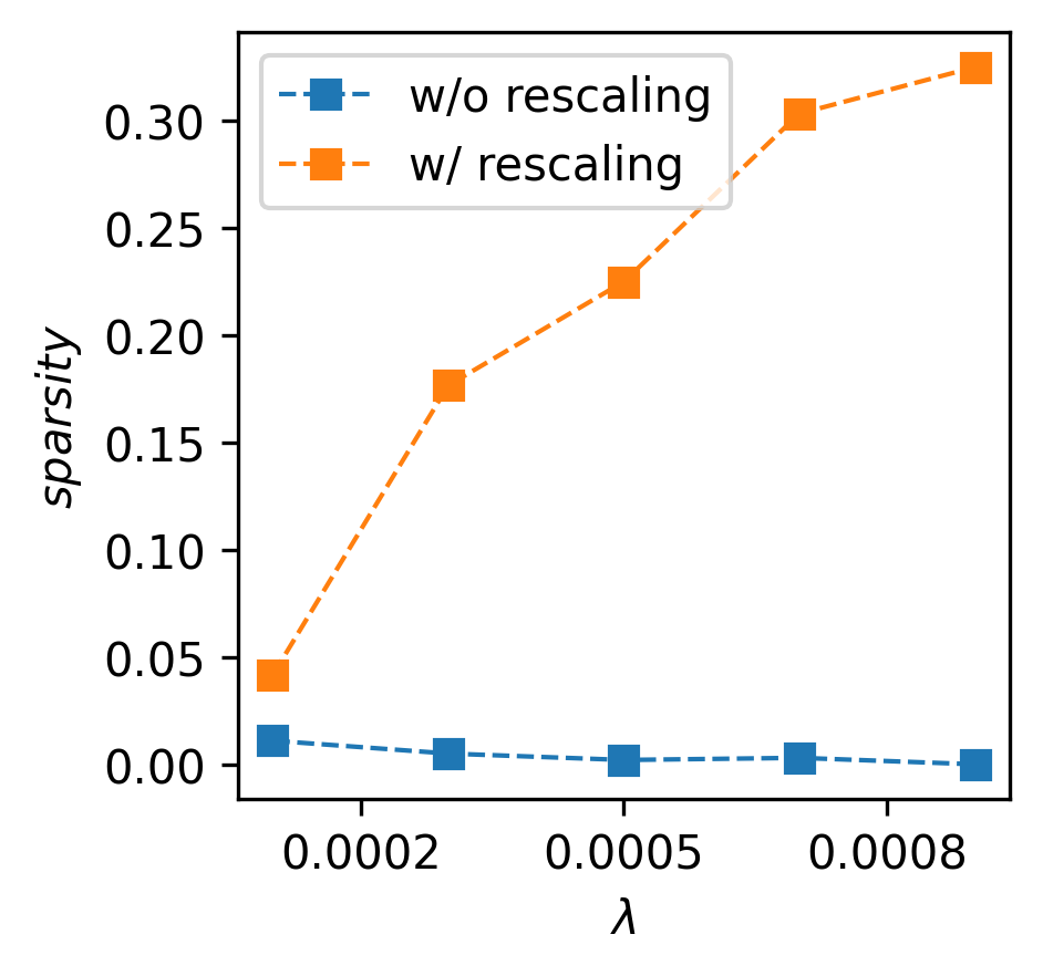
Two novel applications of this analysis are to learning a sparse model and a low-rank model. See Figure 3. We first apply it to a linear regression with rescaling symmetry. It is known that when both weight decay and rescaling symmetries are present, the solutions are sparse and identical to lasso (Ziyin & Wang, 2023). Our result shows that even without weight decay, the solutions are sparse at a large learning rate. Then, we consider a matrix factorization problem. Classical results show that the solutions are low-rank when weight decay is present (Srebro et al., 2004). Our result shows that even if there is no weight decay, SGD at a large learning rate or gradient noise converges to these low-rank saddles. The fact that these constrained structures disappear completely when the symmetry is removed supports our claim that symmetry is the cause of them.
Another strong piece of evidence for the relevance of the theory to real neural networks is that after training, the Hessian of the loss function is observed to contain many small negative eigenvalues, which hints at the convergence to saddle points (Sagun et al., 2016, 2017; Ghorbani et al., 2019; Alain et al., 2019). A related phenomenon is that of pathological Fisher information. Our result implies that the Fisher information is singular close to any symmetry solutions. Note that for a symmetry solution and any . Therefore, the Fisher information has a zero eigenvalue along the directions orthogonal to any mirror symmetry, in agreement with previous findings (Wei et al., 2008; Cousseau et al., 2008; Fukumizu, 1996; Karakida et al., 2019a, b).
2.5 Equivalence of Mirror Symmetries
Parts 3 and 4 of Theorem 1 imply that constrained solutions are favored when weight decay is used. These results can be stated in an alternative way: that every mirror symmetry plus weight decay has an equivalent. To see this, let the loss function be -symmetric, and . Let be an arbitrary weight, which we decompose as , where we define . Let us define an equivalent loss function . By definition, we have successfully constructed the equivalent of the original loss.
| (6) |
where we introduced . Therefore, along the symmetry-breaking direction, the loss function has an equivalent form. One can also show that is well defined as an -constrained loss function. If is differentiable, is differentiable except at . Thus, it suffices to show that the right derivative of with respect to exists at . As we have discussed, at , the expansion of is second order in . This means that the leading order term of is first order in , and so the penalty is well-defined for this loss function. Meanwhile, if there is no symmetry, this reparametrization will not work because will have a divergent derivative.
2.6 An Algorithm for Differentiable Constraint
Sparsity and low-rankness are typical structured constraints that practitioners often want to incorporate into their models (Tibshirani, 1996; Meier et al., 2008; Jaderberg et al., 2014). However, the known methods of achieving these structured constraints tend to be tailored for specific problems and based on nondifferentiable operations. Our theory shows that incorporating symmetries is a general and scalable way to introduce such constraints into deep learning. Consider solving the following constrained problem: s.t. as many elements of are zero as possible. Here, is a projection matrix. Our theory implies an algorithm for enforcing such constraints in a differentiable way: introducing an artificial -symmetry to the loss function encourages the constraint , which can be achieved by running GD on the following loss function:
| (7) |
where have the same dimension as and , where denotes the Hadamard product. We call the algorithm DCS, standing for differentiable constraint by symmetry. This parameterization introduces the mirror symmetry to which is a stationary condition. By Theorem 1, a sufficiently large ensures that is an energetically favored solution. Also, note that this parametrization is a “faithful” parametrization in the sense that it is always true that . A special case of this algorithm is the spred algorithm (Ziyin & Wang, 2023), which focuses on the rescaling symmetry and has been found to be efficient in model compression problems. See Section B for an application of the algorithm to ResNet18.


3 Examples and Experiments
Now, let us consider four examples where symmetry plays an important role in deciding the learned solution. While all the theorems in this section can be proved as corollaries of Theorem 1, we give independent proofs of them to bring some concreteness to the general theorem. The technical details of the experiments are in Section B.
3.1 Rescaling Symmetry Causes Sparsity
The simplest type of symmetry in deep learning is the rescaling symmetry. Consider a loss function for which the following equality holds for any , arbitrary vectors and :
| (8) |
For the rescaling symmetry and for all the problems we discuss below, it is also possible for to contain other parameters that are irrelevant to the symmetry: . Since having such or not does not change our result, we omit writting .
The following theorem states that this symmetry leads to sparsity in the parameters.
Theorem 2.
Let have the rescaling symmetry in Eq. (8). Then, for any , (1) if and , then and ; (2) for any fixed , , there exists such that for all , .
To prove this using the main theorem is simple. When the rescaling symmetry exists between two scalars and , there are two planes of mirror symmetry: and . Here, symmetry implies that is a symmetry solution, and symmetry implies that is a symmetry solution. Applying Theorem 1 to these two mirrors implies that and is a symmetry solution and obeys Theorem 2. When and are vectors of arbitrary dimensions and have the rescaling symmetry, one can identity the implied mirror symmetry as , and so : the loss function is symmetric to a simultaneous flip of all the signs of and . Applying Theorem 1 to this mirror again finishes the proof.
This symmetry usually manifests itself when part of the parameters is linearly connected. Previous works have used this property to either understand the inductive bias of neural networks or design efficient training algorithms. When the model is a fully connected ReLU network, Neyshabur et al. (2014) showed that having is equivalent to constraints of weights. Ziyin & Wang (2023) designed an algorithm to compress neural networks by transforming a parameter vector to , where is the Hadamard product.
For numerical evidence, see Figure 3-left and 4. Here, we consider a linear regression task with noisy Gaussian data, where the loss function is , where is either directly trained or parametrized as the Hadamard product of two-parameter vectors to artificially introduce rescaling symmetry: . We see that without such symmetry, the model never converges to a sparse solution, whereas the symmetrized parametrization converges to symmetry solutions, in agreement with the theory.
3.2 Rotation Symmetry Causes Low-Rankness
A more involved but common type of symmetry is the rotation symmetry, which also appears in a few slightly different forms in deep learning. This type of symmetry appears in matrix factorization problems, where it is a main cause of the emergence of saddle points (Li et al., 2019). It also appears in Bayesian deep learning (Tipping & Bishop, 1999; Kingma & Welling, 2013; Lucas et al., 2019; Wang & Ziyin, 2022), self-supervised learning (Chen et al., 2020; Ziyin et al., 2023b), and transformers in the form of key-query matrices (Vaswani et al., 2017; Dong et al., 2021).
Now, we show that rotation symmetry in the landscape leads to low rankness. We use the word “rotation” in a broad sense, including all orthogonal transformations. There are two types of rotation symmetry common in deep learning. In the first kind, we have for any ,
| (9) |
for any orthogonal matrix such that and is a set of weights viewed as a matrix or vector whose left dimension matches the right dimension of .
Theorem 3.
Let satisfy the rotation symmetry in Eq. (9). Then, for any index , vector and , (1) if , then ; (2) for any fixed , there exists such that for all , .222The notation denotes the matrix obtained by setting the -th singular value of to be zero.
Part 1 of the statement deserves a closer look. implies that is low-rank and is a left eigenvector of . That the gradient vanishes in this direction means that once the weight matrix becomes low-rank, it will always be low-rank for the rest of the training. To prove it using Theorem 1, we note that for any projection matrix , the matrix is an orthogonal matrix because . Therefore, the rotation symmetry already implies that for any and , . To apply the theorem, we need to view as a vector, and the corresponding reflection matrix is , a block-wise repetition of the matrix , where each block corresponds to a column of . By construction, is also a projection matrix. Since this holds for an arbitrary , one can choose to match the desired plane in Theorem 3, which can be then proved by invoking Theorem 1.
A more common symmetry is a “double” rotation symmetry, where depends on two matrices and and satisfies , for any orthogonal matrix and any and . Namely, the loss function is invariant if we simultaneously rotate two different matrices with the same rotation. In this case, one can show something similar: and for some fixed direction is the favored solution.
See Figure 3-mid, which shows that low-rank solutions are preferred in matrix factorization when the gradient noise is large (namely, when the learning rate is large or the label noise is strong), whereas such a tendency disappears when one removes the rotation symmetry by introducing a residual connection. An additional experiment with weight decay is presented in the Appendix.333It is now worthwhile to clarify the difference between continuous and discrete symmetries because rescaling and rotation symmetries are continuous transformations, and it seems like continuous symmetries can also cause these constraints. This is not true – the constraints are only consequences of the existence of reflection surfaces. Having continuous symmetries is one convenient way to induce certain types of mirror symmetry, but not the only way. Because transformers have the double rotation symmetry in the self attention, we also perform an experiment with transformers in an in-context learning task in Section B.6.
3.3 Permutation Symmetry Causes Homogeneity
The most common type of symmetry in deep learning is permutation symmetry. It shows up in virtually all architectures in deep learning. A primary and well-studied example is that in a fully connected network, the training objective is invariant to any pairwise exchange of two neurons in the same hidden layer. We refer to this case as the “special permutation symmetry” because it is a special case of the permutation symmetry we study below. Many recent works are devoted to understanding the special permutation symmetry (Simsek et al., 2021; Entezari et al., 2021; Hou et al., 2019).
Here, we study a more general and abstract type of permutation symmetry. The loss function has a permutation symmetry between parameter subsets and if, for any and ,444A special case is a hidden layer of a network; let and be the input and output weights of neuron , and , be the input and output weights of neuron . We can thus let and .
| (10) |
When there are multiple pairs that satisfy this symmetry, one can combine this pairwise symmetry to generate arbitrary permutations. From this perspective, permutation symmetries appear far more common than they are recognized. Another example is that a convolutional neural network is invariant to a pairwise exchange of two filters, which is rarely studied. A scalar rescaling symmetry can also be regarded as a special case of permutation symmetry.
Here, we show that the permutation symmetry tends to make the neurons become identical copies of each other (namely, encouraging to be as close to as possible).
Theorem 4.
Let satisfy the permutation symmetry in Eq. (10). Then, for any , (1) if , then ; (2) for any , there exists such that for all , .
To prove it, one can identify the projection as
| (11) |
Let denote a vector combination of both sets of the parameters. The permutation symmetry thus implies the mirror symmetry: . The symmetry solution is , and applying the master theorem to this mirror allows us to obtain Theorem 4.
This theorem implies that a permutation symmetry can be seen as a generalized form of ensembling smaller submodels.555It is not true that the origin is always favored when a mirror symmetry exists. Consider this loss: . A permutation symmetry exists between and . The condition is satisfied for all solutions of the loss whenever . Meanwhile, no solution satisfies . Restricted to fully connected networks, this type of homogeneous ensembling can be called a “neuron collapse.” This identification of the stationary subspace agrees with the result in Simsek et al. (2021). Special cases of this result have been proved previously. For a fully connected network, Fukumizu & Amari (2000) showed that the solutions of subnetworks are also solutions of the larger network, and Chen et al. (2023) demonstrated that these subnetwork solutions of fully connected networks can be attractive when the learning rate is large. Our result is more general because it does not restrict to the special permutation symmetry induced by fully connected networks. A novel application is that the networks have block-wise neurons and activation patterns whenever weight decay is present.
We train a Resnet18 on the CIFAR-10 dataset, following the standard training procedures. We compute the correlation matrix of neuron firing of the penultimate layer of the model, which follows a fully connected layer. We compare the matrix for both training with and without weight decay and for both pre- and post-activations (see Appendix B). See Figure 3-right, which shows that homogeneous solutions are preferred when weight decay is used, in agreement with the prediction of Theorem 1.
3.4 Loss of Plasticity and Neural Collapses
Also, our theory implies that the commonly observed loss of plasticity problem in continual and reinforcement learning (Lyle et al., 2023; Abbas et al., 2023; Dohare et al., 2023) is attributable to symmetries in the model. For a given task, weight decay or a finite learning rate makes the model converge to symmetry solutions, which tend to be low-capacity constrained solutions. If we train on an additional task, the capacity of the model can only decrease because the symmetry solutions are also stationary conditions, which SGD cannot escape. Fortunately, our theory suggests at least two ways to fix this problem: (1) use an alternative parameterization that explicitly removes the symmetry and/or (2) inject additive noise to the gradient to eliminate the stationary conditions. In fact, gradient noise injection is a known method to alleviate plasticity loss (Dohare et al., 2023). There are alternative ways to achieve (1). An easy way is to bias every (symmetry-relevant) parameter by a random bias: , where is a small fixed random variable.

A related phenomenon that symmetry can explain is the collapse of neural networks. The most common type of collapse is when the learned representation of a neural network spans a low-rank subspace of the entire available space, often leading to reduced expressive power. In Bayesian deep learning, a posterior collapse happens when the stochastic latent variables are low-rank (Lucas et al., 2019; Wang & Ziyin, 2022). This can be attributed to the double rotation symmetry of the encoder’s last layer weight and the decoder’s first layer weight. In self-supervised learning, a dimensional collapse happens when the representation of the last layer is low-rank (Tian, 2022), which has been found to be explained by the rotation symmetry of the last layer weight matrix. This also explains why many self-supervised learning methods focus on removing the symmetry (Bardes et al., 2021). The rank collapse that happens in self-attention may also be relevant (Dong et al., 2021). In supervised learning, the “neural collapse” happens when the learned representation of the penultimate learning becomes low-rank, which happens when weight decay is present (Papyan et al., 2020). Figure 3 shows that such a phenomenon can be attributed to the permutation symmetry in the fully connected layer. In summary, our result provides a unified perspective of the collapse phenomenon: collapses are caused by symmetries in the loss function. Our theory also suggests that these collapse phenomena have a natural interpretation as “phase transitions” in theoretical physics, where a collapse solution corresponds to a symmetric state with the “order parameter” being .666For example, see Ziyin et al. (2022) and Ziyin & Ueda (2022) for a study of these phase transitions in deep linear networks.
4 Related Works
A few related works study symmetries in specific deep-learning scenarios. To name a few primary examples, Fukumizu & Amari (2000) studies the permutation symmetry without weight decay or SGD training. Chen et al. (2023) studies permutation symmetry in fully connected networks with a large learning rate under SGD. However, it does not consider the role of weight decay nor its implication beyond fully connected nets. Ziyin & Wang (2023) studies rescaling symmetry when weight decay is present but does not study its Hessian or its connection to SGD training. Srebro et al. (2004) and the related works thereof study the matrix factorization with weight decay but not how SGD influences its solution nor how it relates to symmetry. In contrast, our result is useful for understanding both SGD and weight decay when symmetries are present. Lastly, Ziyin et al. (2024) studies the regularization effect of continuous symmetries under SGD, different from our focus on discrete symmetry. Besides, an interesting future problem is to leverage parameter-symmetries to learn data-space symmetries (Cohen & Welling, 2016; Bökman & Kahl, 2023) because learning group-invariant functions naturally involves special structures and constraints in the architecture.
5 Conclusion
In this work, we have presented a unified theory to understand the role of discrete symmetries in deep learning and studied their implications on gradient-based learning. We have shown that every mirror symmetry leads to a structured constraint of learning. This statement is examined from two different angles: (1) such solutions are favored when regularizations are applied; (2) they are favored when the gradient noise is strong (which can happen when the learning rate is large, the batch size is small, or the data is noisy). We substantiated our theoretical discovery with numerical examples of achieving common structures such as sparsity and low-rankness. We also discussed a variety of specific problems and phenomena and their relationship to symmetry. Our result is universal in that it only relies on the existence of the specified symmetries and does not rely on the properties of the loss function, model architectures, or data distributions. Per se, symmetry and its associated constraint are both good and bad. On the bad side, it limits the expressivity of the network and its approximation power. On the good side, it leads to more condensed models and representations, tends to ignore features that are noisy and can improve generalization capability thereby.
Acknowledgement
This research was conducted under the funding of the JSPS fellowship. The author is grateful for the constructive discussions with Prof. Masahito Ueda, Prof. Isaac Chuang, Hongchao Li, and Botao Li.
Impact Statement
This paper presents work whose goal is the theoretical aspects of artificial intelligence and, specifically, the symmetry of neural networks. The main implication is for the foundation algorithm design, and there seems to be no foreseeable negative societal consequence.
References
- Abbas et al. (2023) Abbas, Z., Zhao, R., Modayil, J., White, A., and Machado, M. C. Loss of plasticity in continual deep reinforcement learning. arXiv preprint arXiv:2303.07507, 2023.
- Alain et al. (2019) Alain, G., Roux, N. L., and Manzagol, P.-A. Negative eigenvalues of the hessian in deep neural networks. arXiv preprint arXiv:1902.02366, 2019.
- Anderson (1972) Anderson, P. W. More is different: Broken symmetry and the nature of the hierarchical structure of science. Science, 177(4047):393–396, 1972.
- Bardes et al. (2021) Bardes, A., Ponce, J., and LeCun, Y. Vicreg: Variance-invariance-covariance regularization for self-supervised learning. arXiv preprint arXiv:2105.04906, 2021.
- Bishop & Nasrabadi (2006) Bishop, C. M. and Nasrabadi, N. M. Pattern recognition and machine learning, volume 4. Springer, 2006.
- Bökman & Kahl (2023) Bökman, G. and Kahl, F. Investigating how relu-networks encode symmetries, 2023.
- Chen et al. (2023) Chen, F., Kunin, D., Yamamura, A., and Ganguli, S. Stochastic collapse: How gradient noise attracts sgd dynamics towards simpler subnetworks. arXiv preprint arXiv:2306.04251, 2023.
- Chen et al. (2020) Chen, T., Kornblith, S., Norouzi, M., and Hinton, G. A simple framework for contrastive learning of visual representations. In International conference on machine learning, pp. 1597–1607. PMLR, 2020.
- Cohen & Welling (2016) Cohen, T. and Welling, M. Group equivariant convolutional networks. In International conference on machine learning, pp. 2990–2999. PMLR, 2016.
- Cousseau et al. (2008) Cousseau, F., Ozeki, T., and Amari, S.-i. Dynamics of learning in multilayer perceptrons near singularities. IEEE Transactions on Neural Networks, 19(8):1313–1328, 2008.
- Dickman & Vidigal (2002) Dickman, R. and Vidigal, R. Quasi-stationary distributions for stochastic processes with an absorbing state. Journal of Physics A: Mathematical and General, 35(5):1147, 2002.
- Dinh et al. (2017) Dinh, L., Pascanu, R., Bengio, S., and Bengio, Y. Sharp Minima Can Generalize For Deep Nets. ArXiv e-prints, March 2017.
- Dohare et al. (2023) Dohare, S., Hernandez-Garcia, J. F., Rahman, P., Sutton, R. S., and Mahmood, A. R. Maintaining plasticity in deep continual learning. arXiv preprint arXiv:2306.13812, 2023.
- Dong et al. (2021) Dong, Y., Cordonnier, J.-B., and Loukas, A. Attention is not all you need: Pure attention loses rank doubly exponentially with depth. In International Conference on Machine Learning, pp. 2793–2803. PMLR, 2021.
- Entezari et al. (2021) Entezari, R., Sedghi, H., Saukh, O., and Neyshabur, B. The role of permutation invariance in linear mode connectivity of neural networks. arXiv preprint arXiv:2110.06296, 2021.
- Fukumizu (1996) Fukumizu, K. A regularity condition of the information matrix of a multilayer perceptron network. Neural networks, 9(5):871–879, 1996.
- Fukumizu & Amari (2000) Fukumizu, K. and Amari, S.-i. Local minima and plateaus in hierarchical structures of multilayer perceptrons. Neural networks, 13(3):317–327, 2000.
- Furstenberg & Kesten (1960) Furstenberg, H. and Kesten, H. Products of random matrices. The Annals of Mathematical Statistics, 31(2):457–469, 1960.
- Ghorbani et al. (2019) Ghorbani, B., Krishnan, S., and Xiao, Y. An investigation into neural net optimization via hessian eigenvalue density. In International Conference on Machine Learning, pp. 2232–2241. PMLR, 2019.
- Hastie et al. (2009) Hastie, T., Tibshirani, R., Friedman, J. H., and Friedman, J. H. The elements of statistical learning: data mining, inference, and prediction, volume 2. Springer, 2009.
- Hinrichsen (2000) Hinrichsen, H. Non-equilibrium critical phenomena and phase transitions into absorbing states. Advances in physics, 49(7):815–958, 2000.
- Hou et al. (2019) Hou, T., Wong, K. M., and Huang, H. Minimal model of permutation symmetry in unsupervised learning. Journal of Physics A: Mathematical and Theoretical, 52(41):414001, 2019.
- Ioffe & Szegedy (2015) Ioffe, S. and Szegedy, C. Batch normalization: Accelerating deep network training by reducing internal covariate shift. arXiv preprint arXiv:1502.03167, 2015.
- Jaderberg et al. (2014) Jaderberg, M., Vedaldi, A., and Zisserman, A. Speeding up convolutional neural networks with low rank expansions. arXiv preprint arXiv:1405.3866, 2014.
- Karakida et al. (2019a) Karakida, R., Akaho, S., and Amari, S.-i. Pathological spectra of the fisher information metric and its variants in deep neural networks. arXiv preprint arXiv:1910.05992, 2019a.
- Karakida et al. (2019b) Karakida, R., Akaho, S., and Amari, S.-i. Universal statistics of fisher information in deep neural networks: Mean field approach. In The 22nd International Conference on Artificial Intelligence and Statistics, pp. 1032–1041. PMLR, 2019b.
- Kingma & Welling (2013) Kingma, D. P. and Welling, M. Auto-encoding variational bayes. arXiv preprint arXiv:1312.6114, 2013.
- Li et al. (2019) Li, X., Lu, J., Arora, R., Haupt, J., Liu, H., Wang, Z., and Zhao, T. Symmetry, saddle points, and global optimization landscape of nonconvex matrix factorization. IEEE Transactions on Information Theory, 65(6):3489–3514, 2019.
- Lucas et al. (2019) Lucas, J., Tucker, G., Grosse, R., and Norouzi, M. Don’t blame the elbo! a linear vae perspective on posterior collapse, 2019.
- Lyle et al. (2023) Lyle, C., Zheng, Z., Nikishin, E., Pires, B. A., Pascanu, R., and Dabney, W. Understanding plasticity in neural networks. arXiv preprint arXiv:2303.01486, 2023.
- Meier et al. (2008) Meier, L., Van De Geer, S., and Bühlmann, P. The group lasso for logistic regression. Journal of the Royal Statistical Society: Series B (Statistical Methodology), 70(1):53–71, 2008.
- Neyshabur et al. (2014) Neyshabur, B., Tomioka, R., and Srebro, N. In search of the real inductive bias: On the role of implicit regularization in deep learning. arXiv preprint arXiv:1412.6614, 2014.
- Norris (1998) Norris, J. R. Markov chains. Number 2. Cambridge university press, 1998.
- Papyan (2018) Papyan, V. The full spectrum of deepnet hessians at scale: Dynamics with sgd training and sample size. arXiv preprint arXiv:1811.07062, 2018.
- Papyan et al. (2020) Papyan, V., Han, X., and Donoho, D. L. Prevalence of neural collapse during the terminal phase of deep learning training. Proceedings of the National Academy of Sciences, 117(40):24652–24663, 2020.
- Sagun et al. (2016) Sagun, L., Bottou, L., and LeCun, Y. Eigenvalues of the hessian in deep learning: Singularity and beyond. arXiv preprint arXiv:1611.07476, 2016.
- Sagun et al. (2017) Sagun, L., Evci, U., Guney, V. U., Dauphin, Y., and Bottou, L. Empirical analysis of the hessian of over-parametrized neural networks. arXiv preprint arXiv:1706.04454, 2017.
- Saxe et al. (2013) Saxe, A. M., McClelland, J. L., and Ganguli, S. Exact solutions to the nonlinear dynamics of learning in deep linear neural networks. arXiv preprint arXiv:1312.6120, 2013.
- Simsek et al. (2021) Simsek, B., Ged, F., Jacot, A., Spadaro, F., Hongler, C., Gerstner, W., and Brea, J. Geometry of the loss landscape in overparameterized neural networks: Symmetries and invariances. In International Conference on Machine Learning, pp. 9722–9732. PMLR, 2021.
- Srebro et al. (2004) Srebro, N., Rennie, J., and Jaakkola, T. Maximum-margin matrix factorization. Advances in neural information processing systems, 17, 2004.
- Tian (2022) Tian, Y. Deep contrastive learning is provably (almost) principal component analysis. arXiv preprint arXiv:2201.12680, 2022.
- Tibshirani (1996) Tibshirani, R. Regression shrinkage and selection via the lasso. Journal of the Royal Statistical Society: Series B (Methodological), 58(1):267–288, 1996.
- Tibshirani (2021) Tibshirani, R. J. Equivalences between sparse models and neural networks. Working Notes. URL https://www. stat. cmu. edu/~ ryantibs/papers/sparsitynn. pdf, 2021.
- Tipping & Bishop (1999) Tipping, M. E. and Bishop, C. M. Probabilistic principal component analysis. Journal of the Royal Statistical Society: Series B (Statistical Methodology), 61(3):611–622, 1999.
- Vaswani et al. (2017) Vaswani, A., Shazeer, N., Parmar, N., Uszkoreit, J., Jones, L., Gomez, A. N., Kaiser, Ł., and Polosukhin, I. Attention is all you need. Advances in neural information processing systems, 30, 2017.
- Wang & Ziyin (2022) Wang, Z. and Ziyin, L. Posterior collapse of a linear latent variable model. Advances in Neural Information Processing Systems, 35:37537–37548, 2022.
- Wei et al. (2008) Wei, H., Zhang, J., Cousseau, F., Ozeki, T., and Amari, S.-i. Dynamics of learning near singularities in layered networks. Neural computation, 20(3):813–843, 2008.
- Wu et al. (2018) Wu, L., Ma, C., et al. How sgd selects the global minima in over-parameterized learning: A dynamical stability perspective. Advances in Neural Information Processing Systems, 31, 2018.
- Wu et al. (2020) Wu, Y., Zhu, X., Wu, C., Wang, A., and Ge, R. Dissecting hessian: Understanding common structure of hessian in neural networks. arXiv preprint arXiv:2010.04261, 2020.
- Ziyin & Ueda (2022) Ziyin, L. and Ueda, M. Exact phase transitions in deep learning. arXiv preprint arXiv:2205.12510, 2022.
- Ziyin & Wang (2023) Ziyin, L. and Wang, Z. spred: Solving L1 Penalty with SGD. In International Conference on Machine Learning, 2023.
- Ziyin et al. (2021) Ziyin, L., Li, B., Simon, J. B., and Ueda, M. Sgd can converge to local maxima. In International Conference on Learning Representations, 2021.
- Ziyin et al. (2022) Ziyin, L., Li, B., and Meng, X. Exact solutions of a deep linear network. In Advances in Neural Information Processing Systems, 2022.
- Ziyin et al. (2023a) Ziyin, L., Li, B., Galanti, T., and Ueda, M. The probabilistic stability of stochastic gradient descent, 2023a.
- Ziyin et al. (2023b) Ziyin, L., Lubana, E. S., Ueda, M., and Tanaka, H. What shapes the loss landscape of self supervised learning? In The Eleventh International Conference on Learning Representations, 2023b. URL https://openreview.net/forum?id=3zSn48RUO8M.
- Ziyin et al. (2024) Ziyin, L., Wang, M., and Wu, L. The implicit bias of gradient noise: A symmetry perspective, 2024.
Appendix A Additional Related Works
Appendix B Experimental Concerns
B.1 Illustration of Stationary Conditions
See Figure 5.


B.2 Experimental Details and Additional Results for Figure 3
Here, we give the experimental details for the experiments in Figure 3.
For the sparsity experiments, we generate online data of batch size in the following way. The input is sampled from a diagonal normal distribution. The label , where is a noise term also sampled from a Gaussian distribution. The training proceeds with SGD without weight decay or momentum for iterations. The vanilla linear regression (labeled as “w/o rescaling”) is parameterized in the standard way: . The regressor with rescaling symmetry is parameterized as a Hadamard product, as in the spred algorithm (Ziyin & Wang, 2023): , where denotes the element-wise product.
For the low-rank experiment with matrix factorization, we also generate online data of batch size similarly. The input is sampled from a diagonal normal distribution. The label is , where controls the degree of noise in the label and can be seen as the effective signal-to-noise ratio in the data. Here, the noise vector have different variances: . The vanilla matrix factorization model is , where both and . The training proceeds with standard SGD without momentum or weight decay. For the inset figure, we parameterize the network through residual connections: , thus removing the rotation symmetry.
For the ResNet experiment, we train a standard ResNet18 with roughly 10M parameters in total on the CIFAR-10 dataset. The SGD algorithm uses a batch size of for epochs with a fixed learning rate of and momentum of , with varying degrees of weight decay. To plot the activation correlation, we take the penultimate layer neurons of the fully connected layer with dimension and compute the correlation matrix over their activation of unseen test points. The neurons are sorted according to the eigenvector with the largest eigenvalue of the correlation matrix to reveal its block structure. Importantly, the pre- and post-activations have a similar correlation structure, showing that the effect is not due to linearity but the permutation symmetry. See Figure 6 for the comparison between the pre- and post-activation correlations.
B.3 Experimental Detail for Continual Learning
Here, we give the experimental detail for the continual learning experiment in Figure 4.
For all the experiments in the figure, the training proceeds with Adam without momentum with a batch size of for steps. Every task consists of a dataset of data points drawn from the following distribution. The input is sampled from a diagonal normal distribution. The label , where is a noise term also sampled from a Gaussian distribution. The weights obtained from training on task is used as the initialization for task , which consists of another data points sampled in the same way. We train for tasks and record the number of dead neurons in the model. The dead neurons are defined as the number of parameters that have a vanishing gradient.
To have strong control over the experimental conditions, we use vanilla linear regression as a base model, which is shown in the solid curve. Because there is no symmetry in the model, the vanilla linear regression has a minimal level of dead neurons, and its number does not increase as the number of tasks increases.
In contrast, for a linear regression with augmented rescaling symmetry where we reparameterize every weight of the linear regressor by the Hadamard product of two independent weights (also see the previous section), the loss of plasticity problem emerges, and the number of dead neurons increases steadily as one train on more and more tasks. To show that symmetry is indeed the cause of the problem, we fix the loss of plasticity problem in this model with the two suggested methods. First, we inject a very weak Gaussian random noise with variance to the gradient every step. Because this removes the absorbing states, or equivalently the stationary conditions, the number of dead neurons reduces to the same level as vanilla regression. Alternatively, we bias every weight parameter by a random and fixed constant: , where is drawn from a Gaussian distribution with variance . Because this parametrization removes the symmetry in the model, it also fixes the loss of plasticity problem, as we expect from the theory.
B.4 Learning dynamics of the DCS Algorithm
To demonstrate the learning dynamics of the DCS algorithm, We consider training a sparse ResNet18 on CIFAR-10. Here, the training proceeds with SGD with momentum and batch size , consistent with standard practice. We use a cosine learning rate scheduler for 200 epochs. We compare the learning dynamics of vanilla ResNet18 and a ResNet18 with the rescaling symmetry on every parameter, where we reparametrize the original parameter vector as the Hadamard product of two vectors . Both models use a weight decay of 5e-4. We note that this special case of the DCS algorithm is identical to the spred algorithm (Ziyin & Wang, 2023). After training, both the vanilla model and the DCS model reach roughly test accuracy (with the DCS model higher by a small margin).
See Figure 7. As is clear, the training time required for a DCS model is similar to that of a vanilla model. In terms of memory cost, we note that DCS costs twice as much memory as the vanilla at batch size . However, at the batch size , the memory cost difference between the two is smaller than 10 percent.


B.5 Matrix Factorization
For completeness, we also include an experiment with regularized matrix factorization with GD. Here, we have a training set with datapoints, where each input data is i.i.d. from . The model has dimensions . We train with gradient descent for varying values of weight decay. See Figure 8.

B.6 Transformer
We perform an experiment with the simplest versions of transformer, with one or two single-head self-attention layers and without any MLP. Here, the input dimension is such that for each data point , elements of are i.i.d. from , and the target
| (12) |
where is a ground truth vector, generated also from . The tasks are the simplest type of in-context learning, where the first vectors serve as demonstrations of feature-target pairs, and the last row of is the feature that the model needs to predict, whose label is . Following this procedure, we construct a training set of data points, and the training proceeds with a full-batch Adam with a learning rate of and various weight decay values.
According to our theory, there is a double rotation symmetry between the key and query weights and . Therefore, we expect that as weight decay increases, the rank of the learned and drops. More importantly, as we discussed in the main text, they should drop together with each other. See Figure 10 and 10 for the result.
Appendix C Theoretical Concerns
C.1 A Formal Derivation of Eq. (5)
By Definition 2, the loss function has the -symmetry if for any
| (13) |
As we discussed, this means that for every data point , the per-sample Hessian takes the same block-wise structure outlined in Fig. 2. For this chapter, the most important consequence of Theorem 1 is that is a symmetry solution of for all .
We are interested in the atractivity of these solutions. The expansion of the per-sample loss to the second order gives:
| (14) |
where is a projection matrix, and is the component of that is orthogonal to the symmetry breaking subspace. Here, we care about when is attracted towards . The dynamics of is thus a stochastic linear dynamics:
| (15) |
where .
To proceed, we make the following assumption.
Assumption 2.
(Stationary background dynamics) The motion of is sufficiently slow that is a constant function in .
This also implies that any eigenvalue of also only depends on . This assumption holds when the time scale of relaxation for is far slower than that of or when the dynamics is already stationary, namely, close to convergence.
When Assumption 2 holds, and is rank-, this dynamics is analytically solvable. By Theorem 1, if is rank-, is an eigenvector of for all . Thus, the dynamics simplifies to a one-dimensional dynamics, where is the corresponding eigenvalue of :
| (16) |
C.2 Proofs
C.2.1 Proof of Theorem 1
Proof.
Part 1. Let . By assumption, we have . Now, consider a linearly transformed version of :
| (19) |
where is any unit vector in the image of . Note that we have the following relation:
| (20) |
Therefore, by definition of the mirror symmetry, we have that for all :
| (21) |
Dividing both sides by and taking the limit , we obtain
| (22) |
Because is arbitrary, one can select a set of such that they span the rows of , and we obtain that . This finishes part 1.
Part 2. Let . By symmetry, we have that for any and :888We use to denote the set of all vectors that is perpendicular to all the vectors in .
| (23) |
Let be an arbitrary vector in . Then, we also have that for any
| (24) |
Taking derivative over for both sides and let , we obtain
| (25) |
Taking derivative over and let , we obtain
| (26) |
Since is an arbitrary vector in and is an arbitrary in , this implies that
| (27) |
| (28) |
Namely, a subset of the eigenvectors of spans and the rest spans . This proves part 2.
To prove part 3, we first recognize that if we only look at the regularization part of the loss function, an orthogonal solution is always favored over a non-orthogonal solution. Let be an arbitrary solution such that . We decompose into an orthogonal part and a non-orthogonal part:
| (29) |
where and . Since and are orthogonal, we have that
| (30) |
Therefore, if
| (31) |
we have that
| (32) | ||||
| (33) | ||||
| (34) |
However, since we have , this proves part 3.
Part 4. By assumption, the smallest Hessian eigenvalue of is lower bounded by . Therefore, if , has a positive definite Hessian everywhere, implying that its gradients are monotone and that the global minimum is unique. Now, suppose there exists such that , , , and
| (35) |
Then,
| (36) |
This implies that the gradient is not monotone, which contradicts the assumption. Therefore, we have proved part 4. ∎
C.2.2 Proof of Theorem 2
Proof.
We first show part 1. The rescaling symmetry states that for any and ,
| (37) |
For an infinitesimal , this condition leads to
| (38) |
Taking the derivative of both sides over , we obtain
| (39) |
Therefore, the gradient of is . When both and are zero, . Likewise, we can show that . This proves part 1.
For part 2, let us denote the quantity as . Now, note that , and so setting
| (40) |
fulfills the requirement. Note that because is differentiable, the fraction always exists. This proves part 2.
∎
C.2.3 Proof of Theorem 3
Proof.
We focus on proving part 1. For an arbitrary and fixed index, , of the singular values of , we consider a continuous transformation of . Define a diagonal matrix for all , and define
| (41) |
We also define a transformed version of , which depends on an arbitrary vector :
| (42) |
With and , we define
| (43) |
We note two different features of this transformation: (1) is low-rank, and (2) for any , . To see this, note that there exists an orthogonal matrix such that
| (44) |
By the assumed symmetry of the loss function, we have . Because
| (45) |
we can take the derivative of of both sides of the equality to obtain a low-rank condition on the gradient width as a matrix:
| (46) |
In the limit , and so the equality leads to
| (47) |
Because this equality must hold for any , we have that must be a left eigenvector of with zero eigenvalues. Substituting into the gradient descent algorithm, we have
| (48) |
This proves part 1.
For part 2, we note that the Frobenious norm of a matrix is the sum of its squared singular values. Therefore, if we hold other singular values unchanged and shrink one of the singular values to , the regularization part of the loss function will strictly decrease. The rest of part 2 is the same as the proof of Theorem 2. ∎
C.2.4 Proof of Theorem 4
Proof.
The symmetry condition is
| (49) |
Taking the gradient of both sides with respect to , we obtain
| (50) |
When , we can write the above condition as
| (51) |
This proves the first part of the theorem.
We now prove the second part of the theorem. Let us define interpolation functions and :
| (52) |
| (53) |
With these definitions, we have . Also, we note that
| (54) |
which is the solution we want to compare with.
The loss function is given by
| (55) |
In contrast, for the homogeneous solution, the loss value is
| (56) |
The norms of the two solutions, and , can be compared:
| (57) |
where the inequality follows from the Cauchy-Schwarz inequality and the assumption that . Therefore, for any
| (58) |
. This proves the second part of the statement. ∎