Switchback effect of holographic complexity in multiple-horizon black holes

In recent years, quantum information perspectives have provided many useful techniques for studying the AdS/CFT correspondence. This idea has aroused more and more attention to the concept of “quantum circuit complexity”, which is defined as the number of the elementary gates in the optimal circuit from a given state to a target state Watrous ; Aaronson ; Susskind01 ; Susskind02 ; Susskind03 . From the perspective of holography, two complementary conjectures for the bulk description of the complexity of boundary states have been proposed: the “complexity equals volume” (CV) Susskind03 ; D.Stanford and the “complexity equals action” (CA) BrL ; BrD conjectures. The CV conjecture states that the circuit complexity of a quantum state $|\psi(t_{L},t_{R})\rangle$ in boundary strongly-coupled system is dual to the volume $V$ of the Einstein-Rosen bridge anchored at the time slices $t_{L}$ and $t_{R}$ on the boundary, i.e.,

$\displaystyle\begin{aligned} C_{V}\left(|\psi(t_{L},t_{R})\rangle\right)=\frac{V}{G\ell_{\text{AdS}}}\,.\end{aligned}$

(1)

On the other hand, the CA conjecture states that the complexity of boundary state is given by evaluating the full on-shell action of the bulk gravitational theory on the Wheeler-DeWitt (WDW) patch, which is the causal development of a spacelike bulk surface (Cauchy surface) connected the boundary timeslices $t_{L}$ and $t_{R}$, i.e.,

$\displaystyle C_{A}\left(|\psi(t_{L},t_{R})\rangle\right)\equiv\frac{I_{\text{WDW}}}{\pi\hbar}\,.$

(2)

These conjectures have attracted researchers to study the complexity of the strongly-coupled quantum system from the perspective of the holographic principle Susskind1 ; Susskind2 ; Susskind3 ; Susskind4 ; Susskind5 ; Susskind6 ; Zhao1 ; Zhao2 ; Zhao3 ; Myers1 ; Myers2 ; Myers3 ; Myers4 ; Myers5 ; Myers6 ; Myers7 ; Chapman1 ; Chapman2 ; Fan1 ; Fan2 ; Fan3 ; Fan4 ; Jiang1 ; Jiang2 ; Jiang3 ; Jiang4 ; Jiang5 ; Jiang6 ; Jiang7 ; Jiang8 ; An1 ; An2 ; An3 ; Yang1 ; Yang2 ; Yang3 ; Yang4 ; Yang5 ; Yang6 ; 1 ; 2 ; 3 ; 4 ; 5 ; 6 ; 7 ; 8 ; 9 ; 10 ; 11 ; 12 ; 13 ; 14 ; 15 ; 16 ; 17 ; Moosa ; Nally:2019rnw ; Auzzi:2019mah ; Tanhayi:2018gcj ; s1 ; s2 ; s3 ; s4 .

The concepts of the local and global quantum quenches have been widely used to study the holographic complexity. The local quench is the process when the system evolves after a local perturbation. It was argued that the holographic dual of this process is given by the black hole geometry perturbed by the particle falling on the horizon local1 ; local2 ; local3 ; local4 ; local5 . Based on this setup, Lloyd’s bound Lloyd of the complexity in the boundary system has been tested under the local quench by using the holographic conjecturesLQ1 ; LQ2 ; LQ3 . If the perturbation is global, the process is called a global quench. The holographic dual of this process is given by the Vaidya geometry, which is equipped with a thin shell of null fluid collapse (shockwave) G1 ; G2 ; G3 ; G4 ; G5 ; G6 ; G7 ; G8 . Based on this duality, the time-dependence of the complexity in the boundary quantum field system has been studied by using different holographic complexities Chapman1 ; Chapman2 ; Moosa ; Fan2 ; Jiang2 ; Yang3 ; Auzzi:2019mah ; Tanhayi:2018gcj .

It has been generally argued in D.Stanford ; Susskind5 that the quantum complexity in chaos system should exhibit the switchback effect when this system is perturbed by a quantum quench, which can be described by a precursor $\mathcal{O}(t)=U^{\dagger}(t)\mathcal{O}U(t)$ of a simple perturbation operator $\mathcal{O}$. Since $\mathcal{O}$ is a very simple operator, at a very early time, it can be regarded as a unit operator and then the complexity does not grow. However, for a chaotic system, at a very large time compared to the scrambling time $t_{\text{scr}}^{\star}$, the operator $\mathcal{O}$ will disrupt the time-reversed evolution and the complexity will become twice the complexity of the evolution operator $U(t)$ D.Stanford . This property of the quantum complexity under the quantum quench is known as the switchback effect D.Stanford . This feature plays an important role to examine the definitions the complexity.

Although lots of researchers focused on the calculation of the circuit complexity in quantum field theory jiang1 ; jiang2 ; myers1 ; myers2 ; myers3 ; myers4 ; yang1 ; yang2 ; yang3 ; yang4 ; f1 ; f2 ; f3 ; f4 , there is still a lack of a valid method to evaluate the circuit complexity in the strongly-coupled system. Therefore, some researchers used the holographic complexity in the Vaidya black holes for Einstein gravity to study the switchback effect in the boundary strongly-coupled system Susskind5 ; D.Stanford ; Chapman2 ; Jiang2 . However, in the context of AdS/CFT, the Einstein gravity in bulk is dual to the strongly-coupled quantum field with infinite $N$ or infinite coupling effects. A natural question for us is to ask whether the switchback effect is a general feature of the strongly-coupled quantum system and independent on the explicit of the quantum state as well as the quantum theory. As we all know, the boundary quantum field theory with finite $N$ and finite coupling effects are corresponding to a gravitational theory with higher curvature corrections. Therefore, in this paper, we would like to use the CA conjecture to show whether the switchback effect also exists in the strongly-coupled quantum system with finite $N$ and finite coupling effect under a global quantum quench.

Recently, some authors found that once the higher curvature corrections are taken into account, the neutral (single-horizon) black holes will have a divergent complexity growth rate since the WDW patch will go arbitrarily near the singularity Nally:2019rnw ; Jiang8 . However, this does not happen for multiple-horizon black holes due to the different causal structure including at least two horizons. Moreover, most of the previous researches imply that the CA complexity for the neutral black hole can be obtained by taking the limit of its corresponding multiple-horizon counterpart Yang6 ; s1 ; s2 ; s3 ; s4 . Therefore, in order to reflect some universal features of the CA complexity and avoid the divergent result of the neutral case, in this paper, we would like to focus on the black holes which have at least two Killing horizons. Generally, these black holes capture some extra conserved charges, such as the angular momentum and electric charge. From the viewpoint of the holography, they are dual to the boundary quantum state which also contains some extra conserved charges. Therefore, our investigations can also reflect the influence of the extra conserved charges on the complexity in the boundary quantum system.

The above statements show that the main task of this paper is to evaluate the CA complexity in the Vaidya geometry equipped with a light shockwave. By analyzing this geometry in Sec.II, we can see that at the large time limit, the dynamical points will approach the Killing horizons. Then, the actions that we need to evaluate are in the regions which are connected to the Killing horizons and can be generated by the corresponding Killing vectors. This property allows us to express this action as some boundary integrals based on Iyer-Wald formalism IW . Therefore, in the following, we would like to utilize the Iyer-Wald formula to derive some general expressions of the CA complexity at large times.

The remainder of our paper is organized as follows: in Sec. II, we first study the geometry of the stationary black hole with a thin shell of null fluid collapse. In Sec. III, we briefly review the Iyer-Wald formalism for a invariant theory. In Sec. IV, we investigate the switchback effect of the CA complexity in a multiple-horizon black hole for a general higher curvature gravitational theory coupled with arbitrary matter fields. In Sec. V, we compare our holographic results with the circuit behaviors.

As mentioned above, the stationary multiple horizons of the black holes are caused by the extra conserved charges of the spacetime. In the context of AdS/CFT, these black holes are dual to the thermofield double (TFD) states

$\displaystyle\begin{aligned} |\text{TFD}\rangle=Z^{-1/2}\sum_{\alpha}e^{-\beta(E_{\alpha}+\mu Q_{\alpha})/2}|E_{\alpha},Q_{\alpha}\rangle_{\text{L}}|E_{\alpha},-Q_{\alpha}\rangle_{\text{R}}\end{aligned}$

on the boundary strongly-coupled quantum field theory TFD , where we have denoted the subscripts L and R to the left and right boundaries of the multiple-horizon black hole geometry individually. Here $E_{\alpha}$ and $Q_{\alpha}$ are corresponding to the eigenvalues of the energy and extra conserved charges separately. The time evolution of the TFD state is obtained by

$\displaystyle\begin{aligned} |\text{TFD}(t_{L},t_{R})\rangle=U_{L}(t_{L})U_{R}(t_{R})|\text{TFD}\rangle\,.\end{aligned}$

(4)

where

$\displaystyle\begin{aligned} U_{L}(t_{L})=e^{-i(H_{L}+\mu Q_{L})t_{L}}\,,U_{R}(t_{R})=e^{-i(H_{R}-\mu Q_{R})t_{R}}\end{aligned}$

(5)

are the time evolution operators corresponding to the left and right quantum system. We can see that this state is invariant under the shift transformation

$\displaystyle\begin{aligned} t_{L}\to t_{L}+\Delta t\,,\ \ \ \ \ t_{R}\to t_{R}-\Delta t\,.\end{aligned}$

(6)

In this paper, we would like to investigate the switchback effect of the complexity. Following the setup in Refs. D.Stanford ; Susskind5 ; Chapman2 , we consider the perturbation of the TFD state,

$\displaystyle\begin{aligned} |\text{TFD}\rangle_{\text{pert}}&=\mathcal{O}_{R}(-t_{w})|\text{TFD}\rangle\\ &=U_{R}(t_{w})\mathcal{O}_{R}U_{R}^{\dagger}(t_{w})|\text{TFD}\rangle\end{aligned}$

(7)

where the precusor $\mathcal{O}_{R}(-t_{w})=U_{R}(t_{w})\mathcal{O}_{R}U_{R}^{\dagger}(t_{w})$ is the perturbation operator inserted into the right sight quantum system at time $-t_{w}$, and $\mathcal{O}_{R}$ is a localized simple operator. In the chaos quantum system, $U_{R}(t_{w})$ and $U_{R}^{\dagger}(t_{w})$ will approximately cancel until times of the order of the scrambling time $t_{\text{scr}}^{\star}$ D.Stanford and the state would keep unchanged, i.e., the complexity growth rate is vanishing. For $t_{w}\gg t_{\text{scr}}^{\star}$, the complexity growth rate of $\mathcal{O}(t_{w})$ is just twice the rate of the evolution operator $U_{R}(t_{w})$. This nontrivial feature is connected to the switchback effect D.Stanford ; Susskind5 . Evolving the perturbed state in the right and left time gives

$\displaystyle\begin{aligned} |\text{TFD}(t_{L},t_{R})&\rangle_{\text{pert}}=U_{L}(t_{L})U_{R}(t_{R})|\text{TFD}\rangle_{\text{pert}}\\ &=U_{R}(t_{R}+t_{w})\mathcal{O}_{R}U_{R}(t_{L}-t_{w})|\text{TFD}\rangle\,.\end{aligned}$

(8)

In the holographic context, the dual geometry in the bulk to above perturbed system is AdS-Vaidya spacetime with multiple horizons source by a thin shell of null fluid collapses. It can be described by the metric ansatz

$\displaystyle ds^{2}=ds^{2}_{2}\mathcal{H}(v+t_{w})+ds^{2}_{1}\left[1+\mathcal{H}(v+t_{w})\right],$

(9)

where $\mathcal{H}(v)$ is the Heaviside step function, and

$\displaystyle\begin{aligned} &ds^{2}_{i}=\alpha_{i}(r,y)\left[-f_{i}(r)dv^{2}+2dvdr\right]\\ &+\gamma_{AB}^{(i)}(r,y)\left[dy^{A}-\Omega^{(A)}_{i}(r,y)dv+\frac{\Omega^{(A)}_{i}(r,y)}{f_{i}(r)}dr\right]\\ &\times\left[dy^{(B)}-\Omega^{(B)}_{i}(r,y)dv+\frac{\Omega^{(B)}_{i}(r,y)}{f_{i}(r)}dr\right]\,,\end{aligned}$

(10)

where $i=1,2$ describes a multiple-horizon stationary black hole, the indexes $A,B$ denote the coordinates of the codimension-two surface, $\Omega^{(A)}$ is some component of the metric which becomes the angular velocity of the black holes when it evaluates on the Killing horizon. The metric in (LABEL:ds2) is a generalization from most stationary axisymmetric black holes in general relativity or other theories of gravity, such as: Kerr-AdS(dS) black holes, Myers-Perry black holes Myers:1986un , rotating Bardeen black holes Bambi:2013ufa , rotating Hyward black holes Bambi:2013ufa , rotating charged cylindrical black holes Lemos:1995cm , Kerr-MOG black holes Moffat:2014aja , Kerr-Sen black holesSen:1992ua , Kerr-Newman-Taub-NUT-AdS black holes Taub1 , Gauss-Bonnet black holes GB , rotating black holes in a Randall-Sundrum brane RS , and charged accelerating AdS black holes caads .

By virtue of the second law of thermodynamics for black holes, we will set $r_{+,2}>r_{+,1}$ with horizon radius $r_{\pm,i}$ determined by $f_{i}(r_{\pm,i})=0$. This line element describes an infinitely thin shell collapse which generates a shape transition from a black hole with the metric $ds_{1}^{2}$ to another one with $ds^{2}_{2}$. For the convenience of later calculations, we would like to introduce the tortoise coordinates as

$\displaystyle\begin{aligned} v_{R}&<-t_{w}:\ \ \ \ \ r_{1}^{*}(r)=\int\frac{dr}{f_{1}(r)}\,,\\ v_{R}&>-t_{w}:\ \ \ \ \ r_{2}^{*}(r)=\int\frac{dr}{f_{2}(r)}\,.\end{aligned}$

(11)

When the position considered is near the horizon, i.e., $r\simeq r_{\pm,i}$, we have

$\displaystyle r_{i}^{*}(r)\simeq\frac{1}{2\kappa_{\pm,i}}\ln\left|\frac{r-r_{\pm,i}}{r+r_{\pm,i}}\right|\,,$

(12)

where

$\displaystyle\begin{aligned} \kappa_{\pm,i}=\frac{|f^{\prime}_{i}(r_{\pm})|}{2}\end{aligned}$

(13)

is the surface gravity corresponding to the Killing horizons. Using these coordinates, one can also define an “outgoing” null coordinate $u$ and auxiliary time coordinate $t$ as

$\displaystyle u_{i}\equiv v-2r^{*}_{i}(r),\ \ \ \ \ \ \ t_{i}\equiv v-r^{*}_{i}(r)\,.$

(14)

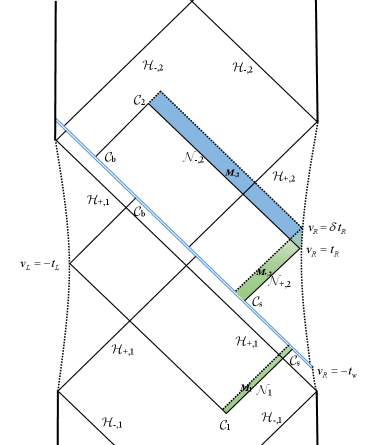
According to the CA conjecture (2), computing the quantum complexity of the boundary state is equivalent to evaluating the full action within the WDW patch. As is shown in Fig.1, the geometry of the WDW patch is characterized by some dynamical points: $r_{1}$ and $r_{2}$, the points where the past/future null boundaries of the WDW patch meet inside the horizon; $r_{s}$ and $r_{b}$, the positions where the right past and left future boundaries meet the shockwave. Moreover, in order to regulate the divergence caused by the asymptotic infinity, a cut-off surface $r=r_{\Lambda}$ is also introduced.

Performing the tortoise coordinates, one can find that these dynamical positions $r_{s},r_{b},r_{1}$ and $r_{2}$ yield

$\displaystyle\begin{aligned} t_{w}+2r_{2}^{*}(r_{s})&=-t_{R}\,,\\ t_{w}+2r_{1}^{*}(r_{b})&=t_{L}\,,\\ t_{w}+2r_{1}^{*}(r_{s})&=t_{L}+2r_{1}^{*}(r_{1})\,,\\ t_{w}+2r_{2}^{*}(r_{b})&=-t_{R}+2r_{2}^{*}(r_{2})\,.\\ \end{aligned}$

(15)

For the cases with light shockwave, there exists a scrambling time

$\displaystyle t_{\text{scr}}^{*}=\frac{1}{2\pi T_{+,1}}\ln\frac{2}{\delta}\,,$

(16)

which divides the evolution into two asymptotic regions. Here we have denoted

$\displaystyle\begin{aligned} T_{\pm,i}=\frac{1}{4\pi}f_{i}^{\prime}(r_{\pm,i})\,,\ \ \delta=\frac{r_{+,2}}{r_{+,1}}-1\,.\end{aligned}$

(17)

For the case with a light shockwave, the scrambling time becomes very large. According to the expressions (15), we can see that the dynamical point $r_{s}$ approaches the horizon $\mathcal{H}_{2,+}$. Then, when $t_{w}-t_{L}>t_{\text{scr}}^{*}$ and $t_{w}+t_{R}>t_{\text{scr}}^{*}$, we have

$\displaystyle\begin{aligned} 2r_{1}^{*}(r_{1})&=t_{w}-t_{L}-t_{\text{scr}}^{*}\,,\\ 2r_{2}^{*}(r_{2})&=t_{w}+t_{R}-t_{\text{scr}}^{*}\,.\end{aligned}$

(18)

These expressions imply that the scrambling time $t_{\text{scr}}^{*}$ is a transition position for $r_{i}$ between $r_{+,i}$ and $r_{-,i}$. Then, in the limit of large $t_{w}$, we have $r_{s}\to r_{+,2}$, $r_{b}\to r_{+,1}$ and $r_{i}\to r_{-,i}$.

Finally, we consider the behaviors of the null segment which crosses the shockwave. According to the line element (LABEL:ds2), it is easy to check that

$\displaystyle\begin{aligned} l_{a}=l^{a}_{2}\mathcal{H}(r-r_{s})+\Lambda_{s}l_{1}^{a}\left[1-\mathcal{H}(r-r_{s})\right]\,,\\ \tilde{l}_{a}=\tilde{l}^{a}_{1}\mathcal{H}(r-r_{b})+\Lambda_{b}\tilde{l}_{2}^{a}\left[1-\mathcal{H}(r-r_{b})\right]\,,\\ \end{aligned}$

(19)

with

$\displaystyle\begin{aligned} l_{i}^{a}=-(dv)_{a}+\frac{2}{f_{i}(r)}(dr)_{a}\,,\ \ \ \ \Lambda_{s}=\frac{f_{1}(r_{s})}{f_{2}(r_{s})}\,,\\ \tilde{l}_{i}^{a}=-(dv)_{a}+\frac{2}{f_{i}(r)}(dr)_{a}\,,\ \ \ \ \Lambda_{b}=\frac{f_{2}(r_{b})}{f_{1}(r_{b})}\,,\end{aligned}$

(20)

are the affine null generator of the past right and future left null boundaries, individually. We can find that $\mathcal{L}_{\zeta}l^{a}_{i}=0$ if $\zeta^{a}$ is a Killing vector field, such as the stationary Killing vector $t^{a}=(\partial/\partial v)^{a}$ or the axial Killing vector $\varphi^{a}_{(\mu)}$. Then, using Eq. (15), one can further obtain

$\displaystyle\begin{aligned} &\frac{d\ln\Lambda_{s}}{dt_{R}}\simeq-2\pi T_{+,2}\,,\ \ \ \ \frac{du_{2,s}}{dt_{R}}=\Lambda_{s}^{-1}\simeq 0\,,\\ &\frac{d\ln\Lambda_{b}}{dt_{L}}\simeq 2\pi T_{+,1}\,,\ \ \ \ \ \ \ \frac{du_{1,b}}{dt_{L}}=-\Lambda_{b}^{-1}\simeq 0\,,\end{aligned}$

(21)

at the large time limit. These results imply that the past right null segment before shockwave as well as the future right null segment after shockwave keep almost unchanged when we vary the left or right boundary times.

According to the discussion in the last section, we can see that all of the dynamical points of WDW patch are located on the horizons $\mathcal{H}_{\pm,i}$ in the limit of large time $t_{w}$. The integral region for calculating the change of the bulk action can be generated by the diffeomorphism related to the Killing vector field of the Killing horizon. Using the Stokes’ theorem, we can express these action as some boundary integrals related to the Killing vector fields. On the other hand, Iyer and Wald IW perform the differential form to obtain the relationship between the conserved charges related to some vector fields and the action integrals. Therefore, it might be possible for us to derive some general expressions of the CA complexity at the large time limit based on the Iyer-Wald formalism. Next, we would like to give a brief review of the Iyer-Wald formalism for a general diffeomorphism invariant theory, which is described by a Lagrangian $\bm{L}=\mathcal{L}\bm{\epsilon}$ where the dynamical fields consist of a Lorentz signature metric $g_{ab}$ and other fields $\psi$. Following the notation in IW , we use boldface letters to denote differential forms and collectively refer to $(g_{ab},\psi)$ as $\phi$. Generally, the action can be divided into the gravity part and matter part, i.e., $\bm{L}=\bm{L}_{\text{grav}}+\bm{L}_{\text{mt}}$. The variation of the gravitational part with respect to $g_{ab}$ is given by

$\displaystyle\delta\bm{L}_{\text{grav}}=\bm{E}_{g}^{ab}(\phi)\delta g_{ab}+d\bm{\Theta}(\phi,\delta g)\,,$

(22)

where $\bm{E}_{g}^{ab}(\phi)$ is locally constructed out of $\phi$ and its derivatives and $\bm{\Theta}$ is locally constructed out of $\phi,\,\delta g_{ab}$ and their derivatives. The equation of motion can be read off as

$\displaystyle\bm{E}_{g}^{ab}(\phi)=\frac{1}{2}T^{ab}\bm{\epsilon}\,,$

(23)

where

$\displaystyle T^{ab}=-\frac{2}{\sqrt{-g}}\frac{\delta\sqrt{-g}\mathcal{L}_{\text{mt}}}{\delta g_{ab}}=-g^{ab}\mathcal{L}_{\text{mt}}-2\frac{\delta\mathcal{L}_{\text{mt}}}{\delta g_{ab}}$

(24)

is the stress-energy tensor of the matter fields. Let $\zeta^{a}$ be the infinitesimal generator of a diffeomorphism. Exploiting the Bianchi identity $\nabla_{a}T^{ab}=0$, one can obtain the identically conserved current for a generic background metric $g_{ab}$ as

$\displaystyle\begin{aligned} \bm{J}[\zeta]&=\bm{\Theta}(\phi,\zeta)-\zeta\cdot\bm{L}_{\text{grav}}+s_{\zeta}\cdot\bm{\epsilon}\,,\end{aligned}$

(25)

where $s^{a}_{\zeta}\equiv T^{ab}\zeta_{b}$ and $\bm{\Theta}(\phi,\zeta)=\bm{\Theta}(\phi,\mathcal{L}_{\zeta}g_{ab})$. Since $\bm{J}$ is closed, there exists a Noether charge $(n-2)$-form $\bm{K}[\zeta]$ such that $\bm{J}[\zeta]=d\bm{K}[\zeta]$. With similar arguments in IW , this $(n-2)$-form can always be expressed as

$\displaystyle\bm{K}=\bm{W}_{c}\zeta^{c}+\bm{X}^{cd}\nabla_{[c}\zeta_{d]}\,,$

(26)

where

$\displaystyle\left(\bm{X}^{cd}\right)_{c_{3}\cdots c_{n}}=-E_{R}^{abcd}\bm{\epsilon}_{abc_{3}\cdots c_{n}}\,,$

(27)

is the Wald entropy density in which

$\displaystyle E_{R}^{abcd}=\frac{\delta\mathcal{L}_{\text{grav}}}{\delta R_{abcd}}\,.$

(28)

Particularly, when $\zeta^{a}$ is taken to a rotational Killing vector $\varphi^{a}$ in an axisymmetric spacetime, by using this $(n-2)$-form, we can construct a conserved charge

$\displaystyle J[\varphi]=-\int_{\mathcal{C}_{\infty}}\bm{K}[\varphi]\,,$

(29)

where $\mathcal{C}_{\infty}$ denotes a $(n-2)$-dimensional surface at the asymptotic infinity. It can be interpreted as the angular momentum of the black hole in an arbitrary asymptotic spaceWSS . For a general higher curvature gravitational theory, it is given by

$\displaystyle J[\varphi]=-\int_{\mathcal{C}_{\infty}}\left(\bm{X}^{cd}\nabla_{[c}\varphi_{d]}-2\varphi_{b}\nabla_{a}\bm{X}^{ab}\right)\,.$

(30)

Moreover, if we set $\zeta^{a}$ to a Killing vector, by substituting (24) into (25), one can obtain

$\displaystyle\zeta\cdot\bm{L}=d\left(\bm{\Lambda}[\zeta]-\bm{K}[\zeta]\right)\,,$

(31)

where $\bm{\Lambda}[\zeta]$ is a $(n-2)$-form and constructed by

$\displaystyle\chi_{\zeta}\cdot\bm{\epsilon}=d\bm{\Lambda}[\zeta]\,,\ \text{with}\ \ \chi^{a}_{\zeta}=-2\frac{\delta\mathcal{L}_{\text{mt}}}{\delta g_{ab}}\zeta_{b}\,.$

(32)

In this section, we start to evaluate the derivative of the complexity of formation with respect to $t_{w}$ (the slope of the complexity of formation). Here the complexity of formation is defined as the extra complexity required to prepare the two copies of the quantum field theory in the TFD state compared to simply preparing each of the copies in the vacuum state, i.e.,

$\displaystyle\Delta C=C\left(|\text{TFD}\rangle\right)-C\left(|0\rangle_{L}\otimes|0\rangle_{R}\right)$

(33)

In the context of AdS/CFT, it is dual to the difference between the holographic complexity for a black hole and that for two copies of the vacuum geometry at $t_{R}=t_{L}=0$. Therefore, in the following, it is sufficient to restrict our attention to the case $t_{L}=t_{R}=0$. By considering the shift symmetry to the antisymmetric time evolution of the complexity, i.e.,

$\displaystyle t_{R}\to t_{R}-\delta t\,,\ \ t_{L}\to t_{L}+\delta t\,,\ \ t_{w}\to t_{w}+\delta t\,,$

(34)

we can further obtain

$\displaystyle\frac{d\Delta C}{dt_{w}}=\left[\frac{dC_{A}}{dt_{R}}-\frac{dC_{A}}{dt_{L}}\right]_{t_{L}=t_{R}=0}\,,$

(35)

where we have used the fact that the complexity in vacuum geometry is time-independent. Then, using CA conjecture (2), obtaining the slope of the complexity of formation amounts to finding the change of the full action $I$ within the WDW patch, i.e.,

$\displaystyle\begin{aligned} \delta I_{L}&=I(t_{L}+\delta t_{L},t_{R})-I(t_{L},t_{R})\,,\\ \delta I_{R}&=I(t_{L},t_{R}+\delta t_{R})-I(t_{L},t_{R})\,.\end{aligned}$

(36)

For a general higher curvature gravity, the full action can be expressed as Jiang3

$\displaystyle\begin{aligned} I=&\int_{M}\bm{L}+\int_{\mathcal{C}}\bm{s}\eta+\int_{\mathcal{N}}d\lambda\bm{s}\kappa+\int_{\mathcal{N}}d\lambda\partial_{\lambda}\bm{s}\ln\left(l_{\text{ct}}\Theta\right),\end{aligned}$

(37)

where $\bm{s}=\bm{X}^{cd}\bm{\epsilon}_{cd}$ is the Wald entropy density, $\lambda$ is the parameter of the null generator $k^{a}$ on the null segment, $\kappa$ measures the failure of $\lambda$ to be an affine parameter which is derived from $k^{a}\nabla_{a}k^{b}=\kappa k^{b}$, $\Theta=\nabla_{a}k^{a}$ is the expansion scalar, and $l_{\text{ct}}$ is an arbitrary length scale.

As mentioned in the last section, there are two asymptotic regions: $t_{w}\ll t^{*}_{\text{scr}}$ and $t_{w}\gg t^{*}_{\text{scr}}$. In the first region with $t_{w}\ll t^{*}_{\text{scr}}$, we can simply approximate $ds_{1}^{2}\simeq ds_{2}^{2}$ at the limit of light shockwave, i.e., the complexity of formation is same as the unperturbed geometry. Then, by utilizing the shift symmetry, the slope of complexity of formation vanishes, i.e.,

$\displaystyle\left.\frac{d\Delta C}{dt_{w}}\right|_{t_{w}\ll t^{*}_{\text{scr}}}=0\,.$

(38)

Then, we consider the second region with $t_{w}\gg t^{*}_{\text{scr}}$. Under this limit, the joints $\mathcal{C}_{i}$ and $\mathcal{C}_{s}$ approach the inner horizon $\mathcal{H}_{-,i}$ and the outer horizon $\mathcal{H}_{+,2}$ respectively, and the left future and right past boundary of the WDW patch become the segment of the inner horizon.

To calculate the action changes at the large times, we first focus on $\delta I_{R}$ where we fix the left boundary time $t_{L}$ and vary $t_{R}$ in the right boundary.

Bulk contributions

For the bulk contributions, in the limit of the large $t_{w}$, according to (LABEL:tj), we can see that the null segment $\mathcal{N}_{1}$ keeps almost unchanged when we vary $t_{R}$. This implies that all of the bulk contributions only come from the bulk regions $M_{\pm,2}$, which can be generated by the Killing vector

$\displaystyle\xi_{\pm,2}^{a}=t^{a}+\Omega^{(A)}_{\pm}\varphi^{a}_{(A)}$

(39)

of the Killing horizon $\mathcal{H}_{\pm,2}$ through the null boundary $\mathcal{N}_{\pm,2}$ of the WDW patch. For simplification, we suppress the index $\{\pm,2\}$ in the following calculation. Then, the bulk contribution from the bulk region $M_{\pm,2}$ can be written as

$\displaystyle I_{M}=\int_{M}\bm{L}=\delta t_{R}\int_{\mathcal{N}}\xi\cdot\bm{L}\,.$

(40)

According to (31), one can obtain

$\displaystyle\begin{aligned} \int_{\mathcal{N}}\xi\cdot\bm{L}&=-\int_{\mathcal{N}}d\bm{K}[\xi]+\int_{\mathcal{N}}d\bm{\Lambda}[\xi]\\ &=-\int_{\infty}\bm{K}[\xi]+\int_{\mathcal{C}}\bm{K}[\xi]+\int_{\mathcal{N}}d\bm{\Lambda}[\xi]\\ &=\Omega^{(A)}J_{(A)}-\int_{\mathcal{C}_{\infty}}\bm{K}[t]+\int_{\mathcal{C}}\bm{K}[\xi]+\int_{\mathcal{N}}d\bm{\Lambda}[\xi]\,,\end{aligned}$

(41)

where the $(n-2)$-surface $\mathcal{C}$ is the boundary of null segment $\mathcal{N}$ near the horizon.

Since the Killing horizon contains a bifurcate surface, the first term in (26) vanishes. Then, one can find

$\displaystyle\bm{K}=\bm{X}^{cd}\nabla_{[c}\xi_{d]}=\kappa\bm{s}$

(42)

on the horizon $\mathcal{H}$, where $\bm{\epsilon}_{ab}$ is the binormal of surface $\Sigma$, and $\kappa$ is the surface gravity of the horizon which satisfies $\xi^{a}\nabla_{a}\xi^{b}=\kappa\xi^{b}$. With these in mind, Eq. (41) becomes

$\displaystyle\int_{\mathcal{N}}\xi\cdot\bm{L}=\Omega^{(\mu)}J_{(\mu)}+TS-\int_{\infty}\bm{K}[t]+\int_{\mathcal{N}}d\bm{\Lambda}[\xi]$

with the entropy $S_{\pm,i}=2\pi\int_{\mathcal{C}_{\pm,i}}\bm{s}$ and the temperature $T=\kappa/2\pi$ of the corresponding horizon. Considering these relations, we have

$\displaystyle\delta I_{M_{R}}=\delta t_{R}\left[\Omega^{(A)}J_{(A)}+TS+\Lambda_{\infty}[\xi]-\Lambda_{\mathcal{C}}[\xi]\right]^{-,2}_{+,2}\,,$

(44)

where we denoted $\delta I_{M_{R}}=I_{M_{-,2}}-I_{M_{+,2}}$ and

$\displaystyle\Lambda_{\mathcal{S}}[\zeta]=\int_{\mathcal{S}}\bm{\Lambda}[\zeta]$

(45)

with any $(n-2)$-surface $\mathcal{S}$ and $\mathcal{C}_{\pm,i}$ is a codimension-$2$ section on the horizon $\mathcal{H}_{\pm,i}$. Here the index $\{\pm,2\}$ presents the quantities evaluated at the “outer” or first “inner” horizons $\mathcal{H}_{\pm,2}$.

Surface contributions

Next, we consider the surface contributions. Without loss of generality, we shall adopt the affine parameter for the null generator of the null surface. As a consequence, the surface term vanishes on all null boundaries. Meanwhile, by virtue of $\mathcal{L}_{\xi_{\pm,2}}l^{a}_{2}=0$, the time derivative of the counterterm contributed by $\mathcal{N}_{\pm,2}$ vanishes. By considering that the entropy is a constant on the Killing horizon, i.e., $\mathcal{L}_{\xi}\bm{s}=0$, the counterterm contributed by the null segment on the horizon also vanishes. Therefore, the nonvanishing contribution only comes from the null segment $\mathcal{N}_{1}$. And it can be written as

$\displaystyle\begin{aligned} &I_{\text{ct}}(\mathcal{N}_{1})=\int_{\mathcal{N}_{1}}d\tau(\partial_{\tau}\bm{s})\ln\left[\nabla_{a}l^{a}\right]\\ &=\int_{\mathcal{N}_{1}}d\tau_{1}(\partial_{\tau_{1}}\bm{s})\ln\left[\Lambda_{s}\Theta_{1}\right]\\ &=\int_{\mathcal{N}_{1}}d\tau_{1}(\partial_{\tau_{1}}\bm{s})\ln\Theta_{1}-\frac{S_{-,1}}{2\pi}\ln\Theta_{1}+\frac{S_{s,1}}{2\pi}\ln\Theta_{1}\,,\end{aligned}$

(46)

where we denote $\Theta_{1}=\nabla_{a}l^{a}_{1}$, $l^{a}=(\partial/\partial\tau)^{a}$ and $l^{a}_{1}=(\partial/\partial\tau_{1})^{a}$ . Then, when we vary the right boundary, we have

$\displaystyle\begin{aligned} \delta I_{\text{ct}}(\mathcal{N}_{1})&=\int_{\delta\mathcal{N}_{1}}d\tau_{1}(\partial_{\tau_{1}}\bm{s})\ln\Theta_{1}+\delta t_{R}T_{+,2}(S_{-,1}-S_{s,1})\\ &=\delta t_{R}T_{+,2}(S_{-,1}-S_{s,1})\end{aligned}$

where we used the light shockwave limit as well as the feature that $\mathcal{N}_{1}$ keep unchanged at the large $t_{w}$.

Ultimately, we consider the contributions from the joints $\mathcal{C}_{1,2}$. The affinely null generator on the horizon can be constructed as $k^{a}=e^{-\kappa\lambda}\xi^{a}$ with $\xi^{a}=(\partial/\partial\lambda)^{a}$. Then, the transformation parameter can be shown asJiang3

$\displaystyle\eta(\lambda)=\ln\left(-\frac{1}{2}k\cdot l\right)=-\kappa\lambda+\ln\left(-\frac{1}{2}\xi\cdot l\right)\,.$

(48)

First, we consider the corner contribution from $\mathcal{C}_{2}$. Here, the change of this corner can be realized by the transformation of the killing vector $\xi^{a}$, Then, we have

$\displaystyle\frac{dI_{\mathcal{C}_{2}}}{dt}=\frac{dI_{\mathcal{C}_{2}}}{d\lambda_{2}}=-T_{-,2}S_{-,2}\,,$

(49)

where we have used $\mathcal{L}_{\xi_{2,-}}l_{2}=0$ . For the corner contribution from $\mathcal{C}_{1}$, we have

$\displaystyle\begin{aligned} &I_{\mathcal{C}_{1}}=\int_{\mathcal{C}_{1}}\bm{s}\ln\left(-\frac{\Lambda_{s}}{2}l_{1}\cdot k_{-,1}\right)\\ &=\frac{S_{-,1}}{2\pi}\ln\Lambda_{s}+\int_{\mathcal{C}_{1}}\bm{s}\ln\left(-\frac{l_{1}\cdot k_{-,1}}{2}\right)\,.\end{aligned}$

(50)

Then, the change of this term becomes

$\displaystyle\delta I_{\mathcal{C}_{1}}=-\delta t_{R}T_{+,2}S_{-,1}\,,$

(51)

where we considered that $\mathcal{C}_{1}$ also keeps unchanged at the large time. Finally, according to

$\displaystyle\delta I=\delta I_{M_{R}}-\delta I_{\text{ct}}(\mathcal{N}_{1})+\delta I_{\mathcal{C}_{2}}-\delta I_{\mathcal{C}_{1}}$

(52)

and the CA conjecture (2), we can further obtain

$\displaystyle\begin{aligned} \frac{dC_{A}}{dt_{R}}&=\mathcal{R}=\frac{1}{\pi\hbar}\left[\Omega^{(A)}J_{(A)}+\Lambda_{\infty}[\xi]-\Lambda_{\mathcal{C}}[\xi]\right]^{-}_{+}\,,\end{aligned}$

(53)

in the light shockwave case. Here the quantities without the index $i$ present the counterparts without the shockwave. This is actually the late-time CA complexity growth rate in the multiple-horizon black hole for a higher curvature gravity Jiang1 . When the matter fields are composed of a $U(1)$ gauge field and its corresponding complex scalar field, it will becomeJiang1

$\displaystyle\mathcal{R}=\frac{1}{\pi\hbar}\left[\Omega^{(A)}J_{(A)}+\Phi_{H}Q_{\mathcal{C}}\right]^{-}_{+}$

(54)

where $\Phi_{\mathcal{H}_{\pm}}$ and $Q_{\mathcal{C}_{\pm}}$ are the chemical potential and the charge of horizon $\mathcal{H}_{\pm}$, separately.

With similar calculation, we can also obtain $\delta I_{L}=-\delta I_{R}$. Using Eq. (35), we can further obtain

$\displaystyle\left.\frac{d\Delta C}{dt_{w}}\right|_{t_{w}\gg t_{\text{scr}}^{*}}=2\mathcal{R}\,,$

(55)

which is essentially twice the late-time growth rate in an unperturbed geometry. This result is actually in agrement with the switchback effect of the complexity. Moreover, according to the above calculation, we can see that the counterterm plays an important role in the slope of the complexity of formation at the large times. This is totally different from the calculation of the late-time CA complexity growth rate, where the counterterm vanishes at the late times.

In this section, we would like to investigate the connection between the behaviours of our holographic results and the switchback effect of the circuit model. As discussed in Sec. II, evolving the perturbed state independently in the left and right times can be expressed as

$\displaystyle\begin{aligned} |\text{TFD}(t_{L},t_{R})\rangle_{\text{pert}}=U_{R}(t_{R}+t_{w})\mathcal{O}_{R}U_{R}(t_{L}-t_{w})|\text{TFD}\rangle\,,\end{aligned}$

where the perturbed operator $\mathcal{O}_{R}$ is a localized simple operator. $U_{R}(t)\mathcal{O}_{R}U_{R}(-t)=I$ with the identity operator $I$ when $t<t^{*}_{\text{scr}}$. This feature is connected to the switchback effect D.Stanford ; Susskind6 and can provide a deeper explanation of our holographic results.

We denote the rate of the complexity to $\mathcal{R}_{1}$ before the operator $\mathcal{O}_{R}$ is inserted and $\mathcal{R}_{2}$ after itChapman2 . In the holographic context, these rates are dual to the late-time complexity growth rate of the stationary black hole. Under the limit of light shocks, we have $\mathcal{R}_{1}\approx\mathcal{R}_{2}\approx\mathcal{R}.$

With similar consideration as last section, here we also focus on the case $t_{L}=t_{R}=0$. Then, the complexity only depends on $t_{w}$. And there are two special regions which are divided by the scrambling time $t_{\text{scr}}^{*}$.

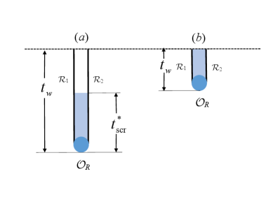
First of all, we consider the region with $t_{w}>t^{*}_{\text{scr}}$, where the process can be illustrated by (a) in Fig.2. In this case, the two time-evolution operators cancel out only during the scrambling time. Then, the complexity can be written as

$\displaystyle C_{\text{pert}}\approx 2\mathcal{R}(t_{w}-t^{*}_{\text{scr}})\,.$

(57)

However, for the case $t_{w}<t^{*}_{\text{scr}}$, as illustrated by (b) in Fig.2, the switchback effect produces a cancellation for the process below the dashed line. Then, the rate of the complexity vanishes.

Summarizing these results, the slope of the complexity of formation can be written as

$\displaystyle\frac{d\Delta C_{\text{pert}}}{dt_{w}}\approx 2\mathcal{R}\mathcal{H}(t_{w}-t^{*}_{\text{scr}})\,.$

(58)

Again, this formula is also in accord with the our holographic case as illustrated in Eqs. (38) and (55) of the last section.

In this paper, we use the CA conjecture to investigate the switchback effect of the TFD state following a quantum quench in the strongly-coupled quantum system with finite $N$ and finite coupling effects. From the viewpoint of the AdS/CFT, this quantum system is dual to a bulk gravitational theory with higher curvature corrections. Then, the investigation is equivalent to studying the switchback effect of the CA complexity in a Vaidya geometry equipped with a light shockwave. Based on the Noether charge formalism of Iyer and Wald, a general expression can be resorting to describing the slope of the complexity of formation in the small and large $t_{w}$ approximations. And the large-time slope of the complexity of formation is essentially twice the late-time growth rate in an unperturbed geometry. By the circuit analogy, we showed this holographic result is essentially in agreement with the switchback effect of the quantum system. The above discussions are independent of the explicit gravitational theory as well as spacetime geometry. This also indicates that the switchback effect is a general feature of the TFD state in the strongly-coupled system with finite $N$ and finite coupling effects. Moreover, according to the calculation of the slope of the complexity, we can see that unlike the late-time complexity growth rate, the countertem will play an important role in the switchback effect.

This research was supported by NSFC Grants No. 11775022 and 11873044.

References

- (1) J. Watrous, “Quantum Computational Complexity,” pp 7174-7201 in Encyclopedia of Complexity and Systems Science, ed., R. A. Meyers (Springer, 2009) quant-ph/0804.3401.
- (2) S. Aaronson, “The Complexity of Quantum States and Transformations: From Quantum Money to Black Holes,” arXiv:1607.05256.
- (3) L. Susskind, “PiTP Lectures on Complexity and Black Holes,” hep-th/1808.09941.
- (4) L. Susskind, “Three Lectures on Complexity and Black Holes,” hep-th/1810.11563.
- (5) L. Susskind,“Computational complexity and black hole horizons,” Fortsch. Phys. 64 24 (2016).
- (6) D. Stanford and L. Susskind, “Complexity and shock wave geometries,” Phys. Rev. D 90, 126007 (2014).
- (7) A. R. Brown, D. A. Roberts, L. Susskind, B. Swingle and Y. Zhao,“Holographic complexity equals bulk action?” Phys. Rev. Lett. 116 191301 (2016).
- (8) A. R. Brown, D. A. Roberts, L. Susskind, B. Swingle and Y. Zhao,“Complexity, action, and black holes,” Phys. Rev. D 93 086006 (2016).
- (9) H. W. Lin and L. Susskind, “Complexity Geometry and Schwarzian Dynamics,” JHEP 2001, 087 (2020).
- (10) L. Susskind, “Complexity and Newton’s Laws,” arXiv:1904.12819.
- (11) A. R. Brown, H. Gharibyan, H. W. Lin, L. Susskind, L. Thorlacius and Y. Zhao, “Complexity of Jackiw-Teitelboim gravity,” Phys. Rev. D 99, 046016 (2019).
- (12) M. Susskind, “Black Holes and Complexity Classes,” arXiv:1802.02175.
- (13) D. A. Roberts, D. Stanford and L. Susskind,“Localized shocks,” JHEP 1503, 051 (2015).
- (14) L.Susskind and Y. Zhao, “Switchbacks and the Bridge to Nowhere,” arXiv:1408.2823.
- (15) Y. Zhao, “A quantum circuit interpretation of evaporating black hole geometry,” arXiv:1912.00909.
- (16) Y. Zhao, “Uncomplexity and Black Hole Geometry,” Phys. Rev. D 97, 126007 (2018).
- (17) Y. Zhao, “Complexity and Boost Symmetry,” Phys. Rev. D 98, no. 8, 086011 (2018).
- (18) A. Bernamonti, F. Galli, J. Hernandez, R. C. Myers, S. M. Ruan and J. Simón, “Aspects of The First Law of Complexity,” arXiv:2002.05779.
- (19) E. Caceres, S. Chapman, J. D. Couch, J. P. Hernandez, R. C. Myers and S. M. Ruan, “Complexity of Mixed States in QFT and Holography,” arXiv:1909.10557.
- (20) A. Bernamonti, F. Galli, J. Hernandez, R. C. Myers, S. M. Ruan and J. Simón, “First Law of Holographic Complexity,” Phys. Rev. Lett. 123, 081601 (2019).
- (21) L.Lehner, R. C. Myers, E. Poisson and R. D. Sorkin, “Gravitational action with null boundaries” Phys. Rev. D 94, 084046 (2016).
- (22) D. Carmi, S. Chapman, H. Marrochio, R. C. Myers and S. Sugishita, “On the time dependence of holographic complexity,” JHEP 1711 188 (2017).
- (23) S. Chapman, H. Marrochio and R. C. Myers, “Complexity of Formation in Holography,” JHEP 1701 062 (2017).
- (24) D. Carmi, R. C. Myers and P. Rath,“Comments on Holographic Complexity,” JHEP 1703 118 (2017).
- (25) Z. Y. Fan and M. Guo, “On the Noether charge and the gravity duals of quantum complexity,” JHEP 1808, 031 (2018).
- (26) AA. Y. Fan and H. Z. Liang,“Time dependence of complexity for Lovelock black holes,” Phys. Rev. D 100, 086016 (2019).
- (27) Z. Y. Fan and M. Guo, “Holographic complexity and thermodynamics of AdS black holes,” Phys. Rev. D 100, 026016 (2019).
- (28) P. A. Cano, R. A. Hennigar and H. Marrochio, “Complexity Growth Rate in Lovelock Gravity,” Phys. Rev. Lett. 121, 121602 (2018).
- (29) P. A. Cano, “Lovelock action with nonsmooth boundaries,” Phys. Rev. D 97, 104048 (2018).
- (30) R. G. Cai, S. He, S. J. Wang and Y. X. Zhang,“Revisit on holographic complexity in two-dimensional gravity,” arXiv:2001.11626.
- (31) K. Nagasaki, “Complexity Growth for Topological Black Holes with a Probe String,” arXiv:1912.03567.
- (32) P. Braccia, A. L. Cotrone and E. Tonni, “Complexity in the presence of a boundary,” JHEP 2002, 051 (2020).
- (33) J. Jiang and H. Zhang, “Surface term, corner term, and action growth in F(Riemann) gravity theory,” Phys. Rev. D 99, 086005 (2019).
- (34) J. Jiang, “Action growth rate for a higher curvature gravitational theory,” Phys. Rev. D 98, 086018 (2018).
- (35) J. Jiang, B. Deng and X. W. Li, “Holographic complexity of charged Taub-NUT-AdS black holes,” Phys. Rev. D 100, 066007 (2019).
- (36) J. Jiang and B. Deng, “Investigating the holographic complexity in Einsteinian cubic gravity,” Eur. Phys. J. C 79 832 (2019).
- (37) J. Jiang and M. Zhang, “Holographic complexity of the electromagnetic black hole,” Eur. Phys. J. C 80, 85 (2020).
- (38) J. Jiang and B. X. Ge, “Investigating two counting methods of the holographic complexity,” Phys. Rev. D 99, 126006 (2019).
- (39) J. Jiang and X. W. Li, “Adjusted complexity equals action conjecture,” Phys. Rev. D 100, 066026 (2019).
- (40) R. Auzzi, G. Nardelli, F. I. Schaposnik Massolo, G. Tallarita and N. Zenoni, “On volume subregion complexity in Vaidya spacetime,” JHEP 1911, 098 (2019).
- (41) S. J. Zhang, “Subregion complexity in holographic thermalization with dS boundary,” Eur. Phys. J. C 79, no. 8, 715 (2019).
- (42) D. Ageev, “Holographic complexity of local quench at finite temperature,” Phys. Rev. D 100, 126005 (2019).
- (43) Y. S. An, R. G. Cai, L. Li and Y. Peng, “Holographic complexity growth in an FLRW universe,” Phys. Rev. D 101, 046006 (2020).
- (44) Y. S. An, R. G. Cai and Y. Peng,“Time Dependence of Holographic Complexity in Gauss-Bonnet Gravity,” Phys. Rev. D 98, 106013 (2018).
- (45) Y. S. An and R. H. Peng, “Effect of the dilaton on holographic complexity growth,” Phys. Rev. D 97, 066022 (2018).
- (46) A. Reynolds and S. F. Ross, Class. “Complexity in de Sitter Space,” Quant. Grav. 34 175013 (2017).
- (47) M. Alishahiha, “Holographic Complexity,” Phys. Rev. D 92 126009 (2015).
- (48) C. A. Agon, M. Headrick and B. Swingle,“Subsystem Complexity and Holography,” arXiv:1804.01561.
- (49) O. Ben-Ami and D. Carmi, “On Volumes of Subregions in Holography and Complexity,” JHEP 1611, 129 (2016).
- (50) Z. Fu, A. Maloney, D. Marolf, H. Maxfield and Z. Wang, “Holographic complexity is nonlocal,” JHEP 1802 072 (2018).
- (51) M. Alishahiha, A. Faraji Astaneh, M. R. Mohammadi Mozaffar and A. Mollabashi, “Complexity Growth with Lifshitz Scaling and Hyperscaling Violation,” JHEP 1807 042 (2018).
- (52) R. Q. Yang, H. S. Jeong, C. Niu and K. Y. Kim, “Complexity of Holographic Superconductors,” JHEP 1904, 146 (2019).
- (53) R. Q. Yang, C. Y. Zhang and W. M. Li,“Holographic entanglement of purification for thermofield double states and thermal quench,” JHEP 1901, 114 (2019).
- (54) R. Q. Yang, C. Niu, C. Y. Zhang and K. Y. Kim, “Comparison of holographic and field theoretic complexities for time dependent thermofield double states,” JHEP 1802, 082 (2018).
- (55) R. Q. Yang, C. Niu and K. Y. Kim, “Surface Counterterms and Regularized Holographic Complexity,” JHEP 1709, 042 (2017).
- (56) S. G. Cai, S. M. Ruan, S. J. Wang, R. Q. Yang and R. H. Peng, “Action growth for AdS black holes,” JHEP 1609, 161 (2016).
- (57) W. J. Pan and Y. C. Huang, “Holographic complexity and action growth in massive gravities,” Phys. Rev. D 95, 126013 (2017).
- (58) W. D. Guo, S. W. Wei, Y. Y. Li and Y. X. Liu, “Complexity growth rates for AdS black holes in massive gravity and gravity,” Eur. Phys. J. C 77, 904 (2017).
- (59) P. Wang, H. Yang and S. Ying, “Action growth in gravity,” Phys. Rev. D 96, 046007 (2017).
- (60) M. Alishahiha, A. Faraji Astaneh, A. Naseh and M. H. Vahidinia, “On complexity for F(R) and critical gravity,” JHEP 1705, 009 (2017).
- (61) J. Couch, S. Eccles, W. Fischler and M. L. Xiao,“Holographic complexity and noncommutative gauge theory,” JHEP 1803 108 (2018).
- (62) B. Swingle and Y. Wang, “Holographic Complexity of Einstein-Maxwell-Dilaton Gravity,” JHEP 1809 106 (2018).
- (63) A.P. Reynolds and S. F. Ross, “Complexity of the AdS Soliton,” Class. Quant. Grav. 35 095006 (2018).
- (64) R. Nally, “Stringy Effects and the Role of the Singularity in Holographic Complexity,” JHEP 1909, 094 (2019).
- (65) S.Chapman, H. Marrochio and R. C. Myers, JHEP “Holographic complexity in Vaidya spacetimes. Part I,” 1806 046 (2018).
- (66) S. Chapman, H. Marrochio and R. C. Myers, “Holographic complexity in Vaidya spacetimes. Part II,” JHEP 1806 114 (2018).
- (67) Z. Y. Fan and M. Guo, “Holographic complexity under a global quantum quench,” Nucl. Phys. B 950, 114818 (2020).
- (68) J. Jiang, “Holographic complexity in charged Vaidya black hole,” Eur. Phys. J. C 79 130 (2019).
- (69) B. Chen, W. M. Li, R. Q. Yang, C. Y. Zhang and S. J. Zhang, “Holographic subregion complexity under a thermal quench,” JHEP 1807, 034 (2018).
- (70) R. Auzzi, G. Nardelli, F. I. Schaposnik Massolo, G. Tallarita and N. Zenoni, “On volume subregion complexity in Vaidya spacetime,” JHEP 1911, 098 (2019).
- (71) M. Reza Tanhayi, R. Vazirian and S. Khoeini-Moghaddam,“Complexity Growth Following Multiple Shocks,” Phys. Lett. B 790, 49 (2019).
- (72) M. Moosa, “Evolution of Complexity Following a Global Quench,” JHEP 1803, 031 (2018).
- (73) M. Nozaki, T. Numasawa and T. Takayanagi, “Holographic Local Quenches and Entanglement Density,” JHEP 1305, 080 (2013).
- (74) P. Caputa, J. Simon, A. Stikonas, and T. Takayanagi, “Quantum entanglement of localized excited states at finite temperature,” JHEP. 01, 102 (2015).
- (75) M. M. Roberts, “Time evolution of entanglement entropy from a pulse,” JHEP 1212, 027 (2012).
- (76) A. F. Astaneh and A. E. Mosaffa, “Holographic Entanglement Entropy for Excited States in Two Dimensional CFT,” JHEP 1303, 135 (2013).
- (77) C. T. Asplund and A. Bernamonti, “Mutual information after a local quench in conformal field theory,” Phys. Rev. D 89 066015 (2014).
- (78) S. Lloyd, “Ultimate physical limits to computation,” Nature (London) 406 (Aug., 2000)
- (79) D. S. Ageev, I. Y. Aref’eva, A.A. Bagrov, and M. I. Katsnelson, “Holographic local quench and effective complexity,” JHEP 1808, 071 (2018).
- (80) D. Ageev, Holography, “quantum complexity and quantum chaos in different models,” EPJ Web Conf. 191, 06006 (2018).
- (81) D. Ageev, “Holographic complexity of local quench at finite temperature,” Phys. Rev. D 100, 126005 (2019).
- (82) J. Abajo-Arrastia, J. Aparicio and E. Lopez, “Holographic Evolution of Entanglement Entropy,” JHEP 1011, 149 (2010).
- (83) V. Balasubramanian et al., “Thermalization of Strongly Coupled Field Theories,” Phys. Rev. Lett. 106, 191601 (2011)
- (84) V. Balasubramanian, A. Bernamonti, N. Copland, B. Craps and F. Galli, “Thermalization of mutual and tripartite information in strongly coupled two dimensional conformal field theories,” Phys. Rev. D 84, 105017 (2011).
- (85) A. Allais and E. Tonni, “Holographic evolution of the mutual information,” JHEP 1201, 102 (2012).
- (86) T. Hartman and J. Maldacena, “Time Evolution of Entanglement Entropy from Black Hole Interiors,” JHEP 1305 014 (2013)
- (87) H. Liu and S. J. Suh, “Entanglement growth during thermalization in holographic systems,” Phys. Rev. D 89, 066012 (2014).
- (88) C. T. Asplund and A. Bernamonti, “Mutual information after a local quench in conformal field theory,” Phys. Rev. D 89, 066015 (2014).
- (89) V. Ziogas, “Holographic mutual information in global Vaidya-BTZ spacetime,” JHEP 1509, 114 (2015).
- (90) J. Jiang, J. Shan and J. Yang, “Circuit complexity for free Fermion with a mass quench,” arXiv:1810.00537.
- (91) J. Jiang and X. Liu, “Circuit Complexity for Fermionic Thermofield Double states,” Phys. Rev. D 99, 026011 (2019).
- (92) R. A. Jefferson and R. C. Myers, “Circuit complexity in quantum field theory,” JHEP 1710 107 (2017).
- (93) M. Guo, J. Hernandez, R. C. Myers and S. M. Ruan, “Circuit Complexity for Coherent States,” JHEP 1810 011 (2018).
- (94) S. Chapman, J. Eisert, L. Hackl, M. P. Heller, R. Jefferson, H. Marrochio and R. C. Myers, “Complexity and entanglement for thermofield double states,” SciPost Phys. 6, 034 (2019).
- (95) L. Hackl and R. C. Myers, “Circuit complexity for free fermions,” JHEP 1807 139 (2018).
- (96) R. Q. Yang, Y. S. An, C. Niu, C. Y. Zhang and K. Y. Kim, “To be unitary-invariant or not?: a simple but non-trivial proposal for the complexity between states in quantum mechanics/field theory,” arXiv:1906.02063.
- (97) R. Q. Yang, Y. S. An, C. Niu, C. Y. Zhang and K. Y. Kim, “More on complexity of operators in quantum field theory,” JHEP 1903, 161 (2019)
- (98) R. Q. Yang, Y. S. An, C. Niu, C. Y. Zhang and K. Y. Kim, “Principles and symmetries of complexity in quantum field theory,” Eur. Phys. J. C 79, no. 2, 109 (2019)
- (99) R. Q. Yang,“Complexity for quantum field theory states and applications to thermofield double states,” Phys. Rev. D 97, 066004 (2018).
- (100) S.Khan, C. Krishnan, and S. Sharma, “Circuit Complexity in Fermionic Field Theory,” Phys. Rev. D 98, 126001 (2018).
- (101) T. Chapman and H. Z. Chen, “Complexity for Charged Thermofield Double States,” arXiv:1910.07508.
- (102) M. Doroudiani, A. Naseh and R. Pirmoradian, “Complexity for Charged Thermofield Double States,” JHEP 2001, 120 (2020).
- (103) S. Chapman, M. P. Heller, H. Marrochio and F. Pastawski,“ Towards Complexity for Quantum Field Theory States” Phys. Rev. Lett. 120, 121602 (2018).
- (104) V. Iyer and R.M. Wald, “Some properties of Noether charge and a proposal for dynamical black hole entropy,” Phys. Rev. D 50, 846 (1994).
- (105) J. M. Maldacena, “Eternal black holes in anti-de Sitter,” JHEP 0304, 021 (2003).
- (106) R. C. Myers and M. J. Perry, “Black Holes in Higher Dimensional Space-Times,” Annals Phys. 172, 304 (1986).
- (107) C. Bambi and L. Modesto, “Rotating regular black holes,” Phys. Lett. B 721, 329 (2013).
- (108) J. P. S. Lemos and V. T. Zanchin, “Rotating charged black string and three-dimensional black holes,” Phys. Rev. D 54, 3840 (1996).
- (109) J. W. Moffat,“Black Holes in Modified Gravity (MOG),” Eur. Phys. J. C 75, 175 (2015).
- (110) A. Sen,“Rotating charged black hole solution in heterotic string theory,” Phys. Rev. Lett. 69, 1006 (1992).
- (111) N. Alonso-Alberca, P. Meessen and T. Ortin, “Supersymmetry of topological Kerr-Newman-Taub–NUT-AdS space-times,” Class. Quant. Grav. 17, 2783 (2000).
- (112) D. L. Wiltshire, Spherically symmetric solutions of Einstein-Maxwell theory with a Gauss-Bonnet term, Phys. Lett. 169B, 36 (1986).
- (113) J. C. S. Neves and C. Molina, “Rotating black holes in a Randall-Sundrum brane with a cosmological constant,” Phys. Rev. D 86, 124047 (2012).
- (114) J. B. Griffiths and J. Podolsky, “A new look at the PlebanskiDemianski family of solutions,” Int. J. Mod. Phys. D 15, 335 (2006).
- (115) W. Kim, S. Kulkarni and S. H. Yi, “Quasilocal Conserved Charges in a Covariant Theory of Gravity,” Phys. Rev. Lett. 111 081101 (2013).