Surrogate distributed radiological sources III: quantitative distributed source reconstructions
Abstract
In this third part of a multi-paper series, we present quantitative image reconstruction results from aerial measurements of eight different surrogate distributed gamma-ray sources on flat terrain. We show that our quantitative imaging methods can accurately reconstruct the expected shapes, and, after appropriate calibration, the absolute activity of the distributed sources. We conduct several studies of imaging performance versus various measurement and reconstruction parameters, including detector altitude and raster pass spacing, data and modeling fidelity, and regularization type and strength. The imaging quality performance is quantified using various quantitative image quality metrics. Our results confirm the utility of point source arrays as surrogates for truly distributed radiological sources, advancing the quantitative capabilities of Scene Data Fusion gamma-ray imaging methods.
Index Terms:
gamma-ray imaging, distributed sources, airborne survey, image reconstructionI Introduction
As described in Parts I [1] and II [2] of this multi-paper series, we designed, fielded, and measured surrogate distributed radiological sources constructed from arrays of up to Cu-64 point sources. In this Part III, we finally turn to the task of quantitatively imaging these distributed sources, i.e., determining both the shape and magnitude of radiation intensities in the mapped area.
Quantitative distributed source image reconstruction represents an advance in complexity compared to the two more common distributed source mapping modalities, namely either simply measuring dose rates at multiple points and interpolating between them (“breadcrumbing”), or performing only qualitative, relative “hot” vs. “cold” reconstructions with no absolute scale. This increase in complexity, however, provides an additional wealth of information that may be used to drive decision-making, such as whether a radionuclide concentration in the environment is above regulatory limits, or how to minimize the dose to personnel at ground level based on aerial measurements.
In addition to Parts I and II, this paper builds upon much of our previous work demonstrating free-moving quantitative gamma-ray imaging of small ( m2) distributed sources [3], and is part of a larger effort in advancing the quantitative capabilities of a radiation mapping technique we have termed “Scene Data Fusion” (SDF) [4], which leverages contextual sensors to describe the image space to which measured radiation is attributed. Distributed source mapping has also been of interest to several other groups concerned with radiological emergency response—see for instance Refs. [5, 6, 7, 8]. This paper in particular offers a number of contributions over existing work. First, while the state of the art often uses traditional Compton imagers or passive coded mask imagers, both of which typically have a limited field of view, this work focuses on singles (i.e., non-Compton) imaging with omnidirectional gamma-ray imagers. Second, compared to the existing literature (which, again, often produces only qualitative, relative-scale images), the well-known configuration of the point source arrays allow us to make more thorough quantitative comparisons between the reconstructed images and the ground truth configurations. Third, due to the reconfigurability of the array sources, we were able to measure a number of distributed source patterns of varying complexity, offering a more comprehensive study of various intensity and spatial features. Finally, we also investigate quantitative reconstruction performance for a wide variety of experiment and reconstruction parameters.
The paper structure is as follows: Section II provides an overview of the measurement campaign, quantitative reconstruction methods used, and image quality metrics chosen. Section III then provides quantitative reconstruction results in a number of studies. In particular, we show sample imaging results for the eight distributed source types using representative flight parameters and reconstruction hyper-parameters, and then perform sweeps over various (hyper-)parameters such as detector altitude and regularization strength. Sections IV and V then conclude with a further discussion of results and a general summary of findings.
II Methods
II-A Measurement overview
As described in Part II [2], in August 2021 we conducted a week-long experimental campaign at Washington State University (WSU) using radiation detectors borne on unmanned aerial systems (UASs) to measure the gamma-ray signature of various surrogate distributed Cu-64 source patterns. The source patterns were constructed out of arrays of up to point sources spaced densely enough to “look like” a truly continuous distributed source of Cu-64 for a given detector and trajectory (according to the method developed in Part I, Section II), and range in complexity from a uniform square source to regions of higher and zero activity superimposed on a uniform baseline (see Part I, Fig. 3). The nominal point source activities were mCi at 0800 PDT of each measurement day, though the sources decayed throughout the day with a -hour half-life, and the count rate comparisons made in Part II Section V-A suggest that the true source activities were higher than the planned nominal activities, which were subject to substantial calibration uncertainties. In this work, we consider this scale factor to be part of the overall system calibration. The predominant decay signature of Cu-64 is the keV annihilation photon line, which can be detected either in ‘singles’ mode (i.e., through its photopeak) or in ‘doubles’ mode (i.e., through its Compton scattering between two detector segments). In this work, we restrict ourselves to singles imaging, but note that Compton imaging analyses remains of interest. The detector systems used are NG-LAMP ( CLLBC modules) [9] and MiniPRISM ( CZT modules) [10], both of which are capable of omnidirectional gamma-ray imaging. Due to the imperfect energy resolution of real detectors, we define the energy region of interest (ROI) corresponding to the keV photopeak to be keV for NG-LAMP and keV for MiniPRISM—see Part II. Also as described in Part II, when necessary we exclude data from detector crystals that regularly exhibited poor spectral and/or timing performance throughout the campaign. As such, NG-LAMP crystals and MiniPRISM crystals were used for these analyses. Finally, we restrict our analysis to data collected during the constant-altitude UAS raster patterns, i.e., we exclude takeoff/landing and any other free-form trajectories performed.
II-B Scene generation and co-registration
To make detailed quantitative comparisons between the distributed sources designed in Part I and their SDF reconstructions, accurate models of the measured scene must be generated and then aligned with the designed coordinate frame to as good a precision as possible.
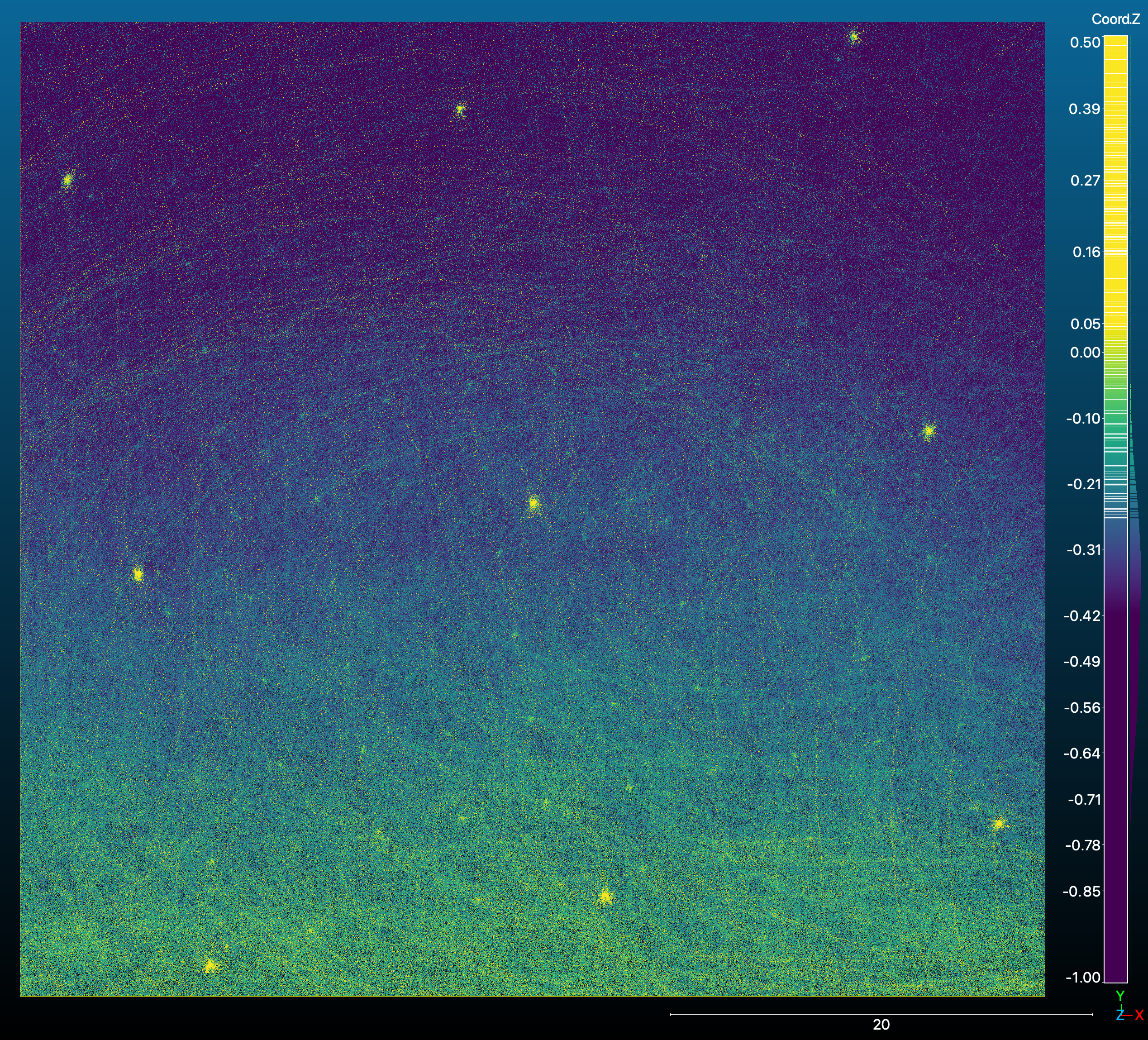
The NG-LAMP and MiniPRISM detector systems are each equipped with a lidar and inertial measurement unit (IMU) to enable lidar-based simultaneous localization and mapping (SLAM) [11, 12] in order to reconstruct the detector trajectory and a 3D digital point cloud model of the mapped area. To co-register all SLAM results to the idealized field coordinate frame used in Part I, we first identified a high-quality SLAM map of a square source run in which most of the individual source locations were resolvable. The field had a slope of for drainage, so we then aligned the field normal to the axis by fitting a small plane near the center of the square source. After the point cloud was leveled, we were able to identify of the source locations through manual inspection in the CloudCompare software, and imputed a constant source position based on the apparent ground surface within the point cloud. These lidar source position estimates were then aligned with their corresponding points in the ideal square source (of exactly m grid spacing) using a least-squares distance minimization between all corresponding point sets, and the resulting transformation was applied to the leveled point cloud. The mean distance between the designed and lidar source points after co-registration was cm (with the mean - and -component differences 1 mm), and the mean grid spacing between the lidar source points was m, only different from the design value of m. Fig. 1 shows the lidar point cloud colorized by height and the positions of the discernible square source locations after alignment.

The remaining point clouds were then co-registered to the now-aligned reference cloud using the Iterative Closest Point (ICP) algorithm in Open3D [13]. We enforced a minimum ICP fitness score of (chosen empirically), and manually provided improved initial guesses for the transform if the initial ICP result did not meet this threshold on the first pass. Fig. 2 shows the results of this co-registration procedure on point clouds from the campaign. Finally, after all measurements were co-registered, the volume for radiological source reconstruction was defined as the plane m at , with a m pixel size.


II-C Image reconstruction
As described in Part I Section II-A, we perform single-energy gamma-ray imaging by assuming a linear model
| (1) |
where is the vector of gamma-ray intensities or “weights” at each point or voxel center indexed , is the vector of expected counts observed by a detector over a series of measurements indexed , is the system matrix that relates the weights to the expected counts, and the subscript denotes non-negativity. An unknown but constant-in-time background term, , can also be included and solved for (see Ref. [3]), but we exclude it in this discussion for clarity and because our measurements are heavily source-dominated. The element of the system matrix is
| (2) |
where is the effective area to source point during measurement (e.g., Fig. 5(a) of Ref. [3]), is the corresponding distance vector, and is the dwell time. A measurement (or series thereof) consists of a Poisson sample
| (3) |
which has a corresponding Poisson negative log-likelihood of
| (4) |
where denotes element-wise multiplication. Eq. 4 can also be used in defining the “unit deviance” or “deviance residual” between the data and the model, which reduces to a metric at high counts—see Part I, § II-D.
A maximum likelihood radiation image reconstruction algorithm then seeks the optimization
| (5) |
or, by incorporating prior information, a maximum a posteriori algorithm seeks
| (6) |
for some hyperparameter and regularization function , which are often chosen to promote sparseness and/or smoothness in the reconstructed image . Eq. 5 can be solved iteratively through the maximum likelihood expectation maximization (ML-EM) algorithm [14, 15]
| (7) |
where is typically initialized to a flat image and the sensitivity map
| (8) |
describes the expected number of counts per unit weight for each source element summed over the measurements. Moreover Eq. 7 can be extended to solve the regularized minimization in Eq. 6 (“maximum a posteriori expectation maximization” or MAP-EM)—see Ref. [3], Eqs. 7–8 for further details. In particular we consider the sparsity-promoting, non-convex prior [16],
| (9) |
and the smoothing and edge-preserving total variation (TV) prior [17, 18], which can be written in 2D as
| (10) |
Computationally, the integrals in Eq. 10 are replaced with discrete sums and the derivatives with finite differences. An additional parameter is often introduced to stabilize calculations when taking the gradient of Eq. 10 [18, §II-C]. Reconstruction algorithms are implemented in the mfdf [19] package using radkit libraries [20], and run on a graphics processing unit (GPU) via PyOpenCL.
II-D Image quality metrics
To evaluate the quality of a reconstructed radiation image compared to its corresponding ground truth image , we will typically consider three metrics: (1) the ratio of total reconstructed and true activities,
| (11) |
(2) the normalized root-mean-square error (NRMSE),
| (12) |
and (3) the structure coefficient from Eq. 10 of Ref. [21],
| (13) |
for some small stabilizing constant . We note that the structure coefficient, , is essentially the Pearson correlation coefficient between the image pixel intensities. The activity ratio, , is chosen to give an overall intensity accuracy (closer to is better), the NRMSE is chosen to measure the average intensity similarity over the image independent of pixel position and normalized by the true total (closer to is better), and the structure metric, , is chosen to measure perceived image similarity (closer to is better). In Figs. 3, 4, 7–10, and 12–14, these metrics are displayed on each reconstructed activity image.
Because the on-field source distributions consisted of individual point sources specifically configured to emulate continuous distributed sources, for the purposes of quantitative image comparison the “true” images are generated by interpolating the point source arrays to -m pitch continuous ground truth images with the same average activity concentrations.
While reconstructed images are computed over the entire field, much of that area has zero source present, and, as shown in Section III, correspondingly quite low reconstructed activity compared to the areas with source present. Thus, to reduce the extent to which image quality metrics are dominated by near-zero comparisons, we compute the image quality metrics over smaller subsets of the image space. In particular, we compute the NRMSE using only pixels with non-zero activity in the interpolated ground truth distributions, and compute the structure metric in the domain m.
III Results
III-A Image study
Figs. 3 and 4 show radiation image reconstruction results from eight different source measurements with the NG-LAMP system at a nominal m above ground level (AGL), a raster pass spacing of m, and a speed of m/s. Binmode MAP-EM reconstructions with a time binning of s were performed in a 2D image plane of dimensions with pixels, and ran in – s on a 2019 MacBook Pro using an AMD Radeon Pro 5600M 8 GB GPU. Here we use the sparsity-promoting regularizer with coefficient and iterations, which are useful representative values chosen manually based on our prior reconstruction experience. We note however that we explore the impact of these regularization parameters, as well as many of the other measurement parameters, in the subsequent sections. We also note that in Figs. 3, 4, and many subsequent image reconstruction figures, the measured trajectories are overlain and colorized by gross count rates (the aforementioned breadcrumbing approach) with a cyan-to-magenta color scale as a qualitative, additional guide, without showing explicit quantitative colorbars. In general, though, the gross count rates in these figures are s far from the source and as high as s above high activity concentration areas and/or sources measured early in the day. Both trajectories and point source array distributions are shown when their inclusion is relevant and they can be overlain without compromising the clarity of the reconstructed image.


In general, the reconstructions accurately map the shape and, after calibration, the magnitude of the ground truth radiation distributions. Some overall differences in activity distribution are notable, however. The interior activities of the shapes are generally over-predicted compared to ground truth, while the edges are under-predicted. In addition, the corners and edges of the reconstructed images are rounded compared to the sharp features of the true images, falling off smoothly over a few meters rather than instantly over a m pixel. As a result, the zero-activity corridor is not very sharp in the m separation reconstruction, though it is better-resolved in the m separation reconstruction. Quantitatively, the ratios of total reconstructed activity range from ( m separation) to (plume), indicating high precision and a slight – bias in the absolute magnitude of the source reconstructions. The NRMSE ranges from (hot/coldspot) to ( m separation), indicating fairly good average shape agreement despite the smoother nature of the reconstructed images. Finally, the structure coefficient ranges from ( m separation) to ( square), indicating a high level of perceived shape similarity.
For additional context, Fig. 5 compares the measured and MAP-EM-reconstructed counts vs. time from the square source reconstruction of Fig. 3. The deviance residuals and smoothness of the MAP-EM curve qualitatively indicate that the MAP-EM algorithm is not overfitting to noise, and thus that iterations is a suitable choice in this scenario. For an example energy spectrum, see Fig. 5 of Part II. Finally, Fig. 6 shows a 3D render of the measurement and reconstruction.


III-B Altitude study
Fig. 7 shows the results from a series of measurements in which the NG-LAMP system was flown over the m separation source at altitudes of , , , and m AGL in order to observe trends in the reconstruction vs. detector altitude. All three performance metrics degrade monotonically with increasing altitude. The structure coefficient in particular falls from to and the sum ratio decreases from to between m and m AGL.

These trends confirm that in the idealized case of an omnidirectional radiation detector flying over a flat plane with no intervening material, there is no imaging advantage in flying higher, as opposed to a traditional optical camera where the size of the viewed area increases with altitude. In real measurement scenarios, there are of course operational advantages to higher altitudes, in particular, the avoidance of obstacles that may attenuate the radiation signal and pose a collision risk for UASs.
III-C Replication study
Fig. 8 demonstrates the reproducibility of the method, where the NG-LAMP system was flown over the square source at m AGL in four runs between approximately and PDT on the same day. The three performance metrics are remarkably consistent (less than a few percent variation) run-to-run, despite small variations in the measured trajectory and the decay of the Cu-64 sources ( hours), both of which are visible in the images.

III-D Coarse-graining study
Fig. 9 shows the results of an analysis of data where the MiniPRISM system was flown over the m-separation source at a nominal m AGL and the fidelities of both the data and detector response models were progressively coarsened. In particular, the data were re-sampled from the original s to s and s dwell times, and the detector response was degraded from its initial anisotropic multi-crystal response to a single isotropic detector with the same total effective area . The coarsening of the response to an isotropic detector has only a small negative effect on the reconstruction performance; this is not surprising as the modulation of the counts in Eq. 2 is much stronger than the modulation for these airborne surveys. For further exploration of the negative effect of response coarsening on reconstruction performance, we refer the reader to Ref. [22]. The coarsening of the data to - or -s intervals, conversely, slightly and then significantly degrades reconstruction performance. While the degradation to s is small according to the three performance metrics, the shape of the distribution noticeably degrades by eye, with the two rectangular activity bands smearing towards the center of the image. At s, the degradation is even more substantial, with prominent activity smearing (concentrated near the trajectory points) and corresponding changes in the NRMSE and structure metrics.

III-E Speed study
Similar to the coarse-graining study of Fig. 9, Fig. 10 shows reconstruction results for the m-separation source with MiniPRISM at m AGL as the UAS flight speed is increased. Although during measurements only a single speed of m/s was set, we emulate faster speeds by downsampling the listmode radiation data and compressing the radiation and trajectory timestamps by a constant factor. In particular, Fig. 10 shows effective speed increases of , , , and , resulting in emulated speeds of , , , and m/s, and corresponding total measurement times of , , , and s. Note that we maintain a constant readout interval of s, unlike the coarse-graining study, and thus the baseline reconstruction in Fig. 10 differs slightly from the baseline reconstruction in Fig. 9.

As the speed of the UAS raster increases, the reconstruction noise increases and the image quality decreases due to the reduction in photon statistics. Fig. 11 shows the image quality metrics at more speeds than Fig. 10. While the image quality does not markedly decrease at a speedup ( m/s), the NRMSE rises from the baseline to at the speedup ( m/s), suggesting a top speed of m/s is suitable for this particular mapping scenario. Fig. 11 also suggests that the NRMSE and structure metrics are strongly anti-correlated.

III-F Regularizer studies
Fig. 12 shows the results of a series of analyses of a single data collection where the NG-LAMP system was flown at m AGL above the -shape source, and the regularizer coefficient and number of iterations were varied between relatively low and high values— vs. and vs. , respectively. In all four cases, the overall -shape is correctly observed, but at various levels of sharpness and thus agreement with the true distribution. The image is over-regularized, producing a distribution that is significantly smaller than the true source distribution, and has a correspondingly high NRMSE of and low structure coefficient of . At the other end of the spectrum, the image has not fully converged, resulting in a modest NRMSE of but an improved structure coefficient of . The intermediate case of the image performs the best of the four combinations, with an NRMSE of , a structure coefficient of , and a sum ratio of . This hyperparameter selection even slightly outperforms the initial hyperparameters used for the -shape reconstruction in Fig. 3, which had an NRMSE of , a structure coefficient of , and a sum ratio of . Therefore we note again that the question of rigorous optimal hyperparameter selection based on comparison to ground truth is left for future work.

Fig. 13 shows the results of a second regularizer study in which NG-LAMP was flown at m AGL over the hot/coldspot source, and the TV regularizer coefficient and number of iterations were varied from to and to , respectively, while using a fixed s as per Ref. [18, §II-C]. The upper bound of the regularizer coefficient was kept lower than the regularizer study, and the final two image iterations were averaged together, in order to avoid inducing strong “checkerboard” image artifacts that oscillate every iteration at . Such checkerboard artifacts appear to be a limitation of the TV regularizer at relatively high arising from the fact that minimizing finite differences in and smooths the horizontal and vertical bands of the image, but does not constrain diagonally-adjacent pixels [23]. We also note that for computational tractability, these reconstructions use data summed over all NG-LAMP detector crystals. Both images using iterations appear under-converged, with some apparent blurring between the three hot, cold, and baseline regions. After iterations, the hot and coldspots become more distinct from the uniform baseline, with the image outperforming the image in terms of NRMSE and structure coefficient. In all four TV-regularized images, the summed activity ratio is in general closer than images using the regularizer by about , though the reason for this is not readily apparent, and similarly the NRMSE values are lower by up to . Further discussion of the TV vs regularizer performance is given in Section IV.

III-G Raster spacing study
Fig. 14 shows the results of another series of analyses from a single data collection in which NG-LAMP was flown at m AGL over the -shape source using a tighter-than-normal line-spacing of m (instead of m) to facilitate testing trajectory cuts in post-processing. In particular, we cut the trajectory into individual raster lines by simple timestamp cuts and then perform reconstructions (both unregularized and with the standard ) using only every raster line for .

The correct shape of the -shape source is visible for but the shape severely degrades for . The degradation is more severe in the -regularized reconstructions due to the sparsity-promoting nature of the regularizer. These trends are borne out by the overall drop in structure coefficient from at to at (regularized) and from to (unregularized), and the corresponding increase in NRMSE from to (regularized) and to (unregularized). For reference, Fig. 14 also shows the sensitivity maps for each post-cut measurement. The worst-performing images are associated with sensitivity maps that contain noticeable visual banding between the raster lines, indicating that achieving uniform sensitivity over the source area improves quantitative reconstruction. A similar line of reasoning can also be used to argue that some non-trivial amount of measurement time should be spent flying over source-free areas in order to better capture the contrast between signal and background, though we do not take up this question quantitatively here.
IV Discussion
The results of Section III have shown good reconstruction quality, both by eye and by our quantitative image metrics, when the reconstruction hyper-parameters are sensibly chosen. In this Section, we discuss how these datasets may be leveraged to further advance quantitative radiation imaging.
Through the altitude, coarse-graining, speed, and raster spacing studies, we have explored whether specific datasets are sufficient for high-quality reconstructions. While we are able to investigate trends in image quality metrics through these somewhat brute-force parameter sweeps, we expect that information-theory-based approaches may offer additional insights. An improved understanding of data sufficiency could help both in designing efficient distributed sources experiments, and in determining (perhaps autonomously in real-time) what regions to map and for how long. Such questions have been explored in the single- or few-point-source case (e.g., Refs. [24, 25]) but to our knowledge have only recently begun to be explored for fully-distributed sources [26]. Similarly, notions such as the matrix condition number may be useful in exploring the underdeterminedness of the linear model of Eq. 1, though computing the condition number for high-dimensional models remains a computational challenge.
The coarse-graining, speed, and raster spacing studies also demonstrate the capability to resample the dense measured data in post-processing in order to emulate mapping with different detector trajectories. Because the change in source activity due to radioactive decay during a given measurement is small ( over a minute flight), in future work we may arbitrarily rearrange data in time within the measurement to test, for instance, autonomous trajectory planning methods.
Although we have performed some MAP-EM regularizer studies via Figs. 12 and 13, as discussed above we leave a more thorough study of hyperparameter optimization for future work. As the optimal hyperparameters appear to vary with altitude, system, source, and regularizer type, such an intensive study is beyond the scope of the present paper. Such a study could also make use of more advanced stopping criteria (e.g., Refs. [27, 28, 29]) compared to the pre-set number of iterations (typically ) used here.
Although the TV regularizer may seem like the natural candidate for all source distributions in this work, here we prefer the regularizer for several reasons. First, the regularizer uses only one free parameter (the regularization strength ) while the TV regularizer uses a strength and a stabilization coefficient . While Ref. [18, §II-C] gives a suggestion on how set , it depends on the image itself, necessitating a manual iterative tuning process. Also, as noted in Section III-F, the TV regularizer can induce checkerboard image artifacts that necessitate a somewhat ad hoc averaging of two image iterations. More generally, it is valuable to explore the regularizer since it is expected to improve reconstructions for both plume-like and sharp-edged source distributions, while the TV regularizer will be of limited utility for the former.
Uncertainty quantification (UQ) for these distributed source reconstructions also remains a topic of ongoing work, especially since it will require computationally-tractable high-dimensional UQ methods to compute uncertainties for all image pixels. The replication study however already indicates a high degree of precision (which suggests a low systematic uncertainty) in reconstructing measurements when holding all parameters constant (other than the decay of the Cu-64 source throughout the day).
Finally, as noted in Part II [2], in September 2023 we conducted a second distributed sources mapping campaign at the Johns Hopkins Applied Physics Laboratory (JHU APL) using mCi Cs-137 point-like sources on hilly terrain. Analysis of this data is underway and preliminary results are quite promising in terms of quantitative reconstruction accuracy; in particular, there is no need for the activity calibration factor used for the present WSU Cu-64 measurements. These results will also be presented in future work. We also anticipate testing Compton reconstruction modes on some of the JHU APL source distributions, though our singles-mode design assumption in Part I [1] will not apply, and thus the sources may no longer appear continuous.
V Conclusion
We have performed quantitative reconstructions of surrogate distributed radiological sources as measured by airborne gamma-ray spectrometers. In general, our reconstructions accurately reconstruct the expected source shapes both by eye and as measured by various quantitative performance metrics. The absolute activity scale can also be determined to within after applying the activity calibration developed in Part II. We also performed various parameter sweeps, analyzing reconstruction performance vs. detector altitude and speed, detector response coarsening, data coarsening, and regularizer type and hyperparameters. In the -Ci-scale, -m2-extent examples here, performance degraded significantly at altitudes above m, at line spacings above m, or at speeds above m/s, suggesting that keeping UAS flight parameters within these bounds is necessary for high-quality reconstructions. Conversely, in this aerial mapping modality, detector response fidelity had a minimal impact on reconstruction performance, with the full anisotropic response models performing only marginally better than their equivalent isotropic models. We also investigated the impact of two different regularization methods ( and TV), determined suitable (though not yet optimal) hyperparameters for each, and showed that both are capable of producing high-quality reconstructed images. More broadly, this work confirms the feasibility of using point source arrays as surrogate distributed sources for distributed source imaging studies, benchmarks LBNL’s quantitative Scene Data Fusion (SDF) capabilities for reconstructing distributed sources, and provides a useful dataset and framework for further studies.
Acknowledgements
We thank the students and staff of the Washington State University Nuclear Science Center for their assistance in moving sources and general experimental logistics during the measurement campaign.
This material is based upon work supported by the Defense Threat Reduction Agency under HDTRA 13081-36239. This support does not constitute an express or implied endorsement on the part of the United States Government. Distribution A: approved for public release, distribution is unlimited.
This document was prepared as an account of work sponsored by the United States Government. While this document is believed to contain correct information, neither the United States Government nor any agency thereof, nor the Regents of the University of California, nor any of their employees, makes any warranty, express or implied, or assumes any legal responsibility for the accuracy, completeness, or usefulness of any information, apparatus, product, or process disclosed, or represents that its use would not infringe privately owned rights. Reference herein to any specific commercial product, process, or service by its trade name, trademark, manufacturer, or otherwise, does not necessarily constitute or imply its endorsement, recommendation, or favoring by the United States Government or any agency thereof, or the Regents of the University of California. The views and opinions of authors expressed herein do not necessarily state or reflect those of the United States Government or any agency thereof or the Regents of the University of California.
This manuscript has been authored by an author at Lawrence Berkeley National Laboratory under Contract No. DE-AC02-05CH11231 with the U.S. Department of Energy. The U.S. Government retains, and the publisher, by accepting the article for publication, acknowledges, that the U.S. Government retains a non-exclusive, paid-up, irrevocable, world-wide license to publish or reproduce the published form of this manuscript, or allow others to do so, for U.S. Government purposes.
This research used the Lawrencium computational cluster resource provided by the IT Division at the Lawrence Berkeley National Laboratory (Supported by the Director, Office of Science, Office of Basic Energy Sciences, of the U.S. Department of Energy under Contract No. DE-AC02-05CH11231).
References
- [1] Jayson R Vavrek, Mark S Bandstra, Daniel Hellfeld, Brian J Quiter, and Tenzing HY Joshi. Surrogate distributed radiological sources I: point-source array design methods. IEEE Transactions on Nuclear Science, 2024.
- [2] Jayson R Vavrek, C Corey Hines, Mark S Bandstra, Daniel Hellfeld, Maddison A Heine, Zachariah M Heiden, Nick R Mann, Brian J Quiter, and Tenzing HY Joshi. Surrogate distributed radiological sources II: aerial measurement campaign. IEEE Transactions on Nuclear Science, 2024.
- [3] D Hellfeld, MS Bandstra, JR Vavrek, DL Gunter, JC Curtis, M Salathe, R Pavlovsky, V Negut, PJ Barton, JW Cates, et al. Free-moving quantitative gamma-ray imaging. Scientific reports, 11(1):1–14, 2021.
- [4] Kai Vetter, Ross Barnowski, Joshua W Cates, Andrew Haefner, Tenzing HY Joshi, Ryan Pavlovsky, and Brian J Quiter. Advances in nuclear radiation sensing: Enabling 3-D gamma-ray vision. Sensors, 19(11):2541, 2019.
- [5] NJ Murtha, LE Sinclair, PRB Saull, A McCann, and AML MacLeod. Tomographic reconstruction of a spatially-extended source from the perimeter of a restricted-access zone using a SCoTSS compton gamma imager. Journal of Environmental Radioactivity, 240:106758, 2021.
- [6] A MacLeod, N Murtha, P Saull, L Sinclair, and M Andrew. 3-D reconstruction of extended sources during dispersal trial with a Compton imager. In 2023 IEEE Nuclear Science Symposium, Medical Imaging Conference and International Symposium on Room-Temperature Semiconductor Detectors (NSS MIC RTSD). IEEE, 2023.
- [7] CG Wahl, R Sobota, and D Goodman. 3D Compton mapping of point and distributed sources with moving detectors. In 2023 IEEE Nuclear Science Symposium, Medical Imaging Conference and International Symposium on Room-Temperature Semiconductor Detectors (NSS MIC RTSD). IEEE, 2023.
- [8] G Daniel and O Limousin. Extended sources reconstructions by means of coded mask aperture systems and deep learning algorithm. Nuclear Instruments and Methods in Physics Research Section A: Accelerators, Spectrometers, Detectors and Associated Equipment, 1012:165600, 2021.
- [9] R Pavlovsky, JW Cates, WJ Vanderlip, THY Joshi, A Haefner, E Suzuki, R Barnowski, V Negut, A Moran, K Vetter, et al. 3D Gamma-ray and Neutron Mapping in Real-Time with the Localization and Mapping Platform from Unmanned Aerial Systems and Man-Portable Configurations. arXiv:1908.06114, 2019.
- [10] R. T. Pavlovsky, J. W. Cates, M. Turqueti, D. Hellfeld, V. Negut, A. Moran, P. J. Barton, K. Vetter, and B. J. Quiter. MiniPRISM: 3D Realtime Gamma-ray Mapping from Small Unmanned Aerial Systems and Handheld Scenarios. In 2019 IEEE Nuclear Science Symposium and Medical Imaging Conference (NSS/MIC), Manchester, UK, 2019.
- [11] Hugh Durrant-Whyte and Tim Bailey. Simultaneous localization and mapping: part I. IEEE robotics & automation magazine, 13(2):99–110, 2006.
- [12] Tim Bailey and Hugh Durrant-Whyte. Simultaneous localization and mapping (SLAM): Part II. IEEE robotics & automation magazine, 13(3):108–117, 2006.
- [13] Qian-Yi Zhou, Jaesik Park, and Vladlen Koltun. Open3D: A modern library for 3D data processing. arXiv:1801.09847, 2018.
- [14] L. A. Shepp and Y. Vardi. Maximum Likelihood Reconstruction for Emission Tomography. IEEE Trans. on Medical Imaging, 1(2):113–122, 1982.
- [15] Kenneth Lange, Richard Carson, et al. EM reconstruction algorithms for emission and transmission tomography. J Comput Assist Tomogr, 8(2):306–16, 1984.
- [16] ZongBen Xu, Hai Zhang, Yao Wang, XiangYu Chang, and Yong Liang. regularization. Science China Information Sciences, 53(6):1159–1169, 2010.
- [17] Leonid I Rudin, Stanley Osher, and Emad Fatemi. Nonlinear total variation based noise removal algorithms. Physica D: Nonlinear Phenomena, 60(1-4):259–268, 1992.
- [18] VY Panin, GL Zeng, and GT Gullberg. Total variation regulated EM algorithm. In 1998 IEEE Nuclear Science Symposium Conference Record, volume 3, pages 1562–1566. IEEE, 1998.
- [19] THY Joshi, BJ Quiter, J Curtis, MS Bandstra, R Cooper, D Hellfeld, M Salathe, A Moran, J Vavrek, Department of Homeland Security, DOD Defense Threat Reduction Agency, and USDOE. Multi-modal Free-moving Data Fusion (MFDF) v1.0, 2020.
- [20] Tenzing Joshi, Brian Quiter, Joey Curtis, Micah Folsom, Mark Bandstra, Nicolas Abgrall, Reynold Cooper, Daniel Hellfeld, Marco Salathe, Alex Moran, et al. radkit v1.2. Technical report, Lawrence Berkeley National Laboratory (LBNL), Berkeley, CA (United States), 2021.
- [21] Zhou Wang, Alan C Bovik, Hamid R Sheikh, and Eero P Simoncelli. Image quality assessment: from error visibility to structural similarity. IEEE transactions on image processing, 13(4):600–612, 2004.
- [22] JR Vavrek, R Pavlovsky, V Negut, D Hellfeld, THY Joshi, BJ Quiter, and JW Cates. Demonstration of a new CLLBC-based gamma- and neutron-sensitive free-moving omnidirectional imaging detector. In preparation for Sensors, 2024.
- [23] Yue Hu and Mathews Jacob. Higher degree total variation (HDTV) regularization for image recovery. IEEE Transactions on Image Processing, 21(5):2559–2571, 2012.
- [24] Gregory R Romanchek and Shiva Abbaszadeh. Stopping criteria for ending autonomous, single detector radiological source searches. PLOS One, 16(6):e0253211, 2021.
- [25] Esther Rolf, David Fridovich-Keil, Max Simchowitz, Benjamin Recht, and Claire Tomlin. A successive-elimination approach to adaptive robotic source seeking. IEEE Transactions on Robotics, 37(1):34–47, 2020.
- [26] Tony H Shin, Daniel T Wakeford, and Suzanne F Nowicki. Multi-sensor optimal motion planning for radiological contamination surveys by using prediction-difference maps. Applied Sciences, 12(11):5627, 2022.
- [27] Nicolai Bissantz, Bernard A Mair, and Axel Munk. A statistical stopping rule for MLEM reconstructions in PET. In 2008 IEEE Nuclear Science Symposium Conference Record, pages 4198–4200. IEEE, 2008.
- [28] Logan Montgomery, Anthony Landry, Georges Al Makdessi, Felix Mathew, and John Kildea. A novel MLEM stopping criterion for unfolding neutron fluence spectra in radiation therapy. Nuclear Instruments and Methods in Physics Research Section A: Accelerators, Spectrometers, Detectors and Associated Equipment, 957:163400, 2020.
- [29] F Ben Bouallègue, Jean-Francois Crouzet, and Denis Mariano-Goulart. A heuristic statistical stopping rule for iterative reconstruction in emission tomography. Annals of nuclear medicine, 27:84–95, 2013.