Supplementary information:
Exact Solution for Elastic Networks on Curved Surfaces
I Free energy Normalization
We will consider a dimensionless free energy normalized per particle, that is
| (S1) |
hence the area in reference space, see Eq. 3. This area is given by
| (S2) |
Given two systems with the same number of particles, the one with the smallest free energy per particle, Eq. S1 is the stable minimum.
II About units
The free energy, see Eq. 1 is
| (S3) |
Note that the stress tensor, Eq. A6 is given by
| (S4) |
Note also, that the ratio of the Young modulus and the line tension defines a coefficient with units of length
| (S5) |
Therefore, through the boundary conditions Eq. 8, the quantity
| (S6) |
does not directly depend on the Young modulus.
Also,
| (S7) |
Therefore , and is the area in reference space.
The line tension term is a function of the perimeter (), given by
| (S8) |
Finally, the free energy Eq. S3 is
| (S9) |
where is a characteristic dimension of the system. In general we will choose , so
| (S10) |
which defines the effective linear tension and dimensionless area , so that all lengths are expressed in terms of the lattice constant .
III Connection with Linear Elasticity Theory
Here we show that the covariant formalism defined by Eq. 1, Eq. 2 reduce to the known formulas from elasticity theory when the displacements are small. Within elasticity theory, the reference metric (without disclinations)
| (S11) |
The surface is described in the Monge gauge,
| (S12) |
The mapping is given by
| (S13) |
where is the displacement. Then, the actual metric becomes
| (S14) | |||||
If only linear terms in and the leading term in are kept the strain tensor Eq. 2 becomes
| (S15) |
The actual metric is
| (S16) |
The leading elastic part of the free energy, consistent with the expansion Eq. S15 becomes
| (S17) | |||||
expressed in terms of the Lame coefficients instead of the Young modulus and Poisson ratio . For fixed geometry, that is for a given , this is exactly the same free energy and strains as used in linear elasticity theory, see for example Ref. [1]. The Airy function is the solution to the equation,
| (S18) |
see Ref. [1] for a full derivation. The laplacian refers to a flat metric. Adding an arbitrary disclination density is done by introducing singularities in the reference metric, as discussed for a central disclination in the main text. It is
| (S19) |
where are the positions of the disclinations. The Gaussian curvature is obtained by expanding Eq. A3 to leading order, consistent with the expansion in the actual metric Eq. S14. Therefore
| (S20) |
We remark that Eq. S18 is written in terms of a flat metric, and the only contribution from the curved surface is through the approximated Gaussian curvature Eq. S20. Eq. S18 has the physical interpretation of the Gaussian curvature screening the disclination density.
The explicit form of the stress tensor is obtained from the Airy function as
The strain tensor is
| (S22) |
Note that these equations are also equivalent to Eq. S15
| (S23) | |||||
with . The free energy is
| (S24) |
Finally, the mapping (or can be obtained from solving either equation
| (S25) | |||||
The explicit solution of the previous equation, consistent at linear order is
| (S26) |
Note that had we used the first equation, the solution
| (S27) |
where Eq. S23 has been used.
Addition of a line tension just adds the boundary condition
| (S28) |
to the stress tensor, and the additional free energy contribution
| (S29) |
Analytical formulas for the Airy function, stress tensor, strain tensor, and free energy for two different surfaces, the spheroid and sombrero are given below.
III.0.1 Spheroid surface
It is given by (with the spheroid radius, not to be confused with the coordinate parameterizing the boundary) the equation
| (S30) |
The Airy function is
| (S31) | |||||
where is the polylogarithm function .
The stress tensors is
| (S32) | |||||
The strain tensors is
| (S33) | |||||
If we expand in powers of the spheroid radius ,
| (S34) |
The Airy function is
| (S35) |
The stress tensors is
| (S36) | |||
| (S37) |
The strain tensors is
| (S38) | |||||
The free energy is
| (S39) |
III.0.2 Sombrero surface
It is given by the equation
| (S40) |
where is the radius of the sombrero surface. The Airy function is
| (S41) | |||||
The stress tensor is
| (S42) | |||||
| (S43) | |||||
The strain tensor is
| (S44) | |||||
| (S45) | |||||
The free energy is
| (S46) | |||||
IV Theory of Defects, inverse Laplacian square
We finally note that Eq. S18 can be promoted to an equation
| (S47) |
in terms of the actual metric. In this case, the values used for the Gaussian curvature and the disclination density are covariant and exact. This is the starting point of the effective theory of defects. For rotational symmetric cases, it is possible to solve the equation exactly, at least by numerical integration.
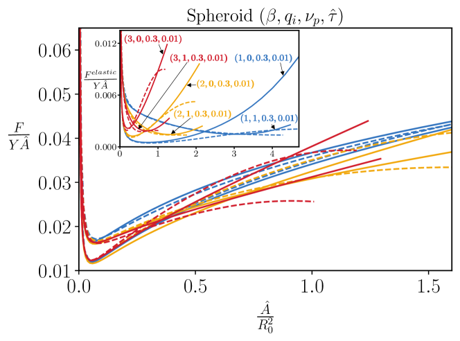
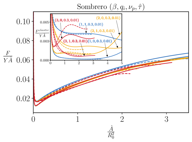
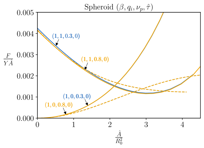
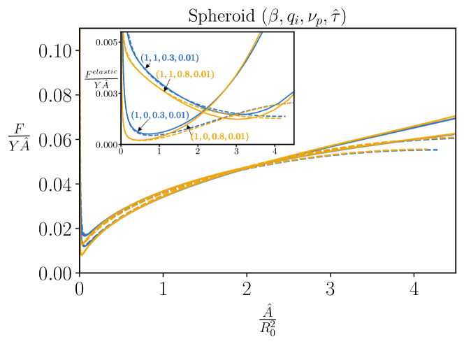
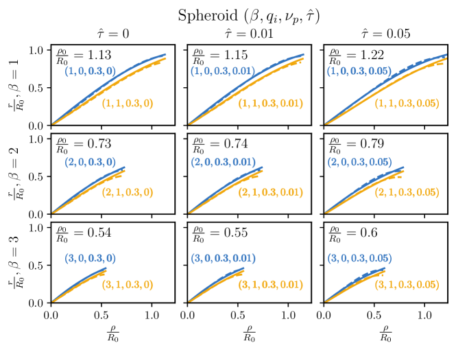
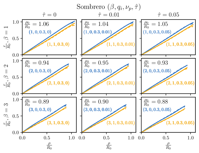
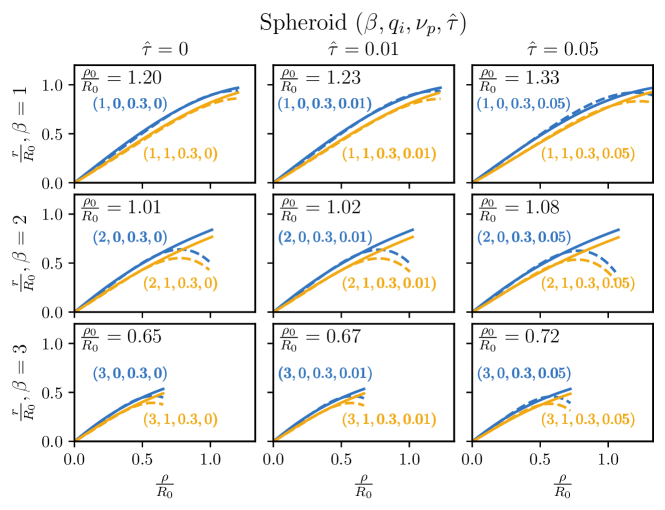
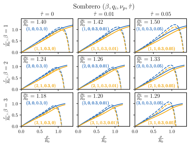
V Additional Plots
References
- Seung and Nelson [1988] H. S. Seung and D. R. Nelson, Defects in flexible membranes with crystalline order, Physical Review A 38, 1005 (1988).