Supplementary information: Discovery of stable surfaces with extreme work functions by high-throughput density functional theory and machine learning
Algorithm to Determine Unique Surface Terminations
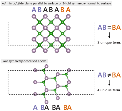
The custom algorithm to determine all unique surface terminations is illustrated in Fig. 1 of the main paper and described in more detail here. First, a list of nearest neighbors (considering only atoms above the reference atom, i.e. with a larger -component, up to a cutoff radius of 10 ) with their distances and chemical elements are compiled for each atom in the slab. Atoms with identical nearest neighbor lists are grouped together into local environment groups (LEGs). In the next step, for each atomic layer (i.e., atoms with the same -component considering a tolerance of 0.1, 0.5, or 1 , depending on which yields the lowest number of unique terminations) the LEG of all atoms in the layer is grouped into a list (one list per layer of atoms). Lastly, the number of unique lists of LEGs determines the number of unique terminations as follows: if the slab is symmetric (i.e., a mirror or glide plane parallel to the surface, or a 2-fold rotation axis normal to the surface), or else. This is due to the fact that the local environments are determined in the positive -direction (only above the reference atom). Hence, a termination A on one side of the slab with termination B underneath might not be equivalent to the A termination on the other side if the slab is not symmetric (as illustrated in Fig. S2).
Previous Version of Work Function Database
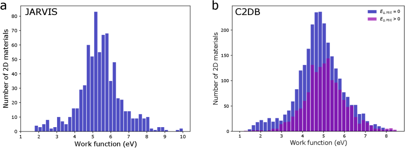
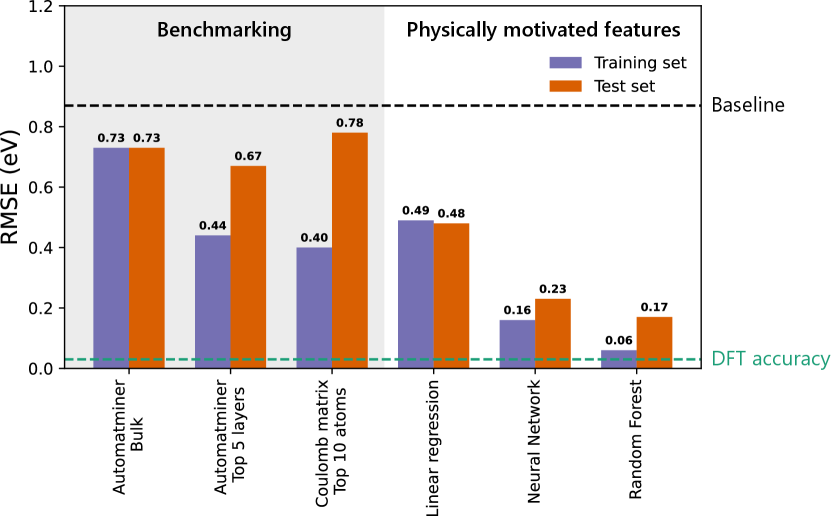
In a previous version of the database we included materials with a non-zero band gap during screening and trained machine learning models on it. However, eventually this database was not utilized in the final paper as band gaps for PBE-level DFT calculations are well-known to be unreliable and hence the work function (positioned at the center of the gap) may also suffer from the same limitation. We do however note that this error is potentially small for materials with a small band gap (less than about half an eV) with a potential partial error cancellation w.r.t. the vacuum energy level. A demonstration of that is the fact that we were able to identify low work function surfaces in non-metallic materials such alkali oxides (e.g., Cs2O2), alkaline vanadates (e.g., BaVO3), and alkali-based anti-fluorite structures (e.g., Rb2O, Rb2S) that were already known in literature (cf. introduction in the main paper). The lowest work function after ionic relaxation was calculated for the (100)-Rb surface of PdRb2C2 at 0.93 eV.
Most high work function candidates in the previous version of the database exhibit a larger bandgap, as expected for flourides, carbides, nitrides and oxides. However, there are a few materials with a zero PBE bangdap in spacegroups 66 (AgO), 139 (CsO2, RbO2, KO2, CaN2), 221 (ReO3), and 225 (PbO2, BiO2). The highest work function after ionic relaxation was calculated for the (110)-F surface of AlF3 at 11.04 eV, likely not in agreement with experimental work functions due to the large band gap error in PBE.
The previous version of the database and the machine learning models trained on that database are available at https://github.com/peterschindler/WorkFunctionDatabase .
| Database | Avg/St.Dev. | Min/Max |
Material IDs
with eV |
Material IDs
with eV |
|---|---|---|---|---|
| JARVIS |
JVASP-8942, JVASP-9002,
JVASP-9059, JVASP-9065, JVASP-19991 |
JVASP-783, JVASP-765,
JVASP-31368, JVASP-31379, JVASP-14441, JVASP-60555, JVASP-14456, JVASP-14458, JVASP-75058, JVASP-75066, JVASP-28011, JVASP-75269, JVASP-28212, JVASP-60599, JVASP-14460, JVASP-60359, JVASP-6244, JVASP-6277, JVASP-27755, JVASP-28153, JVASP-60236, JVASP-75154, JVASP-60593 |
||
| C2DB |
B2H2O2Zr3-b82e8dae99dd,
C2H2O2Nb3-137a187a149c, CH2O2V2-c08bda91646b, C2H2O2Sc3-c6f3a447a0d1, H2N2O2Mn3-46340d3ecfb9, H2O2N3Mn4-0575209d5cde, MnH2O2-3bd136c8a265, OsH2O2-192c92216c12, NCr2H2O2-ff61539f0f78, H2O2C3Cr4-6b206ce0e0a4, H2O2N3Mo4-f9b42b34c5ab, CoH2O2-ebe1b342d92f, CH2O2Y2-310f97f320f8, C2H2O2Ti3-b2d22251cb52, NH2Mn2O2-af38ffeefb90, C2H2O2V3-9c6994bf71a2, H2N2O2Sc3-3c2898c13b0f, H2O2C3Mn4-200df1168731, H2O2C3Mo4-2e0b9178f9f2, FeH2O2-35be111741a4, RhH2O2-44bcea466c91, C2H2O2Y3-cbf305eb62b1, H2O2C3Nb4-760d7905c535, GaH2O2-b42b47e92444, RuH2O2-cd1e59aa5b1c, PdH2Li2-823b99472212, Te2Zn2N4H8-f34362b9488b, H2O2C3Sc4-33474bb0af08, H2O2N3V4-f09ac233cc92, CoCa2O3-40b5f2e2e758, C2H2S2Ti3-4cada7c36f9f, H2N2O2Y3-9030574e723a, H2O2C3Ti4-ec020ed8f687, NiH2O2-4f81e6b4f5aa, CH2Mn2O2-7938aedd38e3, C2H2S2Zr3-2abe5cf3179c, H2O2C3V4-8f5f4356ee52, C2H2O2Cr3-6996d2b04358, H2O2C3W4-4e95b5b75c69, CN-2bae1dfe5219, InH2O2-c58c5def89b7, H2O2C3Y4-82f540c2be44, CH2O2Sc2-f72d84df3799, B2H2O2Ti3-7ef79d62d408, C2H2O2Mn3-aae848e42008, B2H2O2V3-b78d257a108a, C2H2O2Mo3-0cde9e26013d, H2O2N3Cr4-900cb08d8065, CH2O2Ti2-b2d548e0d08a |
Cu2F2-c4860f83a9b8,
GaO2-0a65a6b05ce6, BaTa2O7-877ae50c1f18, SnO2-d5f47e5d4cf7, PbF4-0ace524dc18a, SnF4-a61b85728555, F2Os2-63abc51956be, PbO2-0963dec75c0c, Al2O4-b003ee55f237, BaSb2F12-a8ad6f8ad8ee, F2Ir2-6ab59c2ae465, O4V4F12-05e5d7a8d56c, PdF2-ee10b74aa014, AgSnF6-edbdca5bd78a, AlFeF5-2c9ff5807948, SrTa2O7-a4995476d4ae, C2Ca2F2O6-b46e73deeb64, Ti4O8-92c270a35817, CaAu2F12-73f67052a2e7, F2N2O2Zr3-57adb92deade, RhF2-3574951e1edf |
| sg | Material Family |
Comp. w/
lowest |
Miller planes -
Termination |
mpid (mp-…) | |||
| 8 | KNO2 | (100)-N | 2.30 | 34857 | 2.5 | ||
| KCN | (101)-C+K | 1.21 | 20134 | 5.1 | |||
| 12 | BaNi2As2 | (110)-Ba | 1.91 | 1070400 | 0 | ||
| A2CN2 | A=Na,K | K2CN2 | (001)-K, (\sansmath)-Na | 1.29 | 10408, 541989 | 3.1 | |
| 38 | BaTiO3 | (001)-O-Ba | 1.24 | 5777 | 2.4 | ||
| 44 | NaNO2 | (011)-Na | 1.22 | 2964 | 2.5 | ||
| 63 | AB | A=Sr,Ba, B=Si,Ge,Sn,Pb | BaSi | (110)-A, (010)-A | 1.60 | 20136,872,1730, 2499,2661,2147 | 0 |
| KI | (101)-K | 1.74 | 1078836 | 3.8 | |||
| 71 | AS | A=Rb,Cs | CsS | (101)-A | 1.89 | 29266,558071 | 1.7 |
| A2O2 | A=Rb,Cs | Cs2O2 | (101)-A | 1.12 | 7895,7896 | 1.7-1.8 | |
| AB2D2 | A=Pd,Pt, B=K,Rb, D=O,S,Se,Te | PtRb2S2 | (110)-B, (110)-B+D | 1.62 | 8622,7929,8621,1068813, 7928,540584,8623,1070356, 1070498,1069706,1068941 | 0.7-1.4 | |
| A2B3 | A=Rb,Ba, B=Au,Bi | Rb2Au3 | (101)-A | 1.80 | 569529,11814 | 0 | |
| PtA2B2 | A=Li,Na, B=H,O | PtLi2H2 | (001)-H+Li, (011)-Na | 1.79 | 644136,22313 | 0-1.5 | |
| 107 | ABD3 | A=Sr,Ba,La B=Co,Rh,Ir,Ni,Pt,Au, D=Si,Ge,Sn | BaPtSi3 | (101)-A, (001)-Ba | 1.62 | 1068559,1068048,11879, 30433,13123,1068447,2914, 1070137,1069809,20910, 1067925,22346,1070124, 1069139,1070247,1069708 | 0 |
| 123 | LiPdH | (100)-H-Li | 2.19 | 1018133 | 0 | ||
| CaFeO2 | (100)-Ca-O | 2.31 | 19842 | 0 | |||
| 139 | AB2 | A=Rb,Ca,Sr B=N,O | SrN2 | (101)-A, (111)-N, (110)-A+B | 1.61 | 12105,10564,2697, 1009657 | 0-2.9 |
| AB2D2 | A=Cs,Ba,La,Rh, B=Mg,Co,Rh,Ni,Pd,Pt,Cu,Ag,Zn,Al, D=Si,Ge,Sn,P,As,Sb,S,Se | CsCo2Se2 | (101)-A, (101)-Li+N, (001)-Ba | 1.67 | 9473,31059,8583,21057, 560663,1070267,7882, 6963,7875,12863,9247, 9610,571343,6962 | 0-3.8 | |
| AB2D2 | A=Zn,Pd,Bi, B=Ca,Ba,Sr,Li,Na,La, D=N,H,O | ZnBa2N2 | (001)-B+D, (101)-Sr, (101)-O | 1.42 | 8818,9307,9306, 644389,23954,1070601 | 0-0.9 | |
| AB4 | A=Rb,Ba, B=Al,Ga,In | BaAl4 | (001)-Rb, (101)-Ba | 1.96 | 21477,22687,1903,335 | 0 | |
| 160 | AIO3 | A=K,Rb | RbIO3 | (101)-A+O, (001)-I | 1.35 | 27193,552729 | 3.0-3.2 |
| 164 | BaSi2 | (100)-Ba | 1.77 | 7655 | 0 | ||
| AB2C2 | A=Pd,Pt, B=K,Rb,Cs | PdRb2C2 | (100)-B, (001)-B | 0.93 | 976876,505825,505824, 10918 | 1.7-2.1 | |
| AB2D2 | A=Mg,Zr,Mn, B=Li,Be, D=N,O | ZrLi2N2 | (001)-B | 1.82 | 19279,3216,11917 | 1.6-4.1 | |
| 166 | ABD2 | A=K,Rb,Cs, B=Bi,Y,La,Pr,Sm,Gd,Tb,Ho,Er,Lu,Cr,Tl, D=O,S,Se,Te | RbBiS2 | (101)-A, (101)-A+D | 1.41 | 30041,8175,16763,9085, 11739,561586,4026, 9362,10780,10782, 9364,9367,10783, 7045,561619,9082 | 0.1-2.6 |
| 186 | LiI | (101)-Li, (001)-I | 1.42 | 570935 | 4.4 | ||
| 187 | BaAB | A=Ge,As,Sb, B=Pd,Pt,Al | BaSbPt | (100)-Ba | 1.81 | 8606,13272,9744 | 0 |
| 191 | BaSi2 | (111)-Ba | 1.89 | 7701 | 0 | ||
| 194 | AB | A=Li,Ba, B=Pd,Pt,B | BaPt | (100)-A | 1.72 | 1064367,31498,1001835 | 0 |
| 221 | AB | A=Rb,Cs,Cl, B=Au,Tl,Br | RbAu | (111)-A | 1.42 | 2667,30373,22906,23167 | 0.7-4.8 |
| ABD3 | A=K,Rb,Cs,Sr,Ba, B=Mg,Ca,Zr,Hf,V,Cr,Mn,Sn, D=H,O,F,Cl,Br | BaVO3 | (110)-B+D, (100)-A+D | 1.16 | 27214,1070375,600089, 23949,644203,3323, 558749,23737,3834, 1017465,20029,4551 | 0-3.8 | |
| 225 | AB | A=Li,K,Rb,La,Pr, B=H,S,Se,Cl | KH | (110)-A+B, (100)-A+B, (100)-B | 1.76 | 24721,2350,24084,2495, 23703,1161,22905 | 0-6.4 |
| A2B | A=Li,Na,K,Rb, B=Pd,O,S,Se,Te | Rb2S | (111)-A | 1.19 | 2784,1394,11327,971, 2352,1022,8041,2530, 8426,1266,1747,648, 1960,2286,1062711 | 1.1-5.0 | |
| AH2 | A=La,Pr | LaH2 | (110)-A+H | 1.80 | 24153,24095 | 0 | |
| AH3 | A=La,Ce | LaH3 | (110)-H | 2.07 | 1018144,1008376 | 0 | |
| sg | Material Family |
Comp. w/
highest |
Miller planes -
Termination |
mpid (mp-…) | |||
| 8 | KCN | (110)-C, (001)-C | 8.36 | 20134 | 5.1 | ||
| 12 | LiCuO2 | (\sansmath)-O | 8.16 | 9158 | 0.4 | ||
| Na2CN2 | (001)-N | 8.96 | 541989 | 3 | |||
| 38 | ABO3 | A=K,Ba,Zr, B=Ti,Nb,Pb | ZrPbO3 | (010)-O, (110)-O | 9.44 | 20337,5777,5246 | 2.1-3.3 |
| 39 | TlF | (010)-F | 9.11 | 558134 | 3 | ||
| 44 | NaO3 | (010)-O, (001)-O | 8.80 | 22464 | 0.6 | ||
| 63 | TlCl | (010)-Cl | 8.07 | 571079 | 2.7 | ||
| 66 | AgO | (001)-O | 8.11 | 499 | 0 | ||
| 99 | KNbO3 | (001)-O | 9.47 | 4342 | 1.6 | ||
| 139 | AB2 | A=K,Rb,Cs,Ca,Sr, B=N,O | CaO2 | (001)-B | 9.68 | 1441,12105,1866, 1009657,634859,2697 | 0-2.9 |
| Bi2SeO2 | (101)-O | 8.34 | 552098 | 0.4 | |||
| AF4 | A=Sn,Pb | SnF4 | (100)-F, (101)-F, (110)-F | 10.77 | 341,2706 | 2.0-3.2 | |
| 155 | ScF3 | (110)-F | 8.15 | 559092 | 6.1 | ||
| 160 | ATlO3 | A=Br,I | ITlO3 | (101)-O | 8.81 | 29798,22981 | 3.1-3.7 |
| ABO3 | A=K,Rb, B=Br,I | RbIO3 | (001)-O, (101)-O | 8.81 | 22958,27193,552729 | 3.0-4.1 | |
| BaCO3 | (101)-O | 8.71 | 4559 | 4.4 | |||
| BaTiO3 | (101)-O, (001)-O | 9.45 | 5020 | 2.6 | |||
| 164 | A2BD2 | A=Mg,La, B=Br,S,Se, D=N,O | La2SO2 | (001)-D | 9.18 | 11917,7233,4511 | 3.1-4.1 |
| A2O3 | A=La,Bi | Bi2O3 | (001)-O | 9.25 | 1017552,1968 | 1.4-3.9 | |
| 166 | ABD2 | A=Na,K,Rb,Sr, B=Sc,Y,La,Zr,Nb,Ta,Mo,Rh,Hg,Al,Tl, D=N,O | NaScO2 | (001)-D | 9.62 | 9382,5475,3056,8188, 7958,7017,7748,8145, 7914,8409,978857, 8830,578610 | 0.3-4.8 |
| 186 | AB | A=Mg,Al,Ga,In,Si, B=C,N,O | AlN | (001)-B, (101)-B | 9.23 | 22205,7140,804,549706,661 | 0.5-4.1 |
| 216 | AB | A=Zn,Si, B=C,O | ZnO | (111)-B | 9.80 | 8062,1986 | 0.6-1.6 |
| 221 | ABF3 | A=K,Rb,Cs,Ba, B=Li,Mg,Ca,Cd | BaLiF3 | (110)-F, (110)-B+F | 9.05 | 8399,7104,3654,6951, 8402,3448,10175,4950, 8401,10250 | 3.6-7.2 |
| CsCdCl3 | (110)-Cl | 8.02 | 568544 | 1.9 | |||
| AB3 | A=Sc,W,Re,Al, B=O,F | AlF3 | (111)-B, (110)-B, (100)-O | 11.04 | 19390,190,10694,8039 | 0-7.7 | |
| CsCl | (100)-Cl | 8.13 | 22865 | 5.5 | |||
| 225 | AB | A=Li,Na,K,Rb,Cs,Ca,Cd, B=O,F,Cl | NaF | (111)-B | 10.40 | 23295,573697,1784,2605, 1132,22905,682,463 | 0-6.4 |
| AB2 | A=Sr,Ba,Cd,Hg,Pb,Bi, B=O,F,Cl | CdF2 | (111)-B, (100)-B | 10.80 | 568662,23209,20158,315, 32548,241,8177 | 0-5.6 | |