Supervised Contrastive Prototype Learning:
Augmentation Free Robust Neural Network
Abstract
Transformations in the input space of Deep Neural Networks (DNN) lead to unintended changes in the feature space. Almost perceptually identical inputs, such as adversarial examples, can have significantly distant feature representations. On the contrary, Out-of-Distribution (OOD) samples can have highly similar feature representations to training set samples. Our theoretical analysis for DNNs trained with a categorical classification head suggests that the inflexible logit space restricted by the classification problem size is one of the root causes for the lack of robustness. Our second observation is that DNNs over-fit to the training augmentation technique and do not learn nuance invariant representations. Inspired by the recent success of prototypical and contrastive learning frameworks for both improving robustness and learning nuance invariant representations, we propose a training framework, Supervised Contrastive Prototype Learning (SCPL). We use N-pair contrastive loss with prototypes of the same and opposite classes and replace a categorical classification head with a Prototype Classification Head (PCH). Our approach is sample efficient, does not require sample mining, can be implemented on any existing DNN without modification to their architecture, and combined with other training augmentation techniques. We empirically evaluate the clean robustness of our method on out-of-distribution and adversarial samples. Our framework outperforms other state-of-the-art contrastive and prototype learning approaches in robustness.


1 Introduction
DNNs are known for their poor performance in generalizing to unseen inputs or simple image transformations, such as rotation (Nguyen, Yosinski, and Clune 2015; Guo et al. 2017). Two inputs with insignificant distance in the input space can produce significantly distant feature representations that lead to misclassification. On the contrary, input that is perceptually different from the training samples, such as random noise, can result in feature representations nearly identical to the training samples. In this work, we use the term robustness to refer to the property of DNN to learn an equidistant projection from the input space to the feature space. We identify two main failure cases in DNN; lack of robustness against perturbations, and against nuances.

Robustness against perturbations can be evaluated with an input crafted by an adversarial attack, where an insignificant perturbation on the input space can cause a significant perturbation on the feature space (Szegedy et al. 2013). Similarly, robustness against nuances can be observed with the weakness of DNN where they assign nearly identical feature representations to input that is significantly distant in the input space, such as between random noise and training samples.

Previous work improves the robustness of DNNs with training augmentation techniques specific to the problem they solve. For example, some work (Papernot et al. 2016; Madry et al. 2017; Papernot et al. 2017) improves adversarial robustness by including adversarial-generated samples in the training set. OOD detection methods use samples from the OOD set (Lee et al. 2017; Liang, Li, and Srikant 2017) or an auxiliary dataset (Hendrycks, Mazeika, and Dietterich 2018) during training.
Previous work in contrastive learning (Chen et al. 2020b) identifies training augmentation techniques as one of the primary contributing factors to learning robust feature representations invariant to nuances in the input. In this work, we also view that training augmentation techniques are necessary for learning representations invariant to noise. However, we identify two issues with current approaches in training augmentation.
First, DNNs are prone to over-fitting. We find that, for multiple architectures, the majority of OOD samples are assigned to the most difficult class, the one with the least salient features. Our observation is at odds with the goal of a classifier to learn salient features for every class. For example, for a pretrained ResNet classifier, 99% of uniform random noise is assigned to class 104 with high probability (Appendix fig. S2 c). This suggests a failure of learning, whereby all kinds of unknown images are assigned to the most uncertain class (here, 104). Additionally, DNNs over-fit the augmentation technique used to train the classifier. Previous work (He et al. 2016; Simonyan and Zisserman 2014) resize training images to 256 pixels on the shortest side and then randomly crop them to (224x224) pixels when training on ImageNet. fig. 5 visualizes artifacts of over-fitting to the augmentation technique used during training. The model is biased to the least salient features when predicting out-of-distribution images.
Secondly, data augmentation techniques are expensive, especially for OOD methods that require samples from an out-of-distribution set or an auxiliary dataset. Such methods can be limited in practical settings where additional data is scarce. Similarly, generating adversarial examples for every training iteration is expensive and the current state-of-the-art (Wong, Rice, and Kolter 2020) focuses on improving computational performance. Current training augmentation solutions are a quick fix to a systematic problem, where the issue of robustness is an issue of generalization (Xu and Mannor 2012).
Contrastive Learning (Hadsell, Chopra, and LeCun 2006) approaches do not directly solve for a task but optimize a similarity metric such as the euclidean distance or cosine similarity between feature vectors. Previous contrastive learning work has been successful on downstream tasks such as classification, zero-shot learning, and more (Wang et al. 2018; Xu et al. 2020; Wang et al. 2017; Chen et al. 2017). Additionally, the metric space learned by such models can be robust to both adversarial examples and OOD. The focus of state-of-the-art contrastive learning approaches (Chen et al. 2020a; Khosla et al. 2020) has been to find effective ways to sample pairs that are of the same class (“positive pair”) and one of the most-similar other classes (“negative pair”) that produce meaningful gradients. The sample mining process is computationally expensive and the downstream task performance is sensitive to both the sampling method and the sample size (Kaya and Bilge 2019)
Prototypical Learning (PL) uses a set of vectors (prototypes) to represent a class and is an extension of k-means, where each of the K vectors is a prototype. PL has been used in combination with different learning paradigms such as pattern recognition (Liu and Nakagawa 2001) and more recently has been used both for zero-shot and few-shot learning due to the generalization and sample efficiency (Snell, Swersky, and Zemel 2017). Frameworks have been proposed that implement PL in both supervised and unsupervised settings (Yang et al. 2018a; Li et al. 2020).
Our goal is to design a model that does not depend on any training augmentation technique or auxiliary datasets to achieve high robustness. Motivated by the recent success of Contrastive Learning and Prototypical Learning approaches, in this work we propose the Prototype Classification Head (PCH). Our proposed method combines a classification task with a purely contrastive, sample efficient loss, and can be trained end-to-end with a DNN backbone. PCH is used at the penultimate feature representation of a DNN and replaces the classification head. We use a set of prototype vectors to represent a cluster of feature vectors of the same class. We further improve on previous prototype learning approaches and use N-Prototype Loss which increases inter-class separability and intra-class compactness among training samples. Our approach creates more robust models without additional tricks. Our contribution in detail:
-
•
To the best of our knowledge, this is the first work to combine prototype learning with a purely contrastive loss between prototypes and samples, N-Prototype Loss
-
•
Compared to traditional prototype and contrastive learning methods, our framework uses prototypes to represent a class and does not require intra-batch sample mining.
-
•
Our proposed framework is flexible and can be added to any existing DNN architectures without any further modifications.
-
•
We provide a theoretical justification for the improved robustness, and conduct quantitative experiments that outperform other state-of-art methods
2 Related Work
We identify Prototype Learning approaches and Contrastive Learning approaches as two closely related categories of work that improve the robustness of DNN classifiers.
Triplet loss (Hermans, Beyer, and Leibe 2017) uses one negative and positive pair for each sample to learn a metric and can be sensitive to noise which leads to over-fitting. N-pair(Sohn 2016a) loss decreases the similarity between multiple negative pairs and increases the similarity between a positive pair. Current contrastive learning approaches suffer from poor quality sample pairs that generate uninformative sub-gradients which lead to poor model convergence. Mining for informative pairs such as hard negatives can be computationally expensive. Several approaches have been proposed to improve on the sample mining problem. (Duan et al. 2018) train a separate negative sample generator jointly with a DNN that augments “easy” negative samples with “hard” negative samples. Lifted Structured Loss (LSL) (Oh Song et al. 2016) uses multiple positive and negative pairs in the importance sampling method to improve sample mining of hard negative pairs. However, sample mining techniques are computationally expensive. In contrast, we use learned prototypes for positive and negative pairs and thus avoid the sample mining problem.
Contrastive learning losses are applied in a supervised setting. (Mao et al. 2019) use Triplet loss in an adversarial training setting as an auxilary training objective to the cross-entropy loss. Several contrastive learning framework such as SimCLR (Chen et al. 2020b), MoCo (He et al. 2020) and BYOL (Grill et al. 2020) use a generalized version of N-pair loss (InfoNCE) on the feature representation of an augmented sample to create a positive pair and treat all other samples in a batch as negative. Work by (Li et al. 2020) add an additional loss term to the NCE loss that compares the original sample with prototypes of the same cluster and r negative prototypes. Both the positive and negative prototypes are determined using an expectation maximization clustering framework at every training iteration. In contrast, we assign prototypes to each corresponding class in a supervised setting. Additionally, we use a single training objective between each sample and multiple prototypes, and have a flexible penultimate feature dimension which we identify to be the root cause of the improved robustness. Lastly, our method is orthogonal to other unsupervised contrastive learning approaches and any training augmentation techniques or specific backbone architectures (Chen et al. 2020b; He et al. 2020; Grill et al. 2020) can be extended to our framework.
(Mustafa et al. 2019) apply Prototype Conformity Loss (PCL) as the cross-entropy of the cosine similarity between the feature representation of a sample and the true class prototype vector. For every intermediate representation, an auxiliary network is trained to enforce the intra-class compactness and inter-class separation using the learned prototypes. In contrast to our method, it requires modifying the existing network architecture and can not be directly applied to any existing architecture. Additional work (Mettes, van der Pol, and Snoek 2019; Chen et al. 2021) define fixed prototypes based on an inductive bias for the latent space geometry and maximize the cosine similarity between a sample and the positive class prototype. In contrast to our method, the loss function is applied between multiple sample feature representations and with multiple prototypes from the positive and negative class. Lastly, in our framework the prototypes are learned end-to-end with the DNN. Maintaining fixed prototypes is orthogonal to our method and can be considered as a special case of our framework.
The work that is most similar to ours is (Yang et al. 2018b) that use Distance-based Cross-Entropy (DCE) loss and (Liu et al. 2020) that extend on DCE with an additional loss term Prototype Encoding Cost (PEC). DCE is applied between the closest positive class prototype and a sample, while PEC is the norm between the positive class prototype and the penultimate feature representation. DCE and PEC are optimized jointly for both the network parameters and learned prototypes. Similarly, our framework is applied to the penultimate feature representation. Contrary to DCE and PEC, at every step our method increases the distance between a sample and multiple () opposite class prototypes and reduces the distance to the closest positive prototype.
There are additional work (Yang et al. 2020; Shu et al. 2020) that use prototype learning for a specific problem but can be seen as derivation of more general frameworks. In this work and for reasons of clarity we provide a generalized definition of the state-of-the-art approaches in section 3. Extensive experiments show that our method outperforms other state-of-the-art (Mao et al. 2019; Chen et al. 2020b; Yang et al. 2018a) methods in clean robustness and does not require training augmentation techniques to achieve high robustness. Finally, when compared to other metric learning approaches, our approach does not require sample mining.
3 Preliminary
In this work, we consider the issue of robustness from two angles. Robustness against data samples crafted by an adversary and robustness against samples that are out-of-distribution compared to the training data set.
Out-of-Distribution Robustness (OOD) evaluates a classifier trained on a dataset with an auxiliary function on a test dataset with such that
| (1) |
In this work, we do not design a specific method to our model for OOD detection and use work by (Hendrycks and Gimpel 2018).
OOD Baseline (Hendrycks and Gimpel 2018) normalize the predicted class similarity for a sample and classifier and use the maximum value of the prediction scores for all classes as the confidence score
| (2) |
where a confidence threshold is used to determine if . The robustness of a classifier is then determined by the performance of in correctly classifying in and out-of-distribution samples for a fixed .
Adversarial Robustness measures the accuracy of a DNN with in correctly predicting a clean sample , after a perturbation has been applied by an adversary, with perturbation budget such that
| (3) |
where denotes the loss function used to train and is the p-norm of with . As such, the adversarial example lies within an -ball centered at .
A robust model can correctly classify a perturbed sample that is within the perturbation budget. In this work, we consider adversaries that can manipulate a data sample in and space.
We consider the following adversarial attack settings: Fast Gradient Sign Method (FGSM) (Goodfellow, Shlens, and Szegedy 2014),
Basic Iterative Method (BIM) (Kurakin, Goodfellow, and Bengio 2016)
, Projected Gradient Descent (PGD) (Madry et al. 2017) and AutoAttack (Croce and Hein 2020).
Prototype Distance based Cross Entropy (DCE)
Prototypical frameworks (Yang et al. 2018b; Liu et al. 2020) minimize the distance between prototypes for a task with K classes and sample feature vectors . A similarity matrix between a given feature vector and all prototypes is normalized to satisfy the non-negative and sum-to-one properties of probabilities such that
| (4) |
where y is the true class of sample and is a hyper-parameter. Objective eq. 4 is a generalization of the traditional categorical cross-entropy, when the cosine similarity is used as a similarity function and the prototypes are fixed one-hot vectors.
Auxilary Contrastive Loss
There are work (Mao et al. 2019) that use a contrastive loss that is auxilary to the primary categorical cross-entropy classification loss.
Auxilary Triplet Loss () (Chen et al. 2017) denoted by can be used for classification tasks when optimized jointly with a cross-entropy loss and is computed by eq. 5
| (5) |
with and where is a feature representation of , and and are the feature representations of a positive and negative sample to respectively. is a positive coefficient that provides a trade-off between and , and is the weight for the feature norm. The formulation of the ATL in this section is a generalization of (Mao et al. 2019) but without the use of adversarially augmented samples.
Auxilary N-pair Loss (ANL), We extend ATL by replacing with an InfoNCE Loss Objective (Sohn 2016b) in eq. 5 where is calculated on a (N+1)-tuple , and is the set of feature representations from negative samples to . denotes the total loss calculated by eq. 6
| (6) |
where is the similarity function and all samples are mined identical to ATL. ANL is an interpretation of SimCLR, MoCo and BYOL but applied in a supervised setting and without any training augmentation techniques.
4 Method
Supervised Constrastive Prototype Learning (SCPL) uses a DNN as feature extractor, where is the raw input, the parameters of the model and the learned feature representation of . We apply a Prototype Classification Head on the hidden feature representation of .
The Prototype Classification Head (PCH) is composed of multiple learnable prototype vectors where is the index from the set of classes , is the index from the set of prototypes for class and is the total number of prototypes of the same class. For our experiments, we use the same number of prototypes for all classes, but this assumption can be relaxed for future works.
Inference
We classify a sample by prototype-matching. Given input we compare the extracted representation with all prototypes and assign it to the class with index of the closest prototype based on a metric sim such that
| (7) |
Learning
The trainable parameters in our framework are the parameters for the DNN and the prototypes for each class which are optimized jointly in an end-to-end manner with a single loss function such that
| (8) |
where is the N-Prototype Loss, the Prototype Norm and is a hyper-parameter that controls the weight of the prototype norm. The proposed framework can be extended to other metric learning loss functions such as Contrastive, Triplet, and N-pair. Instead of calculating a metric between samples, we calculate the same metric between prototype vectors and the feature representation of samples. For our experiments, we use N-Prototype Loss.
N-Prototype Loss is computed between the feature representation of the training sample with label and the closest prototype vector from the positive class over the set of the closest prototypes from all negative classes where denotes the total loss calculated by eq. 9
| (9) |
Prototype Norm further improves the compactness of learned prototypes by adding a regularization term to the objective loss function such that
| (10) |
The prototype norm serves the same purpose as an -norm regularization objective to reduce the complexity of the solution space for a sim metric. Thus, improves intra-class compactness and inter-class separability by pulling a feature vector closer to the true class prototype. A difference between eq. 6 and eq. 9 is in the use of prototypes as opposed to negative and positive sample pairs and is highlighted in fig. 2.
Provably Robust Framework
A categorical classifier learns a decision boundary on a feature space that has the same dimensionality as the size of the classification task. For example, a four-way classification task would produce a four-dimensional feature space, for which each dimension is a feature that represents the probability that a sample belongs to each respective class. We identify the cause of the robustness-accuracy trade-off (Tsipras et al. 2018) to be the direct relationship between the feature space dimensionality restricted by the number of classes (“problem size”). An illustration on the difference between categorical classification head and PCH is highlighted in fig. 3.
PCH has a flexible independent of the problem size dimensionality. This allows us to show that the improved performance is a consequence of the flexible dimensionality of the learned feature representation for our method and provide a detailed proof in the Appendix sec. A.
Our experiments corroborate the theoretical implications. We can increase the robustness of the model by increasing and models robust to Gaussian noise are also robust to adversarial attacks. For reasons of brevity we provide additional analysis and experiments that validate our theoretical findings in the Appendix sec. B.
5 Experiments
| Clean | FGSM | PGD | BIM | ||||
|---|---|---|---|---|---|---|---|
| MNIST | LeNet | 99.39 | 11.9 | 1.66 | 76.98 | 26.31 | 99.01 |
| DCE | 99.02 | 11.75 | 0.72 | 73.12 | 25.70 | 98.43 | |
| ATL | 99.32 | 42.13 | 9.75 | 75.54 | 33.69 | 98.85 | |
| ANL | 99.42 | 48.13 | 4.42 | 76.99 | 49.09 | 99.06 | |
| Ours | 99.45 | 65.65 | 27.65 | 90.02 | 79.03 | 99.23 | |
| CIFAR | ResNet | 82.76 | 10.83 | 0.10 | 0.14 | 0.48 | 56.93 |
| DCE | 82.28 | 26.37 | 6.37 | 8.81 | 10.07 | 55.83 | |
| ATL | 83.45 | 16.4 | 0.39 | 0.72 | 1.96 | 57.94 | |
| ANL | 83.89 | 13.85 | 3.59 | 4.23 | 6.26 | 56.24 | |
| Ours | 88.980 | 56.8 | 31.56 | 31.23 | 44.86 | 71.47 | |
| SVHN | ResNet | 92.13 | 16.95 | 0.14 | 0.14 | 0.71 | 63.56 |
| DCE | 92.17 | 50.99 | 5.64 | 8.23 | 17.39 | 72.25 | |
| ATL | 92.78 | 18.85 | 1.10 | 1.41 | 3.41 | 72.08 | |
| ANL | 92.85 | 34.14 | 23.18 | 23.60 | 23.82 | 70.34 | |
| Ours | 94.9 | 81.06 | 56.10 | 58.02 | 71.90 | 88.08 |
Datasets and Models
We extensively evaluate the proposed method on three datasets, MNIST (LeCun, Cortes, and Burges 2010), CIFAR10 (Krizhevsky 2009), and Street-View House Numbers(SVHN) (Netzer et al. 2011). We use Ray (Liaw et al. 2018) optimization framework on a GPU cluster. We provide larger figures and additional experiments in the supplementary material.
We use the categorical cross-entropy loss function for all baselines. As a backbone we use ResNet-18 (He et al. 2016) for CIFAR10 and SVHN datasets and LeNet (LeCun et al. 1989) for MNIST.
For baselines, we consider metric learning and convolutional prototype learning approaches as described in section 3. We compare our method with Auxilary Triplet Loss “ATL” from section 3 used by (Mao et al. 2019). We also compare with Auxilary N-pair Loss “ANL” from section 3 where we use one negative pair per class in which is the interpertation of SimCLR, BYOL and MoCo for a supervised-learning setting. Finally we compare with generalized convolutional prototype learning (GCPL) framework (Yang et al. 2018a; Liu et al. 2020) and denote it as “DCE”.
and use a dimension of 64, and a of 0.1 for .
Results
Clean Robustness
|
|
|
|
|
||||||||||||||||
|---|---|---|---|---|---|---|---|---|---|---|---|---|---|---|---|---|---|---|---|---|
| ImageNet | ResNet | 86.8% | 31.4% | 73.8% | 72.9% | 68.1% | ||||||||||||||
| DCE | 89.2% | 16.7% | 86.4% | 90.4% | 75.9% | |||||||||||||||
| ATL | 42.5% | 11.4% | 93.9% | 95.4% | 91.5% | |||||||||||||||
| ANL | 62.7% | 19.3% | 86.4% | 84.0% | 82.6% | |||||||||||||||
| Ours | 9.9% | 5.3% | 96.3% | 97.7% | 91.7% | |||||||||||||||
| LSUN | ResNet | 68.5% | 20.1% | 86.4% | 87.2% | 82.3% | ||||||||||||||
| DCE | 94.0% | 21.5% | 80.6% | 83.4% | 70.2% | |||||||||||||||
| ATL | 57.3% | 15.2% | 90.8% | 92.6% | 87.5% | |||||||||||||||
| ANL | 53.2% | 18.0% | 87.1% | 82.2% | 85.0% | |||||||||||||||
| Ours | 9.2% | 5.6% | 96.8% | 97.8% | 94.6% | |||||||||||||||
| Gaussian noise | ResNet | 92.5% | 44.3% | 57.8% | 49.5% | 53.1% | ||||||||||||||
| DCE | 23.0% | 7.6% | 96.3% | 97.4% | 93.7% | |||||||||||||||
| ATL | 36.9% | 10.8% | 94.7% | 95.8% | 92.7% | |||||||||||||||
| ANL | 97.3% | 50.0% | 41.0% | 41.7% | 45.0% | |||||||||||||||
| Ours | 4.8% | 2.8% | 95.5% | 97.7% | 86.2% |


We evaluate the “Clean” accuracy on the unperturbed test set and the accuracy on the same test set after it has been perturbed by FGSM, PGD, BIM, PGD with random start in space “”, PGD in space “” and AutoAttack. For all baselines we evaluate the robustness of multiple checkpoints and report the numbers from the best performing checkpoint.
The results in table 1 demonstrate that our method outperforms other baselines for all five types of attacks with a larger improvement on stronger attack settings (PGD, BIM, ) and more complex datasets such as for CIFAR and SVHN. The improved robustness is larger for stronger attacks in . Furthermore, when evaluated in AutoAttack, our model is the only that can achieve 0.1109 robustness, as compared to 0.0 for all other baselines.
In agreement with previous work (Tsipras et al. 2018) we observe a trade-off between clean accuracy and robustness. All model can reach a clean accuracy comparable to previously reported benchmarks (He et al. 2016) but at the cost of robustness. When evaluating a model at the check-point of peak robustness the clean accuracy significantly suffers for non-robust model. Where the clean accuracy drops from 92.2% to 82.76% for a ResNet backbone.
Out-of-Distribution (OOD)
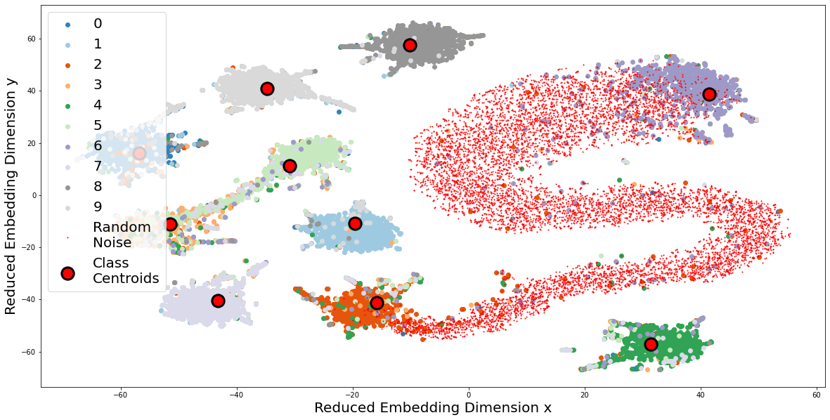
We train all baselines and our own model on SVHN as and calculate the ability to detect out-of-distribution datasets such as ImageNet (Le and Yang 2015), LSUN (Yu et al. 2015) and Gaussian Noise using methodology from (Hendrycks, Mazeika, and Dietterich 2018) and metrics from (Liang, Li, and Srikant 2017). We use a normal distribution for Gaussian Noise, normalize and clip the values to be within the same range as SVHN. Results are presented in table 2. Based on Detection Error, our method surpasses the second-best approaches by 6.1% for ImageNet, 44% for LSUN, and 4.8% for Gaussian noise out-of-distribution datasets. We perform dimensionality reduction (t-SNE) (Van der Maaten and Hinton 2008) on the feature representation and visualize the inter-class separability to Gaussian noise outliers in supplementary fig. 2
and attach a larger size figure in our supplementary. From the figure it can be observed that most outliers are outside the classification boundary of the prototype.
Attack Detection To further demonstrate the robustness of our framework, we test our model and baselines with the same methodology as in the OOD detection experiment. We use PGD to generate adversarial samples as . We use CIFAR10 and SVHN as . The experiments evaluate the robustness to detect if a test sample has been perturbed by an adversarial attacker. Results are shown in table 3. Our method significantly outperforms all baselines for every evaluation metric. The detection error for all the baseline methods is 50% with one exception. Since OOD detection is a binary classification task, the results indicate the baselines have no discriminative power in this setting. Our method is the only framework that can detect adversarial samples.
|
|
|
|
|
||||||||||||||||
|---|---|---|---|---|---|---|---|---|---|---|---|---|---|---|---|---|---|---|---|---|
| CIFAR (PGD) | ResNet | 100.0% | 50.0% | 27.9% | 33.5% | 5.1% | ||||||||||||||
| DCE | 97.9% | 50.0% | 22.4% | 34.5% | 32.3% | |||||||||||||||
| ATL | 100.0% | 50.0% | 40.4% | 35.8% | 0.5% | |||||||||||||||
| ANL | 100.0% | 50.0% | 26.7% | 33.2% | 2.8% | |||||||||||||||
| Ours | 89.9% | 37.3% | 66.5% | 67.1% | 62.8% | |||||||||||||||
| SVHN (PGD) | ResNet | 100.0% | 50.0% | 38.5% | 35.3% | 1.8% | ||||||||||||||
| DCE | 89.1% | 41.4% | 50.7% | 45.6% | 55.8% | |||||||||||||||
| ATL | 99.9% | 50.0% | 6.8% | 31.5% | 27.2% | |||||||||||||||
| ANL | 99.7% | 50.0% | 12.0% | 32.4% | 32.2% | |||||||||||||||
| Ours | 76.1% | 38.2% | 66.0% | 68.8% | 65.5% |
Sample efficiency
We evaluate the ability of each model to efficiently learn from training samples. We randomly sample a subset of the SVHN dataset and train multiple models as we vary the sample size. We evaluate and report the best accuracy score and adversarial robustness for an FGSM attack on each model on the entire test set. The increase in accuracy and robustness as the training set ratio increases can be found in fig. 4. Our method is highly robust even with limited training samples. SCPL achieves a 0.87 test accuracy score using only 10 percent of the full training dataset in contrast to 0.6 for a ResNet-18 backbone. We calculate the Return on Investment (ROI) on the training dataset size using the dataset size as cost and adversarial robustness increase as the net gain. SCPL has an ROI of 164% with an increase in robustness from 12.5% to 28.9% and an increase in training samples from 0.1 to 0.2 percent as opposed to the next best model for the same ratio interval, ANL, with an ROI of 33%. The robustness of SCPL increases faster compared to other baselines.
Ablation studies
We perform extensive ablation studies on the hyper-parameters of our method using two datasets, CIFAR10 and SVHN. Results are presented on table 1 and table 2 in the Appendix for CIFAR and SVHN dataset respectively. We train our model with identical training settings for different regularization coefficients and numbers of prototypes per class , with the similarity metrics for train and inference denoted as ( Train / Inference). We denote the base model as ‘base’ which is identical to the Adversarial Robustness experimental set-up with the only difference being that we train for 100 epochs. The results suggest the benefit of is that the features are gathered closer to their intra-class prototypes. We experiment with a cosine similarity which is the Dot-Product (“DP”) loss function for both inference and training. In agreement with our theoretical results, we conclude that “DP” can improve the robustness. In addition, we found that increasing the number of prototypes per class will degrade the model accuracy, which agrees with previous work (Yang et al. 2018a). We hypothesize that too many prototypes can be a difficult optimization objective and the reduced robustness is due to different prototypes providing a larger -Neighbourhood for as we discussed in Provably Robust Framework section 4.
6 Discussion
Our proposed method outperforms the previous state-of-the-art, but there are limitations and potential future improvements. First, the prototypes are initialized with random weights in the current setting, which can lead to poor convergence at the beginning of the training stage. Warm-up methods could further improve model convergence (Arthur and Vassilvitskii 2006).
In addition, the similarity function between feature representations and the decision boundary from theorem Provably Robust Classification in the Appendix can be improved. Related to this is the design of an OOD method specific to our model.
Finally, the inference of our proposed method is based on prototype matching by assigning test examples to the class of their closest prototype, which cannot be directly applied to tasks where a continuous value needs to be predicted (i.e regressional analysis).
7 Conclusion
We propose a supervised contrastive prototype learning (SCPL) framework for learning robust feature representation. We replace the categorical classification layer of a DNN with a Prototype Classification Head (PCH). PCH is an ensemble of prototypes assigned to each class. We train PCH jointly with the DNN using a single optimization objective, N-Prototype Loss. We empirically validate our results and provide a theoretical justification for the improved robustness. We achieve increased robustness without requiring auxiliary data such as adversarial or out-of-distribution examples. Lastly, SCPL requires no modification to the classification backbone and thus is compatible with any existing DNN.
References
- Arthur and Vassilvitskii (2006) Arthur, D.; and Vassilvitskii, S. 2006. k-means++: The advantages of careful seeding. Technical report, Stanford.
- Chen et al. (2021) Chen, G.; Peng, P.; Wang, X.; and Tian, Y. 2021. Adversarial reciprocal points learning for open set recognition. arXiv preprint arXiv:2103.00953.
- Chen et al. (2020a) Chen, T.; Kornblith, S.; Norouzi, M.; and Hinton, G. 2020a. A simple framework for contrastive learning of visual representations. In International conference on machine learning, 1597–1607. PMLR.
- Chen et al. (2020b) Chen, T.; Kornblith, S.; Norouzi, M.; and Hinton, G. E. 2020b. A Simple Framework for Contrastive Learning of Visual Representations. CoRR, abs/2002.05709.
- Chen et al. (2017) Chen, W.; Chen, X.; Zhang, J.; and Huang, K. 2017. Beyond triplet loss: a deep quadruplet network for person re-identification. In Proceedings of the IEEE conference on computer vision and pattern recognition, 403–412.
- Croce and Hein (2020) Croce, F.; and Hein, M. 2020. Reliable evaluation of adversarial robustness with an ensemble of diverse parameter-free attacks. In International conference on machine learning, 2206–2216. PMLR.
- Deng et al. (2009) Deng, J.; Dong, W.; Socher, R.; Li, L.-J.; Li, K.; and Fei-Fei, L. 2009. ImageNet: A Large-Scale Hierarchical Image Database. In CVPR09.
- Duan et al. (2018) Duan, Y.; Zheng, W.; Lin, X.; Lu, J.; and Zhou, J. 2018. Deep adversarial metric learning. In Proceedings of the IEEE Conference on Computer Vision and Pattern Recognition, 2780–2789.
- Goodfellow, Shlens, and Szegedy (2014) Goodfellow, I. J.; Shlens, J.; and Szegedy, C. 2014. Explaining and harnessing adversarial examples. arXiv preprint arXiv:1412.6572.
- Grill et al. (2020) Grill, J.-B.; Strub, F.; Altché, F.; Tallec, C.; Richemond, P.; Buchatskaya, E.; Doersch, C.; Avila Pires, B.; Guo, Z.; Gheshlaghi Azar, M.; et al. 2020. Bootstrap your own latent-a new approach to self-supervised learning. Advances in neural information processing systems, 33: 21271–21284.
- Guo et al. (2017) Guo, C.; Pleiss, G.; Sun, Y.; and Weinberger, K. Q. 2017. On calibration of modern neural networks. In International Conference on Machine Learning, 1321–1330. PMLR.
- Hadsell, Chopra, and LeCun (2006) Hadsell, R.; Chopra, S.; and LeCun, Y. 2006. Dimensionality reduction by learning an invariant mapping. In 2006 IEEE Computer Society Conference on Computer Vision and Pattern Recognition (CVPR’06), volume 2, 1735–1742. IEEE.
- He et al. (2020) He, K.; Fan, H.; Wu, Y.; Xie, S.; and Girshick, R. 2020. Momentum contrast for unsupervised visual representation learning. In Proceedings of the IEEE/CVF conference on computer vision and pattern recognition, 9729–9738.
- He et al. (2016) He, K.; Zhang, X.; Ren, S.; and Sun, J. 2016. Deep residual learning for image recognition. In Proceedings of the IEEE conference on computer vision and pattern recognition, 770–778.
- Hendrycks and Gimpel (2018) Hendrycks, D.; and Gimpel, K. 2018. A Baseline for Detecting Misclassified and Out-of-Distribution Examples in Neural Networks. arXiv:1610.02136.
- Hendrycks, Mazeika, and Dietterich (2018) Hendrycks, D.; Mazeika, M.; and Dietterich, T. 2018. Deep anomaly detection with outlier exposure. arXiv preprint arXiv:1812.04606.
- Hermans, Beyer, and Leibe (2017) Hermans, A.; Beyer, L.; and Leibe, B. 2017. In defense of the triplet loss for person re-identification. arXiv preprint arXiv:1703.07737.
- Kaya and Bilge (2019) Kaya, M.; and Bilge, H. Ş. 2019. Deep metric learning: A survey. Symmetry, 11(9): 1066.
- Khosla et al. (2020) Khosla, P.; Teterwak, P.; Wang, C.; Sarna, A.; Tian, Y.; Isola, P.; Maschinot, A.; Liu, C.; and Krishnan, D. 2020. Supervised contrastive learning. arXiv preprint arXiv:2004.11362.
- Krizhevsky (2009) Krizhevsky, A. 2009. Learning multiple layers of features from tiny images. Technical report.
- Kurakin, Goodfellow, and Bengio (2016) Kurakin, A.; Goodfellow, I.; and Bengio, S. 2016. Adversarial examples in the physical world. arXiv preprint arXiv:1607.02533.
- Le and Yang (2015) Le, Y.; and Yang, X. 2015. Tiny imagenet visual recognition challenge. CS 231N, 7(7): 3.
- LeCun et al. (1989) LeCun, Y.; Boser, B.; Denker, J. S.; Henderson, D.; Howard, R. E.; Hubbard, W.; and Jackel, L. D. 1989. Backpropagation applied to handwritten zip code recognition. Neural computation, 1(4): 541–551.
- LeCun, Cortes, and Burges (2010) LeCun, Y.; Cortes, C.; and Burges, C. 2010. MNIST handwritten digit database. ATT Labs [Online]. Available: http://yann.lecun.com/exdb/mnist, 2.
- Lee et al. (2017) Lee, K.; Lee, H.; Lee, K.; and Shin, J. 2017. Training confidence-calibrated classifiers for detecting out-of-distribution samples. arXiv preprint arXiv:1711.09325.
- Li et al. (2020) Li, J.; Zhou, P.; Xiong, C.; and Hoi, S. C. 2020. Prototypical contrastive learning of unsupervised representations. arXiv preprint arXiv:2005.04966.
- Liang, Li, and Srikant (2017) Liang, S.; Li, Y.; and Srikant, R. 2017. Enhancing the reliability of out-of-distribution image detection in neural networks. arXiv preprint arXiv:1706.02690.
- Liaw et al. (2018) Liaw, R.; Liang, E.; Nishihara, R.; Moritz, P.; Gonzalez, J. E.; and Stoica, I. 2018. Tune: A Research Platform for Distributed Model Selection and Training. arXiv preprint arXiv:1807.05118.
- Liu and Nakagawa (2001) Liu, C.-L.; and Nakagawa, M. 2001. Evaluation of prototype learning algorithms for nearest-neighbor classifier in application to handwritten character recognition. Pattern Recognition, 34(3): 601–615.
- Liu et al. (2020) Liu, Z.; Zhang, X.; Zhu, Z.; Zheng, S.; Zhao, Y.; and Cheng, J. 2020. Convolutional prototype learning for zero-shot recognition. Image and Vision Computing, 98: 103924.
- Madry et al. (2017) Madry, A.; Makelov, A.; Schmidt, L.; Tsipras, D.; and Vladu, A. 2017. Towards deep learning models resistant to adversarial attacks. arXiv preprint arXiv:1706.06083.
- Mao et al. (2019) Mao, C.; Zhong, Z.; Yang, J.; Vondrick, C.; and Ray, B. 2019. Metric Learning for Adversarial Robustness. In Wallach, H.; Larochelle, H.; Beygelzimer, A.; d'Alché-Buc, F.; Fox, E.; and Garnett, R., eds., Advances in Neural Information Processing Systems, volume 32. Curran Associates, Inc.
- Mettes, van der Pol, and Snoek (2019) Mettes, P.; van der Pol, E.; and Snoek, C. 2019. Hyperspherical prototype networks. Advances in neural information processing systems, 32.
- Mustafa et al. (2019) Mustafa, A.; Khan, S.; Hayat, M.; Goecke, R.; Shen, J.; and Shao, L. 2019. Adversarial defense by restricting the hidden space of deep neural networks. In Proceedings of the IEEE International Conference on Computer Vision, 3385–3394.
- Netzer et al. (2011) Netzer, Y.; Wang, T.; Coates, A.; Bissacco, A.; Wu, B.; and Ng, A. Y. 2011. Reading Digits in Natural Images with Unsupervised Feature Learning.
- Nguyen, Yosinski, and Clune (2015) Nguyen, A.; Yosinski, J.; and Clune, J. 2015. Deep neural networks are easily fooled: High confidence predictions for unrecognizable images. In Proceedings of the IEEE conference on computer vision and pattern recognition, 427–436.
- Oh Song et al. (2016) Oh Song, H.; Xiang, Y.; Jegelka, S.; and Savarese, S. 2016. Deep metric learning via lifted structured feature embedding. In Proceedings of the IEEE conference on computer vision and pattern recognition, 4004–4012.
- Papernot et al. (2017) Papernot, N.; McDaniel, P.; Goodfellow, I.; Jha, S.; Celik, Z. B.; and Swami, A. 2017. Practical black-box attacks against machine learning. In Proceedings of the 2017 ACM on Asia conference on computer and communications security, 506–519.
- Papernot et al. (2016) Papernot, N.; McDaniel, P.; Wu, X.; Jha, S.; and Swami, A. 2016. Distillation as a defense to adversarial perturbations against deep neural networks. In 2016 IEEE symposium on security and privacy (SP), 582–597. IEEE.
- Paszke et al. (2019) Paszke, A.; Gross, S.; Massa, F.; Lerer, A.; Bradbury, J.; Chanan, G.; Killeen, T.; Lin, Z.; Gimelshein, N.; Antiga, L.; Desmaison, A.; Kopf, A.; Yang, E.; DeVito, Z.; Raison, M.; Tejani, A.; Chilamkurthy, S.; Steiner, B.; Fang, L.; Bai, J.; and Chintala, S. 2019. PyTorch: An Imperative Style, High-Performance Deep Learning Library. In Wallach, H.; Larochelle, H.; Beygelzimer, A.; d'Alché-Buc, F.; Fox, E.; and Garnett, R., eds., Advances in Neural Information Processing Systems 32, 8024–8035. Curran Associates, Inc.
- Selvaraju et al. (2017) Selvaraju, R. R.; Cogswell, M.; Das, A.; Vedantam, R.; Parikh, D.; and Batra, D. 2017. Grad-cam: Visual explanations from deep networks via gradient-based localization. In Proceedings of the IEEE international conference on computer vision, 618–626.
- Shu et al. (2020) Shu, Y.; Shi, Y.; Wang, Y.; Huang, T.; and Tian, Y. 2020. P-ODN: Prototype-based open deep network for open set recognition. Scientific reports, 10(1): 1–13.
- Simonyan and Zisserman (2014) Simonyan, K.; and Zisserman, A. 2014. Very deep convolutional networks for large-scale image recognition. arXiv preprint arXiv:1409.1556.
- Snell, Swersky, and Zemel (2017) Snell, J.; Swersky, K.; and Zemel, R. S. 2017. Prototypical networks for few-shot learning. arXiv preprint arXiv:1703.05175.
- Sohn (2016a) Sohn, K. 2016a. Improved Deep Metric Learning with Multi-class N-pair Loss Objective. In Lee, D.; Sugiyama, M.; Luxburg, U.; Guyon, I.; and Garnett, R., eds., Advances in Neural Information Processing Systems, volume 29. Curran Associates, Inc.
- Sohn (2016b) Sohn, K. 2016b. Improved deep metric learning with multi-class n-pair loss objective. Advances in neural information processing systems, 29.
- Szegedy et al. (2013) Szegedy, C.; Zaremba, W.; Sutskever, I.; Bruna, J.; Erhan, D.; Goodfellow, I.; and Fergus, R. 2013. Intriguing properties of neural networks. arXiv preprint arXiv:1312.6199.
- Tsipras et al. (2018) Tsipras, D.; Santurkar, S.; Engstrom, L.; Turner, A.; and Madry, A. 2018. Robustness may be at odds with accuracy. arXiv preprint arXiv:1805.12152.
- Van der Maaten and Hinton (2008) Van der Maaten, L.; and Hinton, G. 2008. Visualizing data using t-SNE. Journal of machine learning research, 9(11).
- Wang et al. (2018) Wang, H.; Wang, Y.; Zhou, Z.; Ji, X.; Gong, D.; Zhou, J.; Li, Z.; and Liu, W. 2018. Cosface: Large margin cosine loss for deep face recognition. In Proceedings of the IEEE conference on computer vision and pattern recognition, 5265–5274.
- Wang et al. (2017) Wang, J.; Zhou, F.; Wen, S.; Liu, X.; and Lin, Y. 2017. Deep metric learning with angular loss. In Proceedings of the IEEE International Conference on Computer Vision, 2593–2601.
- Wong, Rice, and Kolter (2020) Wong, E.; Rice, L.; and Kolter, J. Z. 2020. Fast is better than free: Revisiting adversarial training. arXiv preprint arXiv:2001.03994.
- Xu and Mannor (2012) Xu, H.; and Mannor, S. 2012. Robustness and generalization. Machine learning, 86(3): 391–423.
- Xu et al. (2020) Xu, W.; Xian, Y.; Wang, J.; Schiele, B.; and Akata, Z. 2020. Attribute prototype network for zero-shot learning. arXiv preprint arXiv:2008.08290.
- Yang et al. (2018a) Yang, H.-M.; Zhang, X.-Y.; Yin, F.; and Liu, C.-L. 2018a. Robust Classification with Convolutional Prototype Learning. arXiv:1805.03438.
- Yang et al. (2018b) Yang, H.-M.; Zhang, X.-Y.; Yin, F.; and Liu, C.-L. 2018b. Robust classification with convolutional prototype learning. In Proceedings of the IEEE Conference on Computer Vision and Pattern Recognition, 3474–3482.
- Yang et al. (2020) Yang, H.-M.; Zhang, X.-Y.; Yin, F.; Yang, Q.; and Liu, C.-L. 2020. Convolutional prototype network for open set recognition. IEEE Transactions on Pattern Analysis and Machine Intelligence.
- Yu et al. (2015) Yu, F.; Seff, A.; Zhang, Y.; Song, S.; Funkhouser, T.; and Xiao, J. 2015. Lsun: Construction of a large-scale image dataset using deep learning with humans in the loop. arXiv preprint arXiv:1506.03365.
Appendix A Theoretical Results
Provably Robust Framework A categorical classifier learns a decision boundary on a feature space that has the same dimensionality as the size of the classification task. For example, a binary classification task would produce a two-dimensional feature space for which each dimension is a feature that represents the probability that a sample belongs to each respective class. We identify the cause of the robustness-accuracy trade-off (Tsipras et al. 2018) to be the direct relationship between the feature space dimensionality restricted by the number of classes (“problem size”).
For our analysis we define a powerful transformation where is a sample with i.i.d features such that and is the hidden representation. It follows that for any hidden representation of lower dimensionality s.t. a transformation function will be unable to produce a one-to-one mapping between and and thus can not be i.i.d. such that .
Consider a downstream categorical classifier that assign a sample to the class . Assume a strong -norm adversary that can perturb and is bounded by a constant . Perturbations to the input space will lead to perturbations in the hidden representation where for a problem with classes. A non-robust classifier will assign a smaller value for the hidden representation and for the true class of . A robust classifier will be invariant to such noise and will be significantly greater than all other elements of the -set such that .
A categorical classifier has a hidden space dimensionality equivalent to . For any general transformation, as the hidden space dimensionality approaches the input space dimensionality , an optimal transformation can learn and the inter-class distance increases such that . We thus identify that the issue of inter-class separation is due to the restricted hidden representation space for a high dimensional input space.
PCH has a flexible independent of the problem size dimensionality. This allows us to show that the improved performance is a consequence of the flexible dimensionality of the learned feature representation for our method. Theorem 1 can explain the improved robustness as the number of dimensions of the feature space increases. Additionally, we conclude that the similarity metric used is important in creating provably robust classifiers. Although the theorem does not extend to distance, additional conditions on the similarity boundary can be applied using the triangle inequality. In this work, we do not focus on the design of the similarity function or approximation of the decision boundary and consider it an open problem.
A consequence of theorem 1 is that it provides a guarantee of robustness only based on a known classification set . A perturbation that is similar to a sample or a sample that is similar will also be in the -Neighborhood of . Any such perturbation could cause our theoretical framework to become non-robust to . In practice, this would be equivalent to a data-poisoning attack on classifier. Such classifier will be trained to assign class to random noise. Moreover, it would be possible to construct an adversarial example using a perturbation that belongs to any class , since . In practice, is limited by the amount of computational resources but as increases, such perturbation will craft adversarial examples that are perceptually different than the true class or original image. Thus, the strength of our theoretical framework is that any successful adversarial sample would not be perceptually similar to the original input for a classifier trained on natural images and for really large .
Our experiments corroborate the theoretical implications. We can increase the robustness of the model by increasing and models robust to Gaussian noise are also robust to adversarial attacks. We provide detailed proofs in the remainder of this section and additional experiments in appendix B.
Definition 1 (Classification Similarity Function).
compute a metric between two vectors , is distributive over vector addition , is communicative , and is divergent as the number of dimensions increases such that
Definition 2 (Classification Set).
The set is the set of samples for prototype vector where given a positive similarity boundary such that
Theorem 1 (Provably Robust Classification).
Given there exists a similarity boundary and a prototype vector for which there is no perturbation such that the perturbed feature vector is misclassified with but is correctly classified with as the number of feature space dimensions increases with .
Proof: Let be a classification similarity function and let where is in the classification set with the similarity boundary. Let be a perturbation s.t. .
Assume that there exists a s.t. but (1)
By the distributive property we have ,
Let .
There exist an such that , by substitution and thus
By definition is divergent as with and but which is a contradiction.
Appendix B Additional Experiments
The issue of robustness can be viewed as an issue of generalization (Xu and Mannor 2012). We perform additional experiments to corroborate our theoretical findings. We use a VGG-11 (He et al. 2016) model pre-trained on ImageNet as provided by the python library PyTorch (Paszke et al. 2019). We compute the Gradient Activation map (Selvaraju et al. 2017) for all images in three datasets CIFAR-10 (Krizhevsky 2009), ImageNet-1M (Deng et al. 2009), and Gaussian random noise. We compute the mean activation value of all images within each dataset. The mean activation maps at fig. 5 show artifacts of the training settings. He et al. (He et al. 2016) resizes the images during on the shortest side to be 256 pixels during training. The images are then randomly cropped to (224x224). As a consequence, the corners of the original image (32 pixels) will appear less frequently during training. The model learns to ignore the corners as shown by the activation map and over-fit to the center of the image. When random noise is fed such that there are no salient features from which the classifier can correctly assign the class, the network makes predictions based on the image corners. We observe that the salient features the network uses to classify an image are the cropping dimensions. This is an artifact of the classifier overfitting to the augmentation technique used during training.
We analyze the prediction scores for a categorical classification model to find that it makes overconfident predictions for the wrong class. Our method (PCH) assigns high confidence on the in-distribution () dataset CIFAR-10 as can be seen by the area of the red curve in fig. 7(a). Out-of-distribution images are assigned less confident prediction scores for our method.
In contrast, a ResNet-18 model pretrained on ImageNet assigns high confidence predictions to out-of-distribution data. Additionally, the majority of predictions are for a single class. The majority predicted class is the same for a dataset between different runs and random iterations but different between datasets, as can be seen in fig. 7(c).
Lastly, our model (PCH) has high inter-class separation. Out-of-distribution samples are distanced from the class centroids, as can be seen in fig. 6.
| Clean | FGSM | PGD | BIM | |||
| base | 88.980 | 27.370 | 5.240 | 7.340 | 5.870 | 68.090 |
| =0 | 88.630 | 27.500 | 4.120 | 6.230 | 4.170 | 70.720 |
| =0.2 | 88.770 | 28.650 | 6.740 | 10.070 | 6.700 | 73.250 |
| D=2 | 62.420 | 14.200 | 1.020 | 1.030 | 3.000 | 39.360 |
| D=8 | 83.080 | 19.540 | 1.540 | 1.700 | 3.730 | 55.680 |
| C=2 | 88.120 | 29.140 | 6.800 | 9.360 | 6.470 | 67.990 |
| C=5 | 85.810 | 23.660 | 5.040 | 6.870 | 4.560 | 66.310 |
| C=10 | 83.800 | 19.950 | 3.780 | 5.370 | 3.770 | 62.850 |
| / | 83.600 | 23.490 | 5.280 | 7.220 | 5.480 | 64.930 |
| DP/ | 84.100 | 22.730 | 4.500 | 5.030 | 5.320 | 68.450 |
| DP / DP | 82.260 | 19.470 | 3.500 | 4.950 | 3.580 | 63.950 |
| / | 86.340 | 23.940 | 5.600 | 5.760 | 6.230 | 70.060 |
| / | 88.980 | 27.410 | 5.260 | 7.330 | 5.620 | 68.090 |
| / DP | 88.980 | 27.410 | 5.260 | 7.350 | 5.810 | 68.080 |
| Clean | FGSM | PGD | BIM | |||
| base | 94.872 | 52.524 | 8.547 | 17.048 | 10.257 | 85.802 |
| =0 | 94.683 | 50.980 | 6.550 | 15.946 | 9.135 | 86.086 |
| =0.2 | 94.780 | 53.373 | 10.483 | 19.119 | 12.412 | 86.616 |
| D=2 | 79.122 | 42.102 | 6.822 | 8.332 | 8.397 | 62.780 |
| D=8 | 92.617 | 23.660 | 5.040 | 6.870 | 4.560 | 66.310 |
| C=2 | 94.610 | 54.099 | 15.112 | 24.804 | 17.083 | 86.209 |
| C=5 | 94.434 | 48.986 | 8.805 | 17.705 | 10.910 | 85.510 |
| C=10 | 94.073 | 45.164 | 6.457 | 13.299 | 8.313 | 84.342 |
| / | 94.415 | 47.945 | 8.451 | 17.037 | 10.026 | 84.930 |
| DP / | 95.022 | 51.314 | 6.200 | 18.758 | 8.397 | 87.519 |
| DP / DP | 93.654 | 53.619 | 8.831 | 17.920 | 10.191 | 83.171 |
| / | 94.626 | 53.357 | 6.523 | 18.946 | 9.043 | 87.062 |
| / | 94.872 | 52.520 | 8.582 | 17.098 | 10.360 | 85.802 |
| / DP | 94.872 | 52.520 | 8.586 | 17.098 | 10.345 | 85.802 |