Superpoint Gaussian Splatting for Real-Time High-Fidelity Dynamic Scene Reconstruction
Abstract
Rendering novel view images in dynamic scenes is a crucial yet challenging task. Current methods mainly utilize NeRF-based methods to represent the static scene and an additional time-variant MLP to model scene deformations, resulting in relatively low rendering quality as well as slow inference speed. To tackle these challenges, we propose a novel framework named Superpoint Gaussian Splatting (SP-GS). Specifically, our framework first employs explicit 3D Gaussians to reconstruct the scene and then clusters Gaussians with similar properties (e.g., rotation, translation, and location) into superpoints. Empowered by these superpoints, our method manages to extend 3D Gaussian splatting to dynamic scenes with only a slight increase in computational expense. Apart from achieving state-of-the-art visual quality and real-time rendering under high resolutions, the superpoint representation provides a stronger manipulation capability. Extensive experiments demonstrate the practicality and effectiveness of our approach on both synthetic and real-world datasets. Please see our project page at https://dnvtmf.github.io/SP_GS.github.io.
1 Introduction
Synthesizing high-fidelity novel view images of a 3D scene is imperative for various industrial applications, ranging from gaming and filming to AR/VR. In recent years, Neural Radiance Fields(NeRF) (Mildenhall et al., 2020) has demonstrated its remarkable ability on this task with photorealistic renderings. While lots of subsequent works focus on improving rendering quality (Barron et al., 2021, 2022) or training and rendering speed (Müller et al., 2022; Chen et al., 2022a; Hu et al., 2022; Fridovich-Keil et al., 2022) for static scenes, another line of work (Pumarola et al., 2021; Fridovich-Keil et al., 2023; Fang et al., 2022) proposes to extend the setting to a dynamic scene. Though various attempts have been made to improve efficiency and dynamic rendering quality, the introduction of an additional time-variant MLP to model complex motions in dynamic scenes will inevitably cause a surge in computational cost during both the training and inference process.
More recently, 3D Gaussian Splatting(3D-GS) (Kerbl et al., 2023) manages to achieve real-time rendering with high visual quality by introducing a novel point-like representation, referred to as 3D Gaussians. However, it mainly deals with static scenes. Though methods such as leveraging a deformation network on each 3D Gaussian can extend 3D-GS to dynamic scenes, the rendering speed will be greatly affected, especially when a large number of 3D Gaussians is necessary to represent the scene.
Drawing inspiration from the well-established As-Rigid-As-Possible regularization in 3D reconstruction and the superpoint/superpixel concept in point clouds/images over-segmentation, we propose a novel approach named Superpoint Gaussian Splatting (SP-GS) in this work for reconstructing and rendering dynamic scenes. The key insight lies in that each 3D Gaussian should not be a completely independent entity. Some neighboring 3D Gaussians probably possess similar translation and rotation transformations at all timesteps due to the properties of a rigid motion. We can cluster these similar 3D Gaussians together to form a superpoint so that it is no longer necessary to compute a deformation for every single 3D Gaussian, leading to a much faster rendering speed.
To be specific, after acquiring the initial 3D Gaussians of the canonical space through a warm-up training process, a learnable association matrix will be applied to the initial 3D Gaussians and group them into several superpoints. Subsequently, our framework will leverage a tiny MLP network for predicting the deformations of superpoints, which will later be utilized to compute the deformation of every single 3D Gaussian in the superpoint to enable novel view rendering for dynamic scenes. Apart from the rendering loss at each timestep, to take full advantage of the As-Rigid-As-Possible feature within one superpoint, we additionally utilize a property reconstruction loss on the properties of Gaussians, including positions, translations, and rotations.
Thanks to the computational expense saved by using superpoints, our approach manages to achieve a comparable rendering speed with 3D-GS. Furthermore, the mixed representation of 3D Gaussians and superpoints possess a strong extensibility like adding a non-rigid motion prediction module for better dynamic scene reconstruction. Last but not least, SP-GS can facilitate various downstream applications like editing a reconstructed scene as superpoints should cluster similar 3D Gaussians together, providing more meaningful groups than pure 3D Gaussians. Our contributions can be summarized as follows:
-
•
We introduce Superpoint Gaussian Splatting (SP-GS), a novel approach for high-fidelity and real-time rendering in dynamic scenes that aggregates 3D Gaussians with similar deformations into superpoints.
-
•
Our method possesses a strong extensibility like adding a non-rigid prediction module or distillation from a larger model and can facilitate various downstream applications like scene editing.
-
•
SP-GS achieves real-time rendering on dynamic scenes, up to 227 FPS at a resolution of for synthetic datasets and 117 FPS at a resolution of in real datasets with superior or comparable performance than previous SOTA methods.
2 Related Works
2.1 Static Neural Rendering
In recent years, we have witnessed significant progress in the field of novel view synthesis empowered by Neural Radiance Fields. While vanilla NeRF (Mildenhall et al., 2020) manages to synthesize photorealistic images for any viewpoint using MLPs, numerous subsequent works focus on acceleration (Fridovich-Keil et al., 2022; Hu et al., 2022; Hedman et al., 2021; Müller et al., 2022), real-time rendering (Chen et al., 2022b; Yu et al., 2021a), camera parameter optimization (Bian et al., 2023; Lin et al., 2021; Wang et al., 2023), few-shot learning (Zhang et al., 2022; Yang et al., 2023; Yu et al., 2021b), unbounded scenes (Barron et al., 2022; Gu et al., 2022), improving visual quality (Barron et al., 2021, 2023), and so on.
More recently, a novel framework 3D Gaussian Splatting (Kerbl et al., 2023) has received widespread attention for its ability to synthesize high-fidelity images for complex scenes in real-time along with a fast training speed. The key insight lies in that it exploits a point-like representation, referred to as 3D Gaussians. However, these works are mainly restricted to the domain of static scenes.
2.2 Dynamic Neural Rendering
To extend neural rendering to dynamic scenes, current efforts primarily focus on deformation-based (Pumarola et al., 2021; Park et al., 2021b; Tretschk et al., 2021) and flow-based methods (Li et al., 2022, 2021b; Du et al., 2021; Xian et al., 2021). However, these approaches share similar issues as NeRF, including slow training and rendering speed. To mitigate the efficiency problem, various acceleration techniques like voxel (Fang et al., 2022; Liu et al., 2022) or hash-encoding representation (Park et al., 2023), and spatial decomposition (Fridovich-Keil et al., 2023; Shao et al., 2022; Cao & Johnson, 2023; Wu et al., 2022) have emerged. Given the increased complexity brought by dynamic scene modeling, there still exists a gap in rendering quality, training time, and rendering speed compared to static scenes.
Concurrent with our work, methods like Deformable 3D Gaussians (D-3D-GS) (Yang et al., 2024), 4D-GS (Wu et al., 2024), and Dynamic 3D Gaussians (Luiten et al., 2024) leverage 3D-GS as the scene representation, expecting this novel point-like representation can facilitate dynamic scene modeling. D-3D-GS directly integrates a heavy deformation network into 3D-GS, while 4D-GS combines HexPlane (Cao & Johnson, 2023) with 3D-GS to achieve real-time rendering and superior visual quality. Dynamic 3D Gaussians proposes a method that simultaneously addresses the tasks of dynamic scene novel-view synthesis and 6-DOF tracking of all dense scene elements. While our method also takes 3D-GS as the scene representation, unlike any of the aforementioned methods, our main motivation is to aggregate 3D Gaussians with similar deformations into a superpoint to significantly decrease the computational expense required.
2.3 Superpixel/Superpoint
There exists a long line of research works on superpixel/superpoint segmentation and we refer readers to the recent paper (J & Kumar, 2023) for a thorough survey. Here we focus on neural network-based methods.
On one hand, methods including SFCN (Yang et al., 2020), AINet (Wang et al., 2021), and LNS-Net (Zhu et al., 2021) adopt a neural network for generating superpixels. SFCN utilizes a fully convolutional network associated with an SLIC loss, while AINet introduces an implantation module and a boundary-perceiving SLIC loss for generating superpixels with more accurate boundaries. LNS-Net proposes an online learning framework, alleviating the demand for large-scale manual labels. On the other hand, existing methods for point cloud over-segmentation can be divided into two categories: optimization-based methods (Papon et al., 2013; Lin et al., 2018; Guinard & Landrieu, 2017; Landrieu & Obozinski, 2016) and deep learning-based methods (Landrieu & Boussaha, 2019; Hui et al., 2023, 2021).
Our approach can be treated as an over-segmentation of dynamic point clouds, which is an unexplored realm. Existing superpixel/superpoint methods cannot be directly applied to our task since it is challenging to maintain superpoint-segmentation consistency across the temporal domain. Moreover, prevalent methods either employ computationally intensive backbones or do not support parallelization, making the segmentation a heavy module, which will hinder the fast training and rendering speed of our approach.
3 Methods

This section initiates with a concise introduction to 3D Gaussian Splatting in Sec 3.1. Subsequently, in Sec.3.2, we elaborate on how to apply a time-variant deformation network to the superpoints for predicting the rotation and translation to render images at any timestep. To fully exploit the As-Rigid-As-Possible feature within one superpoint, our method also introduces a property reconstruction loss in Sec.3.3. We also illustrate how to aggregate 3D Gaussians into superpoints using a learnable association matrix in this section. Moreover, some details of optimization and inference are explained in Sec. 3.4. Finally, our method can support the plugin of an optional non-rigid deformation network, we clarify this in Sec. 3.5. An overview of our method is illustrated in Fig. 1.
3.1 Preliminary: 3D Gaussian Splatting
3D Gaussian Splatting(3D-GS) (Kerbl et al., 2023) propose a novel point-like scene representation, referred to as 3D Gaussians . Each 3D Gaussian is defined by a 3D covariance matrix in world space (Zwicker et al., 2001a) and a center location , following the expression:
| (1) |
For differentiable optimization, the covariance matrix can be break down into a scaling matrix and a rotation matrix , i.e., , where is represented by a 3D vector and is represented by a quaternion .
In the process of rendering a 2D image, 3D-GS projects 3D Gaussians onto a 2D image plane using the EWA Splatting algorithm (Zwicker et al., 2001b). The corresponding 2D Gaussian, defined by a covariance matrix in camera coordinates centered at , is calculated as follows:
| (2) |
where is the world-to-camera transformation matrix, and is the Jacobian matrix of the affine approximation of the projective transformation. After sorting 3D Gaussians by depth, 3D-GS renders the image using volumetric rendering (Drebin et al., 1988) (i.e. -blending). The color of pixel is computed through blending ordered 2D Gaussians, as expressed by:
| (3) |
where represents the opacity of each 3D Gaussian, is the RGB color computed using the spherical harmonics coefficients of the 3D Gaussian and the view direction.
To optimize a static scene and facilitate real-time rendering, 3D-GS introduced a fast differentiable rasterizer and a training strategy that adaptively controls 3D Gaussians. Further details can be found in 3D-GS (Kerbl et al., 2023), and the loss function utilized by 3D-GS is combined with a D-SSIM term:
| (4) |
where is set to .
3.2 Superpoint Gaussian Splatting
It is evident that 3D-GS is suitable solely for representing static scenes. Therefore, when confronted with a monocular/multi-view video capturing a dynamic scene, we opt to learn 3D Gaussians in a canonical space and the deformation of each 3D Gaussian across the temporal domain under the guidance of aggregated superpoints. Since we assume there are only rigid transformations for every single 3D Gaussian, only the center location and rotation matrix of a 3D Gaussian will vary with time, while other attributes (e.g., opacity , scaling vector , and spherical harmonics coefficients ) remain invariant.
To model dynamic scene, we divide 3D Gaussians into superpoints (i.e. disjoint sets). Each superpoint contains several 3D Gaussians, while each 3D Gaussian has only one correspondent superpoint . Following the principle of As-Rigid-As-Possible, 3D Gaussians in the same superpoint should have similar deformation, which can represented by relative translation and rotation based on their center locations and rotation matrices in the canonical space. Therefore, the center location and rotation matrix of the -th 3D Gaussian at time will be:
| (5) |
So as to predict the relative translation and rotation of the -th superpoint at time , we directly employ a deformation neural network that takes the timestep and canonical position of the -th superpoint as input, and outputs the relative transformations of superpoints with respect to the canonical space:
| (6) |
where denotes the positional encoding:
| (7) |
In our experiments, we set for and for .
During inference, to further decrease the rendering time, we can pre-compute the relative translation and rotation of superpoints predicted by the deformation network at all timesteps. When rendering novel view images at a new timestep in the training set, the deformation of -th superpoint can be calculated through interpolation:
| (8) |
where the linear interpolation weight , and and are the two nearest timesteps in the training dataset.
3.3 Property Reconstruction Loss
The key insight of superpixels/superpoints lies in that pixels/points with similar properties should be aggregated into one group. Following this idea, given an arbitrary timestep , properties including the position , the relative translation and relative rotation should be similar within one superpoint. We utilize a learnable association matrix to establish the connection between 3D Gaussians and superpoints, where is the number of 3D Gaussians and is the number of superpoints. Notably, only nearest superpoints of each Gaussian should be considered. Therefore, the associated probability between Gaussian and superpoint can be calculated as:
| (9) |
where is the set of -nearest superpoints for the -th Gaussian in the canonical space.
With the associated probability , the properties of -th superpoint can be reconstructed from the properties of Gaussians:
| (10) |
where denotes the properties of -th Gaussian, and means all 3D Gaussians with the -th superpoint in . It is noteworthy that the relative rotation is represented by Lie algebra , which enables linear rotation interpolation. On the other hand, the properties of the -th Gaussian can also be reconstructed through adjacent superpoints:
| (11) |
Ultimately, the property reconstruction loss is employed to ensure the consistency between the original properties of Gaussians and the reconstructed properties :
| (12) |
where , and denotes the mean square error(MSE). And the more similar the Gaussian properties within the same superpoint are, the smaller this loss will be, thereby fully exploiting the As-Rigid-As-Possible feature.
Furthermore, the corresponding superpoint of Gaussian is the superpoint with the highest association probability:
| (13) |
It is noteworthy that is the same as the in Eq. 5.
3.4 Optimization and Inference
The computation of the overall loss function is:
| (14) |
where represents hyper-parameters controlling the weights, with and .
We implement our SP-GS with PyTorch, and is a 8-layer MLPs with 256 hidden neurons. The network is trained for a total of 40k iterations, with the initial 3k iterations training without the deformation network as a warm-up process to achieve relatively stable positions and shapes. 3D Gaussians in the canonical space will be initialized after the warm-up training, and for the initialization of superpoints, Gaussians are sampled using the farthest point sampling algorithm, and the canonical positions of superpoints are equal to the centers of the sampled Gaussians. Moreover, the of the learnable association matrix will be initialized as 0.9 if the -th superpoint is initialized with the -th 3D Gaussian. Otherwise, will be initialized as 0.1. Before each iteration, we calculate the canonical position of superpoints with Eq. 10.
The Adam optimizer (Kingma & Ba, 2015) is employed to optimize our models. For 3D Gaussians, the training strategies are the same as those of 3D-GS unless stated otherwise. For the learnable parameters of , the learning rate undergoes exponential decay, ranging from 1e-3 to 1e-5. The values for Adam’s are set to (0.9, 0.999).
3.5 Optional Non-Rigid Deformation Network
Given the potential existence of non-rigid deformation in a dynamic scene, another optional non-rigid deformation network is employed to learn the non-rigid deformation of each Gaussian for time :
| (15) |
By combining rigid motion with non-rigid deformation, the final center and rotation matrix of Gaussian can be computed as below:
| (16) |
For the version incorporating the non-rigid deformation network (abbreviated as SP-GS+NG), the model is initialized with the pretrained model from the version with only and trained for 20k iterations using the loss . Besides, is a 3-layer MLPs with 64 hidden neurons.
4 Experiment
We demonstrate the efficiency and effectiveness of our proposed approach with experiments on three datasets: the synthetic dataset D-NeRF (Pumarola et al., 2021) with 8 scenes, the real-world dataset HyperNeRF (Park et al., 2021a) and NeRF-DS (Yan et al., 2023). For all experiments, we report the following metrics: PSNR, SSIM (Wang et al., 2004), MS-SSIM, LPIPS (Li et al., 2021a), size (rendering resolution), and FPS (rendering speed). All experiments are conducted on one NVIDIA V100 GPU with 32GB memory.
Regarding the baselines, we compare our method against the state-of-the-art methods that are the most relevant to our work, including: D-NeRF (Pumarola et al., 2021), TiNeuVox (Fang et al., 2022), Tensor4D (Shao et al., 2022), K-Palne (Fridovich-Keil et al., 2023), HexPlane (Cao & Johnson, 2023), TI-DNeRF (Park et al., 2023), NeRFPlayer (Song et al., 2022), 4D-GS (Wu et al., 2024), Deformable 3D GS(D-3D-GS) (Yang et al., 2024) and original 3D Gaussians (3D-GS).
4.1 Synthetic Dataset
| Methods | PSNR | SSIM | LPIPS | Size | FPS |
| D-NeRF | 31.14 | 0.9761 | 0.0464 | ||
| TiNeuVox-B | 32.74 | 0.9715 | 0.0495 | 1.5 | |
| Tensor4D | 27.44 | 0.9421 | 0.0569 | - | |
| KPlanes | 31.41 | 0.9699 | 0.0470 | 0.12 | |
| HexPlane-Slim | 32.97 | 0.9750 | 0.0346 | 4 | |
| Ti-DNeRF | 32.69 | 0.9746 | 0.358 | - | |
| 3D-GS | 23.39 | 0.9293 | 0.0867 | 184.21 | |
| 4D-GS | 35.31 | 0.9841 | 0.0148 | 143.69 | |
| D-3D-GS | 40.23 | 0.9914 | 0.0066 | 45.05 | |
| SP-GS(ours) | 37.98 | 0.9876 | 0.0185 | 227.25 | |
| SP-GS+NG(ours) | 38.28 | 0.9877 | 0.0152 | 119.35 |

The D-NeRF dataset consists of 8 videos, each containing 50-200 frames. The frames together with camera pose serve as the training data, while test views are taken from novel views. Quantitative and qualitative results are shown in Tab.1 and Fig.2. Though rendered at a resolution of , we achieved a much higher FPS than previous non-Gaussian-Splatting based methods. As for D-3D-GS, they directly apply a deformation network to every single 3D Gaussian for a higher visual quality, leading to a much lower FPS than ours. We achieve superior or comparable results against previous state-of-the-art methods in terms of all metrics. It’s noteworthy that Lego is excluded while calculating the metrics as we observed a discrepancy in all methods. Please refer to Fig. 2 for a visualized results. Per-scene comparisons are provided in Appendix C.1.
4.2 Real-World Dataset
The HyperNeRF dataset (Park et al., 2021a) and NeRF-DS (Yan et al., 2023) serve as two real-world benchmark dataset captured using either one or two cameras. For a fair comparison with previous methods, we use the same vrig scenes, a subset of the HyperNeRF dataset. Quantitative and qualitative results of the HyperNeRF dataset are shown in Tab.2 and Fig.4, while results of NeRF-DS are shown in Tab. 3 and Fig. 3. As shown in Tab. 2 and Tab. 3, our method outperforms baselines by a large margin in terms of FPS while achieving a superior or comparable visual quality. As shown in Fig.4, our results exhibit notably higher visual quality, particularly in the hand area.
| GT | SP-GS(ours) | D-3D-GS | NeRF-DS | HyperNeRF | TiNeuVov | 3D-GS |
 |
 |
 |
 |
 |
 |
 |
 |
| GT | SP-GS (ours) | SP-GS+NG | 4D-GS | 3D-GS | NeRFPlayer | HyperNeRF | Nerfies |
| Methods | PSNR | MS-SSIM | LPIPS | Size | FPS |
| Nerfies | 22.2 | 0.803 | - | ||
| HyperNeRF | 22.4 | 0.814 | - | ||
| TiNeuVox-S | 23.4 | 0.813 | - | ||
| TiNeuVox-B | 24.3 | 0.837 | - | ||
| TI-DNeRF | 24.35 | 0.866 | |||
| NeRFPlayer | 23.7 | 0.803 | - | ||
| 3D-GS | 20.26 | 0.6569 | 0.3418 | 71 | |
| 4D-GS | 25.02 | 0.8377 | 0.2915 | 66.21 | |
| SP-GS (ours) | 25.61 | 0.8404 | 0.2073 | 117.86 | |
| SP-GS+NG (ours) | 26.78 | 0.8920 | 0.1805 | 51.51 |
| Methods | PSNR | SSIM | LPIPS(VGG) | FPS |
| TiNeuVox | 21.61 | 0.8241 | 0.3195 | - |
| HyperNeRF | 23.45 | 0.8488 | 0.2002 | - |
| NeRF-DS | 23.60 | 0.8494 | 0.1816 | - |
| 3D-GS | 20.29 | 0.7816 | 0.2920 | 185.43 |
| D-3D-GS | 24.11 | 0.8525 | 0.1769 | 15.27 |
| SP-GS(ours) | 23.15 | 0.8335 | 0.2062 | 251.70 |
| SP-GS+NG(ours) | 23.33 | 0.8362 | 0.2084 | 66.13 |
4.3 Ablation Study
In our paper, we introduce two hyperparameters: the number of superpoints and the number of nearest neighborhoods . We conduct experiments on testing how sensitive our method is to the variation of the two hyperparameters. Tab. 4 shows the performance of our approach when varying these hyperparameters, and our method appears to be robust under all these variations. Besides, we introduce property reconstruction loss to facilitate grouping similar Gaussians together. Tab. 5 demonstrates that property reconstruction loss can improve rendering quality. We provide more ablations on property reconstruction loss in Appendix.D.
4.4 Visualization of 3D Gaussians and Superpoints
As depicted in Fig. LABEL:fig:vis, we provide a visualized result of the 3D Gaussians and superpoints for the hook scene of D-NeRF (Pumarola et al., 2021). Notably, we observe that the superpoints are uniformly distributed in the space while nearby 3D Gaussians will be aggregated into one superpoint. For a more intuitive understanding, readers can refer to our project page for more videos.
| #sp | 50 | 100 | 200 | 300 | 400 | 500 |
|---|---|---|---|---|---|---|
| PSNR | 35.69 | 36.00 | 36.31 | 36.43 | 36.36 | 36.52 |
| #knn | 1 | 2 | 3 | 4 | 5 | 6 |
| PSNR | 36.24 | 36.11 | 36.09 | 36.09 | 36.30 | 36.23 |
| Method | PSNR | SSIM | LPIPS |
|---|---|---|---|
| w/o loss | 37.59 | 0.9868 | 0.0172 |
| w loss | 37.98 | 0.9876 | 0.0164 |
| Method | PSNR | MS-SSIM | LPIPS | FPS |
|---|---|---|---|---|
| teacher (D-3D-GS) | 26.15 | 0.8816 | 0.1829 | 20.65 |
| student (SP-GS) | 25.68 | 0.8811 | 0.1982 | 164.04 |
| ours (SP-GS) | 24.44 | 0.8626 | 0.2255 | 250.32 |
5 Applications
Thanks to the powerful representation of superpoints for dynamic scenes, our method is highly expandable and can facilitate various downstream applications.
5.1 Model Distillation
In scenarios where a 3D-GS based model exhibits superior performance, which also predicts the deformation over time, we can distill such a model into SP-GS to improve the visual quality. The concept is straightforward: we can directly replicate the state of at any given time as the canonical state of SP-GS. Subsequently, we optimize the association matrix , the superpoint deformation network , and optionally the non-rigid deformation network by incorporating loss and mean square error(MSE) , where and are the properties of the teacher and the student respectively. Tab. 6 shows the quantitative results of distilling D-3D-GS model into SP-GS model on the “As” scene of NeRF-DS dataset. While D-3D-GS cannot achieve real-time rendering on V100 (20.65 FPS), our distillated student model can achieve significantly higher rendering speed (164.04 FPS). Therefore, model distillation provides a trade-off between visual quality and rendering speed, leaving users with more choices to meet their requirements.
5.2 Pose Estimation
Our SP-GS support estimating the 6-DoF pose of each superpoint for new images in the same scene. To be specific, we can solely learn the translation and rotation for each superpoint with other parameters of SP-GS fixed. This can be potentially used in motion capture where novel view images are given and one wants to know the motion of each components (superpoints). Experiments are conducted on the jumpingjacks scene of D-NeRF dataset (Pumarola et al., 2021). We first train the complete model (SP-GS) using the beginning 50 images. Subsequently, we initialize the learnable translation and rotation parameters of superpoints with the 50-th frame and directly optimize them with rendering loss using the Adam optimizer for 1000 iterations. The program terminates upon completing the pose estimation for all images. Fig. LABEL:fig:repose illustrates the change in PSNR across images 51-88 for the jumpingjacks scene. Notably, it demonstrates a gradual decrease in PSNR.
5.3 Scene Editing
As depicted in Figure LABEL:fig:edit, scene editing tasks such as relocating parts between scenes or removing parts from a scene can be accomplished with ease. This capability is facilitated by the explicit 3D Gaussian representation, enabling relocation or deletion from the scene. Our method further streamline the process since it is no longer necessary to manipulate over the 100,000 3D Gaussians. Moreover, our superpoints provide some extent of semantic meanings, enabling a reasonable editing of the scene.
6 Limitations
Similar to 3D-GS, the reconstruction of real-world scenes requires sparse point clouds to initialize 3D scenes. However, it it challenging for software like COLMAP (Schönberger & Frahm, 2016), which is designed for static scenes, to initialize point clouds, resulting in diminished camera poses. Consequently, these issues may impede the convergence of our SP-GS to the expected results. We aim to address it in future work.
7 Conclusions
This paper introduces Superpoint Gaussian Splatting as a novel method for achieving real-time, high-quality rendering for dynamic scenes. Building upon 3D-GS, our approach involves grouping Gaussians with similar motions into superpoints, adding extremely small burden for Gaussians rasterization. Experimental results demonstrate the superior visual quality and rendering speed of our method while our framework can also support various downstream applications.
Acknowledgements
This work is supported by the Sichuan Science and Technology Program (2023YFSY0008), China Tower-Peking University Joint Laboratory of Intelligent Society and Space Governance, National Natural Science Foundation of China (61632003, 61375022, 61403005), Grant SCITLAB-20017 of Intelligent Terminal Key Laboratory of SiChuan Province, Beijing Advanced Innovation Center for Intelligent Robots and Systems (2018IRS11), and PEKSenseTime Joint Laboratory of Machine Vision.
Impact Statement
This paper presents work whose goal is to achieve photorealistic and real-time novel view synthesis for dynamic scenes. Therefore, we acknowledge that our approach can potentially be used to generate fake images or videos. We firmly oppose the use of our research for disseminating false information or damaging reputations.
References
- Barron et al. (2021) Barron, J. T., Mildenhall, B., Tancik, M., Hedman, P., Martin-Brualla, R., and Srinivasan, P. P. Mip-nerf: A multiscale representation for anti-aliasing neural radiance fields. In ICCV, pp. 5835–5844, 2021.
- Barron et al. (2022) Barron, J. T., Mildenhall, B., Verbin, D., Srinivasan, P. P., and Hedman, P. Mip-nerf 360: Unbounded anti-aliased neural radiance fields. In CVPR, pp. 5460–5469, 2022.
- Barron et al. (2023) Barron, J. T., Mildenhall, B., Verbin, D., Srinivasan, P. P., and Hedman, P. Zip-nerf: Anti-aliased grid-based neural radiance fields. In ICCV, pp. 19697–19705, 2023.
- Bian et al. (2023) Bian, W., Wang, Z., Li, K., Bian, J., and Prisacariu, V. A. Nope-nerf: Optimising neural radiance field with no pose prior. In CVPR, pp. 4160–4169, 2023.
- Cao & Johnson (2023) Cao, A. and Johnson, J. Hexplane: A fast representation for dynamic scenes. In CVPR, pp. 130–141, 2023.
- Chen et al. (2022a) Chen, A., Xu, Z., Geiger, A., Yu, J., and Su, H. Tensorf: Tensorial radiance fields. In ECCV, pp. 333–350, 2022a.
- Chen et al. (2022b) Chen, Z., Funkhouser, T., Hedman, P., and Tagliasacchi, A. Mobilenerf: Exploiting the polygon rasterization pipeline for efficient neural field rendering on mobile architectures. arXiv preprint arXiv:2208.00277, 2022b.
- Drebin et al. (1988) Drebin, R. A., Carpenter, L. C., and Hanrahan, P. Volume rendering. Seminal graphics: pioneering efforts that shaped the field, 22(6):65–74, 1988.
- Du et al. (2021) Du, Y., Zhang, Y., Yu, H.-X., Tenenbaum, J. B., and Wu, J. Neural radiance flow for 4d view synthesis and video processing. In ICCV, pp. 14304–14314, 2021.
- Fang et al. (2022) Fang, J., Yi, T., Wang, X., Xie, L., Zhang, X., Liu, W., Nießner, M., and Tian, Q. Fast dynamic radiance fields with time-aware neural voxels. In SIGGRAPH Asia 2022 Conference Papers, 2022.
- Fridovich-Keil et al. (2022) Fridovich-Keil, S., Yu, A., Tancik, M., Chen, Q., Recht, B., and Kanazawa, A. Plenoxels: Radiance fields without neural networks. In CVPR, pp. 5501–5510, 2022.
- Fridovich-Keil et al. (2023) Fridovich-Keil, S., Meanti, G., Warburg, F. R., Recht, B., and Kanazawa, A. K-planes: Explicit radiance fields in space, time, and appearance. In CVPR, pp. 12479–12488, 2023.
- Gao et al. (2021) Gao, C., Saraf, A., Kopf, J., and Huang, J.-B. Dynamic view synthesis from dynamic monocular video. In ICCV, pp. 5692–5701, 2021.
- Gu et al. (2022) Gu, K.-D., Maugey, T., Knorr, S. B., and Guillemot, C. M. Omni-nerf: Neural radiance field from 360° image captures. In ICME, 2022.
- Guinard & Landrieu (2017) Guinard, S. and Landrieu, L. Weakly supervised segmentation-aided classification of urban scenes from 3d lidar point clouds. ISPRS - International Archives of the Photogrammetry, Remote Sensing and Spatial Information Sciences, pp. 151–157, 2017.
- Guo et al. (2022) Guo, X., Chen, G., Dai, Y., Ye, X., Sun, J., Tan, X., and Ding, E. Neural deformable voxel grid for fast optimization of dynamic view synthesis. In ACCV, 2022.
- Hedman et al. (2021) Hedman, P., Srinivasan, P. P., Mildenhall, B., Barron, J. T., and Debevec, P. E. Baking neural radiance fields for real-time view synthesis. In ICCV, pp. 5855–5864, 2021.
- Hu et al. (2022) Hu, T., Liu, S., Chen, Y., Shen, T., and Jia, J. Efficientnerf efficient neural radiance fields. In CVPR, pp. 12902–12911, 2022.
- Hui et al. (2021) Hui, L., Yuan, J., Cheng, M., Xie, J., Zhang, X., and Yang, J. Superpoint network for point cloud oversegmentation. In ICCV, pp. 5490–5499, 2021.
- Hui et al. (2023) Hui, L., Tang, L., Dai, Y., Xie, J., and Yang, J. Efficient lidar point cloud oversegmentation network. In ICCV, pp. 18003–18012, 2023.
- J & Kumar (2023) J, P. and Kumar, B. V. An extensive survey on superpixel segmentation: A research perspective. Archives of Computational Methods in Engineering, 30:3749 – 3767, 2023.
- Kerbl et al. (2023) Kerbl, B., Kopanas, G., Leimkühler, T., and Drettakis, G. 3d gaussian splatting for real-time radiance field rendering. ACM TOG, 42(4), 7 2023.
- Kingma & Ba (2015) Kingma, D. and Ba, J. Adam: A method for stochastic optimization. In ICLR, 2015.
- Landrieu & Boussaha (2019) Landrieu, L. and Boussaha, M. Point cloud oversegmentation with graph-structured deep metric learning. In CVPR, pp. 7432–7441, 2019.
- Landrieu & Obozinski (2016) Landrieu, L. and Obozinski, G. Cut pursuit: Fast algorithms to learn piecewise constant functions. SIAM J. Imaging Sci., 10:1724–1766, 2016.
- Li et al. (2022) Li, T., Slavcheva, M., Zollhöfer, M., Green, S., Lassner, C., Kim, C., Schmidt, T., Lovegrove, S., Goesele, M., Newcombe, R., and Lv, Z. Neural 3d video synthesis from multi-view video. In CVPR, pp. 5521–5531, 2022.
- Li et al. (2021a) Li, Z., Niklaus, S., Snavely, N., and Wang, O. Neural scene flow fields for space-time view synthesis of dynamic scenes. In CVPR, pp. 6494–6504, 2021a.
- Li et al. (2021b) Li, Z., Niklaus, S., Snavely, N., and Wang, O. Neural scene flow fields for space-time view synthesis of dynamic scenes. In CVPR, pp. 6494–6504, 2021b.
- Lin et al. (2021) Lin, C.-H., Ma, W.-C., Torralba, A., and Lucey, S. Barf: Bundle-adjusting neural radiance fields. In ICCV, pp. 5721–5731, 2021.
- Lin et al. (2018) Lin, Y., Wang, C., Zhai, D., Li, W., and Li, J. Toward better boundary preserved supervoxel segmentation for 3d point clouds. ISPRS Journal of Photogrammetry and Remote Sensing, 2018.
- Liu et al. (2022) Liu, J.-W., Cao, Y.-P., Mao, W., Zhang, W., Zhang, D. J., Keppo, J., Shan, Y., Qie, X., and Shou, M. Z. Devrf: Fast deformable voxel radiance fields for dynamic scenes. In NeurIPS, 2022.
- Liu et al. (2023) Liu, Y., Gao, C., Meuleman, A., Tseng, H.-Y., Saraf, A., Kim, C., Chuang, Y.-Y., Kopf, J., and Huang, J.-B. Robust dynamic radiance fields. In CVPR, pp. 13–23, 2023.
- Lombardi et al. (2019) Lombardi, S., Simon, T., Saragih, J. M., Schwartz, G., Lehrmann, A. M., and Sheikh, Y. Neural volumes. ACM TOG, 38:1 – 14, 2019.
- Luiten et al. (2024) Luiten, J., Kopanas, G., Leibe, B., and Ramanan, D. Dynamic 3d gaussians: Tracking by persistent dynamic view synthesis. In 3DV, 2024.
- Mildenhall et al. (2020) Mildenhall, B., Srinivasan, P. P., Tancik, M., Barron, J. T., Ramamoorthi, R., and Ng, R. Nerf: Representing scenes as neural radiance fields for view synthesis. In ECCV, pp. 405–421, 2020.
- Müller et al. (2022) Müller, T., Evans, A., Schied, C., and Keller, A. Instant neural graphics primitives with a multiresolution hash encoding. ACM TOG, 41(4):102:1–102:15, July 2022.
- Papon et al. (2013) Papon, J., Abramov, A., Schoeler, M., and Wörgötter, F. Voxel cloud connectivity segmentation - supervoxels for point clouds. In CVPR, pp. 2027–2034, 2013.
- Park & Kim (2024) Park, B. and Kim, C. Point-dynrf: Point-based dynamic radiance fields from a monocular video. In WACV, pp. 3171–3181, 2024.
- Park et al. (2021a) Park, K., Sinha, U., Barron, J. T., Bouaziz, S., Goldman, D. B., Seitz, S. M., and Martin-Brualla, R. Nerfies: Deformable neural radiance fields. In ICCV, pp. 5865–5874, 2021a.
- Park et al. (2021b) Park, K., Sinha, U., Hedman, P., Barron, J. T., Bouaziz, S., Goldman, D. B., Martin-Brualla, R., and Seitz, S. M. Hypernerf: A higher-dimensional representation for topologically varying neural radiance fields. ACM TOG, 40(6), 12 2021b.
- Park et al. (2023) Park, S., Son, M., Jang, S., Ahn, Y. C., Kim, J.-Y., and Kang, N. Temporal interpolation is all you need for dynamic neural radiance fields. In CVPR, pp. 4212–4221, 2023.
- Pumarola et al. (2021) Pumarola, A., Corona, E., Pons-Moll, G., and Moreno-Noguer, F. D-nerf: Neural radiance fields for dynamic scenes. In CVPR, pp. 10313–10322, 2021.
- Schönberger & Frahm (2016) Schönberger, J. L. and Frahm, J.-M. Structure-from-motion revisited. In Conference on Computer Vision and Pattern Recognition (CVPR), 2016.
- Shao et al. (2022) Shao, R., Zheng, Z., Tu, H., Liu, B., Zhang, H., and Liu, Y. Tensor4d: Efficient neural 4d decomposition for high-fidelity dynamic reconstruction and rendering. In CVPR, pp. 16632–16642, 2022.
- Song et al. (2022) Song, L., Chen, A., Li, Z., Chen, Z., Chen, L., Yuan, J., Xu, Y., and Geiger, A. Nerfplayer: A streamable dynamic scene representation with decomposed neural radiance fields. IEEE TVCG, 29:2732–2742, 2022.
- Tretschk et al. (2021) Tretschk, E., Tewari, A. K., Golyanik, V., Zollhöfer, M., Lassner, C., and Theobalt, C. Non-rigid neural radiance fields: Reconstruction and novel view synthesis of a dynamic scene from monocular video. In ICCV, pp. 12939–12950, 2021.
- Wang et al. (2023) Wang, P., Liu, Y., Chen, Z., Liu, L., Liu, Z., Komura, T., Theobalt, C., and Wang, W. F2-nerf: Fast neural radiance field training with free camera trajectories. In CVPR, pp. 4150–4159, 2023.
- Wang et al. (2021) Wang, Y., Wei, Y., Qian, X., Zhu, L., and Yang, Y. Ainet: Association implantation for superpixel segmentation. In ICCV, pp. 7058–7067, 2021.
- Wang et al. (2004) Wang, Z., Bovik, A. C., Sheikh, H. R., and Simoncelli, E. P. Image quality assessment: from error visibility to structural similarity. IEEE TIP, 13:600–612, 2004.
- Wu et al. (2024) Wu, G., Yi, T., Fang, J., Xie, L., Zhang, X., Wei, W., Liu, W., Tian, Q., and Xinggang, W. 4d gaussian splatting for real-time dynamic scene rendering. In CVPR, 2024.
- Wu et al. (2022) Wu, T., Zhong, F., Tagliasacchi, A., Cole, F., and Oztireli, C. D2nerf: Self-supervised decoupling of dynamic and static objects from a monocular video. In NeurIPS, 2022.
- Xian et al. (2021) Xian, W., Huang, J.-B., Kopf, J., and Kim, C. Space-time neural irradiance fields for free-viewpoint video. In CVPR, pp. 9416–9426, 2021.
- Yan et al. (2023) Yan, Z., Li, C., and Lee, G. H. NeRF-DS: Neural radiance fields for dynamic specular objects. In CVPR, pp. 8285–8295, 2023.
- Yang et al. (2020) Yang, F., Sun, Q., Jin, H., and Zhou, Z. Superpixel segmentation with fully convolutional networks. In CVPR, pp. 13961–13970, 2020.
- Yang et al. (2023) Yang, J., Pavone, M., and Wang, Y. Freenerf: Improving few-shot neural rendering with free frequency regularization. In CVPR, pp. 8254–8263, 2023.
- Yang et al. (2024) Yang, Z., Gao, X., Zhou, W., Jiao, S., Zhang, Y., and Jin, X. Deformable 3d gaussians for high-fidelity monocular dynamic scene reconstruction. In CVPR, 2024.
- Yoon et al. (2020) Yoon, J. S., Kim, K., Gallo, O., Park, H. S., and Kautz, J. Novel view synthesis of dynamic scenes with globally coherent depths from a monocular camera. In CVPR, pp. 5335–5344, 2020.
- Yu et al. (2021a) Yu, A., Li, R., Tancik, M., Li, H., Ng, R., and Kanazawa, A. Plenoctrees for real-time rendering of neural radiance fields. In ICCV, pp. 5732–5741, 2021a.
- Yu et al. (2021b) Yu, A., Ye, V., Tancik, M., and Kanazawa, A. pixelnerf: Neural radiance fields from one or few images. In CVPR, pp. 4576–4585, 2021b.
- Zhang et al. (2022) Zhang, J., Li, X., Wan, Z., Wang, C., and Liao, J. Fdnerf: Few-shot dynamic neural radiance fields for face reconstruction and expression editing. In SIGGRAPH Asia 2022 Conference Papers, 2022.
- Zhu et al. (2021) Zhu, L., She, Q., Zhang, B., Lu, Y., Lu, Z., Li, D., and Hu, J. Learning the superpixel in a non-iterative and lifelong manner. In CVPR, pp. 1225–1234, 2021.
- Zwicker et al. (2001a) Zwicker, M., Pfister, H., van Baar, J., and Gross, M. H. Ewa volume splatting. Proceedings Visualization, 2001. VIS ’01., pp. 29–538, 2001a.
- Zwicker et al. (2001b) Zwicker, M., Pfister, H. R., van Baar, J., and Gross, M. H. Surface splatting. Proceedings of the 28th annual conference on Computer graphics and interactive techniques, 2001b.
The Appendix provides additional details concerning network training. Additional experimental results are also included, which are omitted from the main paper due to the limited space.
In Section A, we elaborate on additional implementation details of our approach. Section C presents the per-scene quantitative comparisons between our methods and baselines in D-NeRF (Pumarola et al., 2021) dataset, HyperNeRF dataset (Park et al., 2021b), NeRF-DS dataset (Yan et al., 2023) and the NVIDIA Dynamic Scene Dataset (Yoon et al., 2020). In Section D, we offer additional ablation studies of our method.
Appendix A More Implementation Details
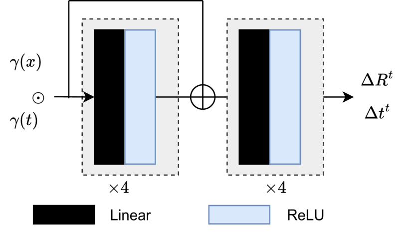
As depicted in Fig. 10, superpoint deformation network consists of 8-layer MLPs with a hidden dimension of 256, while the non-rigid deformation network consists of 4-layer MLPs with a hidden dimension of 64 and ReLU activations. Upon initializing and , the weights and bias of last layer are set to 0.
For the D-NeRF dataset, we initialize 3D Gaussians from random point clouds with 10k points. We apply densification and pruning to the 3D Gaussians every 100 iterations, starting from 600 iterations and stopping at 15k iterations. The opacity of 3D Gaussians is reset every 3k iterations until 15k iterations.
Concerning the real-world HyperNeRF Dataset, we utilize colmap to derive camera parameters and colored sparse point clouds. Densification and pruning of 3D Gaussians occur every 1000 iterations, starting from 1000 iterations and stopping at 15k iterations. The opacity of 3D Gaussians is reset every 6k iterations until 15k iterations.
Appendix B More about Real Time Rendering
We compare the rendering speed between our SP-GS and other methods on different GPUs (i.e. V100, TITAN Xp, GTX 1060). Results are shown in Table 7, Table 8 and Table 9. As can be seen from those tables, our SP-GS can achieve real-time rendering speed of complex scenes on devices with limited computing power (such as GTX 1060), while D-3D-GS cannot achieve real-time rendering.
| Method | V100 | TITAN Xp | GTX 1060 |
|---|---|---|---|
| NeRF-based | |||
| D-3D-GS | 45.05 | 30.84 | 13.44 |
| 4D-GS | 143.69 | 134.16 | 95.01 |
| SP-GS (ours) | 227.25 | 197.90 | 140.341 |
| Method | V100 | TITAN Xp | GTX 1060 |
|---|---|---|---|
| NeRF-based | |||
| D-3D-GS | 4.87 | 4.71 | 2.00 |
| 4D-GS | 66.21 | 58.95 | 29.03 |
| SP-GS (ours) | 117.86 | 101.58 | 56.06 |
| Method | V100 | TITAN Xp | GTX 1060 |
|---|---|---|---|
| NeRF-based | |||
| D-3D-GS | 15.27 | 13.13 | 7.33 |
| SP-GS (ours) | 251.70 | 160.06 | 90.40 |
Appendix C Per Scene Results
C.1 D-NeRF Dataset
On the synthetic D-NeRF dataset, Tab.16 illustrates per-scene quantitative comparisons in terms of PSNR, SSIM, and LPIPS (alex). Our approaches, SP-GS and SP-GS+NG, exhibit superior performance compared to non-Gaussian-Splatting based methods. In comparison to the concurrent work D-3D-GS (Yang et al., 2024), which employs heavy MLPs (8 layers, 256-D) on every single 3D Gaussian and cannot achieve real-time rendering, our results are slightly less favorable.
Tab. 10 elucidates the number of the final 3D Gaussians (#Gaussians), the training time (train), and the rendering speed (FPS) for SP-GS and SP-GS+NG on the D-NeRF dataset. It is evident that a reduced number of Gaussians result in faster training time and rendering speed. Therefore, adjusting hyper-parameters of the ”Adaptive Control of Gaussians” (e.g., densify and prune interval, threshold) is a possible way to achieve faster training time and rendering speed. It is worth noting that the training time of SP-GS+NG in table only includes the time of training the NG part, and does not include the training time for SP-GS.
C.2 HyperNeRF Dataset
For the HyperNeRF Dataset, Tab.17 reports the per scene results on vrig-broom, vrig-3dprinter, vrig-chichen and vrig-peel-banana. Tab. 11 elucidates the number of the final 3D Gaussians (#Gaussians), the training time (train), and the rendering speed (FPS) for SP-GS and SP-GS+NG on the HyperNeRF Dataset.
| scene | #Gaussians | SP-GS | SP-GS+NG | ||
|---|---|---|---|---|---|
| Train | FPS | Train | FPS | ||
| hellwarrior | 38k | 26m | 249.93 | +8m | 65.54 |
| mutant | 181k | 79m | 210.42 | +9m | 199.43 |
| hook | 135k | 60m | 230.35 | +8m | 107.82 |
| bouncingballs | 41k | 28m | 181.77 | +9m | 154.2 |
| lego | 264k | 113m | 168.89 | +16m | 45.32 |
| trex | 165k | 72m | 186.65 | +11m | 91.76 |
| standup | 74k | 38m | 260.34 | +8m | 155.6 |
| jumpingjack | 68k | 39m | 271.27 | +9m | 61.13 |
| average | 120k | 57m | 219.95 | +8.6m | 110.10 |
| scene | #Gaussians | SP-GS | SP-GS+NG | ||
|---|---|---|---|---|---|
| Train | FPS | Train | FPS | ||
| 3D Printer | 151K | 86m | 149.84 | +15m | 31.41 |
| Broom | 565K | 329m | 107.26 | +34m | 6.6 |
| Chicken | 153K | 71m | 146.04 | +11m | 22.24 |
| Peel Banana | 404K | 180m | 68.30 | +17m | 10.15 |
| average | 318K | 167m | 117.86 | +19m | 17.6 |
C.3 NeRF-DS Dataset.
For the NeRF-DS Dataset, Tab.18 reports the per scene results.
C.4 Dynamic Scene Dataset
We further compare our approach against other methods using the NVIDIA Dynamic Scene Dataset (Yoon et al., 2020), which is composed of 7 video sequences. These sequences are captured with 12 cameras (GoPro Black Edition) utilizing a static camera rig. All cameras concurrently capture images at 12 different time steps. Except for the densify and prune interval, we train our approaches on this dataset using the same configuration as the one employed for the HyperNeRF Dataset. In the initial 15k iterations, we densify 3D Gaussians every 1000 iterations, prune 3D Gaussians every 8000 iterations, and reset opacity every 3000 iterations.
Table 19 presents the results of quantitative comparisons. In comparison to state-of-the-art methods, our approach also exhibits competitive visual quality.
Appendix D Additional Experiments
In this section, we conduct additional experiments to investigate key components and factors utilized in our method, aiming to enhance our understand of the mechanism and illustrate its efficacy.
D.1 The Loss Weights
There are three hyperparameters (i.e., , , and ) to balance the weights of loss terms. As illustrated in Tab. 12, we conduct experiments to showcase the impact of these hyperparameters. It should be emphasized that denotes the exclusion of the respective loss term. The results indicate that there is only a minor effect when varying these hyperparameters over a large range ( to ).
| 0 | ||||||
|---|---|---|---|---|---|---|
| PSNR | 35.498 | 35.435 | 35.521 | 35.338 | 35.667 | 35.350 |
| SSIM | 0.9808 | 0.9807 | 0.9806 | 0.9810 | 0.9809 | 0.9809 |
| LPIPS | 0.0198 | 0.0200 | 0.0208 | 0.021 | 0.0202 | 0.0142 |
| 0 | ||||||
| PSNR | 35.542 | 35.483 | 35.379 | 35.509 | 35.552 | 35.551 |
| SSIM | 0.9819 | 0.9816 | 0.9813 | 0.9813 | 0.9819 | 0.9817 |
| LPIPS | 0.0128 | 0.0135 | 0.0130 | 0.0129 | 0.0126 | 0.0129 |
| 0 | ||||||
| PSNR | 35.418 | 35.431 | 35.567 | 35.682 | 35.315 | 35.561 |
| SSIM | 0.9813 | 0.9813 | 0.9816 | 0.9814 | 0.9813 | 0.9819 |
| LPIPS | 0.0138 | 0.0134 | 0.0131 | 0.0134 | 0.0135 | 0.0133 |
D.2 The Model Size
We investigate the impact of the model size of the superpoints deformation network . We manipulate the network width (i.e., the dimensions of hidden neurons) and the network depth (i.e., the number of hidden layers), presenting results on the D-NeRF dataset in Table 13. Following NeRF (Mildenhall et al., 2020), when the network depth exceeds 4, we introduce a skip connection between the inputs and the 5th fully-connected layer. With the exception of the configuration with width=64 and depth=5, which exhibits diminished performance due to the skip concatenation, the experimental results clearly demonstrate that a larger leads to a higher visual quality. Since we only need to predict the deformation of superpoints, increasing the model size will results in only a modest rise in computational expense during training. Therefore, employing a larger superpoints deformation network is a viable option to enhance the visual quality of dynamic scenes.
| width | depth | PSNR | SSIM | LIPIS |
|---|---|---|---|---|
| 64 | 1 | 34.7360 | 0.9797 | 0.0152 |
| 64 | 2 | 35.3632 | 0.9814 | 0.0139 |
| 64 | 3 | 35.5986 | 0.9818 | 0.0131 |
| 64 | 4 | 35.3418 | 0.9803 | 0.0142 |
| 64 | 5 | 27.2319 | 0.9491 | 0.0586 |
| 64 | 6 | 35.4901 | 0.9813 | 0.0139 |
| 64 | 7 | 35.7497 | 0.9818 | 0.0130 |
| 64 | 8 | 35.8021 | 0.9823 | 0.0128 |
| 128 | 8 | 36.1375 | 0.9838 | 0.0126 |
| 256 | 8 | 36.4452 | 0.9837 | 0.0123 |
D.3 Warm-up Train Stage
To train SP-GS model for a dynamic scene, there is a warm up training stage, i.e. we do not train the superpoint deformation network and apply deformation to Gaussians in the first 3k iterations. The stage will generate a coarse shape, which is important for initialization of superpoints. The quantity results on D-NeRF dataset in Table 14 illustrate the the importance of warm up.
| PSNR | SSIM | LPIPS | |
|---|---|---|---|
| w/o warm up | 21.56 | 0.8979 | 0.1445 |
| w warm-up | 37.98 | 0.9876 | 0.0164 |
D.4 Inference
There are two way to rendering images during inference, i.e., using network or interpolation. Table 15 demonstrates that two way have almost same visual quality, but the FPS of using is lower than the FPS using interpolation, i.e. 168.01 vs. 219.95.
| PSNR | SSIM | LPIPS | FPS | |
|---|---|---|---|---|
| using , Eq. 6 | 36.2281 | 0.9815 | 0.0124 | 168.01 |
| interp, Eq. 8 | 36.2280 | 0.9815 | 0.0124 | 219.95 |
| Methods | Hell Warrior | Mutant | Hook | Bouncing Balls | ||||||||
|---|---|---|---|---|---|---|---|---|---|---|---|---|
| PSNR | SSIM | LPIPS | PSNR | SSIM | LPIPS | PSNR | SSIM | LPIPS | PSNR | SSIM | LPIPS | |
| D-NeRF (Pumarola et al., 2021) | 24.06 | 0.9440 | 0.0707 | 30.31 | 0.9672 | 0.0392 | 29.02 | 0.9595 | 0.0546 | 38.17 | 0.9891 | 0.0323 |
| TiNeuVox (Fang et al., 2022) | 27.10 | 0.9638 | 0.0768 | 31.87 | 0.9607 | 0.0474 | 30.61 | 0.9599 | 0.0592 | 40.23 | 0.9926 | 0.0416 |
| Tensor4D (Shao et al., 2022) | 31.26 | 0.9254 | 0.0735 | 29.11 | 0.9451 | 0.0601 | 28.63 | 0.9433 | 0.0636 | 24.47 | 0.9622 | 0.0437 |
| K-Planes (Fridovich-Keil et al., 2023) | 24.58 | 0.9520 | 0.0824 | 32.50 | 0.9713 | 0.0362 | 28.12 | 0.9489 | 0.0662 | 40.05 | 0.9934 | 0.0322 |
| HexPlane (Cao & Johnson, 2023) | 24.24 | 0.94 | 0.07 | 33.79 | 0.98 | 0.03 | 28.71 | 0.96 | 0.05 | 39.69 | 0.99 | 0.03 |
| Ti-DNeRF (Park et al., 2023) | 25.40 | 0.953 | 0.0682 | 34.70 | 0.983 | 0.0226 | 28.76 | 0.960 | 0.0496 | 43.32 | 0.996 | 0.0203 |
| 3D-GS (Kerbl et al., 2023) | 29.89 | 0.9143 | 0.1113 | 24.50 | 0.9331 | 0.0585 | 21.70 | 0.8864 | 0.1040 | 23.20 | 0.9586 | 0.0608 |
| D-3D-GS (Yang et al., 2024) | 41.41 | 0.9870 | 0.0115 | 42.61 | 0.9950 | 0.0020 | 37.09 | 0.9858 | 0.0079 | 40.95 | 0.9953 | 0.0027 |
| 4D-GS (Wu et al., 2024) | 28.77 | 0.9729 | 0.0241 | 37.43 | 0.9874 | 0.0092 | 33.01 | 0.9763 | 0.0163 | 40.78 | 0.9942 | 0.0060 |
| SP-GS (ours) | 40.19 | 0.9894 | 0.0066 | 39.43 | 0.9868 | 0.0164 | 35.36 | 0.9804 | 0.0187 | 40.53 | 0.9831 | 0.0326 |
| SP-GS+NG(ours) | 39.01 | 0.9938 | 0.0043 | 41.02 | 0.9890 | 0.0112 | 35.35 | 0.9827 | 0.0138 | 41.65 | 0.9762 | 0.0278 |
| Methods | Lego | T-Rex | Stand Up | Jumping Jacks | ||||||||
| PSNR | SSIM | LPIPS | PSNR | SSIM | LPIPS | PSNR | SSIM | LPIPS | PSNR | SSIM | LPIPS | |
| D-NeRF (Pumarola et al., 2021) | 25.56 | 0.9363 | 0.0821 | 30.61 | 0.9671 | 0.0535 | 33.13 | 0.9781 | 0.0355 | 32.70 | 0.9779 | 0.0388 |
| TiNeuVox (Fang et al., 2022) | 26.64 | 0.9258 | 0.0877 | 31.25 | 0.9666 | 0.0478 | 34.61 | 0.9797 | 0.0326 | 33.49 | 0.9771 | 0.0408 |
| Tensor4D (Shao et al., 2022) | 23.24 | 0.9183 | 0.0721 | 23.86 | 0.9351 | 0.0544 | 30.56 | 0.9581 | 0.0363 | 24.20 | 0.9253 | 0.0667 |
| K-Planes (Fridovich-Keil et al., 2023) | 28.91 | 0.9695 | 0.0331 | 30.43 | 0.9737 | 0.0343 | 33.10 | 0.9793 | 0.0310 | 31.11 | 0.9708 | 0.0468 |
| TI-DNeRF (Park et al., 2023) | 25.33 | 0.943 | 0.0413 | 33.06 | 0.982 | 0.0212 | 36.27 | 0.988 | 0.0159 | 35.03 | 0.985 | 0.0249 |
| HexPlane (Cao & Johnson, 2023) | 25.22 | 0.94 | 0.04 | 30.67 | 0.98 | 0.03 | 34.36 | 0.98 | 0.02 | 31.65 | 0.97 | 0.04 |
| 3D-GS (Kerbl et al., 2023) | 23.04 | 0.9288 | 0.0521 | 21.91 | 0.9536 | 0.0552 | 21.91 | 0.9299 | 0.0893 | 20.64 | 0.9292 | 0.1065 |
| D-3D-GS (Yang et al., 2024) | 24.91 | 0.9426 | 0.0299 | 37.67 | 0.9929 | 0.0041 | 44.30 | 0.9947 | 0.0031 | 37.59 | 0.9893 | 0.0085 |
| 4D-GS (Wu et al., 2024) | 25.04 | 0.9362 | 0.0382 | 33.61 | 0.9828 | 0.0136 | 38.11 | 0.9896 | 0.0072 | 35.44 | 0.9853 | 0.0127 |
| SP-GS (ours) | 24.48 | 0.9390 | 0.0331 | 32.69 | 0.9861 | 0.0243 | 42.07 | 0.9926 | 0.0096 | 35.56 | 0.9950 | 0.0069 |
| SP-GS+NG (ours) | 28.58 | 0.9518 | 0.0331 | 34.47 | 0.9839 | 0.0182 | 42.12 | 0.9925 | 0.0065 | 34.32 | 0.9959 | 0.0064 |
| Methods | Broom | 3D Printer | Chicken | Peel banana | Mean | ||||||||||
|---|---|---|---|---|---|---|---|---|---|---|---|---|---|---|---|
| PSNR | MS-SSIM | LIPIS | PSNR | MS-SSIM | LIPIS | PSNR | MS-SSIM | LIPIS | PSNR | MS-SSIM | LIPIS | PSNR | MS-SSIM | LIPIS | |
| NeRF (Mildenhall et al., 2020) | 19.9 | 0.653 | 0.692 | 20.7 | 0.780 | 0.357 | 19.9 | 0.777 | 0.325 | 20.0 | 0.739 | 0.413 | 20.1 | 0.735 | 0.424 |
| NV (Lombardi et al., 2019) | 17.7 | 0.623 | 0.360 | 16.2 | 0.665 | 0.330 | 17.6 | 0.615 | 0.336 | 15.9 | 0.380 | 0.413 | 16.9 | 0.571 | - |
| NSFF (Li et al., 2021b) | 26.1 | 0.871 | 0.284 | 27.7 | 0.947 | 0.125 | 26.9 | 0.944 | 0.106 | 24.6 | 0.902 | 0.198 | 26.3 | 0.916 | - |
| Nerfies (Park et al., 2021a) | 19.2 | 0.567 | 0.325 | 20.6 | 0.830 | 0.108 | 26.7 | 0.943 | 0.0777 | 22.4 | 0.872 | 0.147 | 22.2 | 0.803 | - |
| HyperNeRF (Park et al., 2021b) | 19.3 | 0.591 | 0.296 | 20.0 | 0.821 | 0.111 | 26.9 | 0.948 | 0.0787 | 23.3 | 0.896 | 0.133 | 22.4 | 0.814 | - |
| TiNeuVox-S (Fang et al., 2022) | 21.9 | 0.707 | - | 22.7 | 0.836 | - | 27.0 | 0.929 | - | 22.1 | 0.780 | - | 23.4 | 0.813 | - |
| TiNeuVox-B (Fang et al., 2022) | 21.5 | 0.686 | - | 22.8 | 0.841 | - | 28.3 | 0.947 | - | 24.4 | 0.873 | - | 24.3 | 0.837 | - |
| NDVG (Guo et al., 2022) | 22.4 | 0.839 | - | 21.5 | 0.703 | - | 27.1 | 0.939 | - | 22.8 | 0.828 | - | 23.3 | 0.823 | - |
| TI-DNeRF (Park et al., 2023) | 20.48 | 0.685 | - | 20.38 | 0.678 | - | 21.89 | 0.869 | - | 28.87 | 0.965 | - | 24.35 | 0.866 | - |
| NeRFPlayer (Song et al., 2022) | 21.7 | 0.635 | - | 22.9 | 0.810 | - | 26.3 | 0.905 | - | 24.0 | 0.863 | - | 23.7 | 0.803 | - |
| 3D-GS (Kerbl et al., 2023) | 19.74 | 0.4949 | 0.3745 | 19.26 | 0.6686 | 0.4281 | 22.51 | 0.7954 | 0.3307 | 19.54 | 0.6688 | 0.2339 | 20.26 | 0.6569 | 0.3418 |
| 4D-GS (Wu et al., 2024) | 22.01 | 0.6883 | 0.5448 | 21.98 | 0.8038 | 0.2763 | 27.58 | 0.9333 | 0.1468 | 28.52 | 0.9254 | 0.198 | 25.02 | 0.8377 | 0.2915 |
| SP-GS (ours) | 20.07 | 0.6004 | 0.3430 | 24.31 | 0.8719 | 0.2312 | 30.81 | 0.9550 | 0.1262 | 27.23 | 0.9341 | 0.1286 | 25.61 | 0.8404 | 0.2073 |
| SP-GS+NR (ours) | 22.76 | 0.7794 | 0.2812 | 24.88 | 0.8836 | 0.2100 | 31.47 | 0.9609 | 0.1122 | 28.01 | 0.9442 | 0.1186 | 26.78 | 0.8920 | 0.1805 |
| Method | Sieve | Plate | Bell | Press | ||||||||
|---|---|---|---|---|---|---|---|---|---|---|---|---|
| PSNR | MS-SSIM | LPIPS | PSNR | MS-SSIM | LPIPS | PSNR | MS-SSIM | LPIPS | PSNR | MS-SSIM | LPIPS | |
| TiNeuVox | 21.49 | 0.8265 | 0.3176 | 20.58 | 0.8027 | 0.3317 | 23.08 | 0.8242 | 0.2568 | 24.47 | 0.8613 | 0.3001 |
| HyperNeRF | 25.43 | 0.8798 | 0.1645 | 18.93 | 0.7709 | 0.2940 | 23.06 | 0.8097 | 0.2052 | 26.15 | 0.8897 | 0.1959 |
| NeRF-DS | 25.78 | 0.8900 | 0.1472 | 20.54 | 0.8042 | 0.1996 | 23.19 | 0.8212 | 0.1867 | 25.72 | 0.8618 | 0.2047 |
| 3D-GS | 23.16 | 0.8203 | 0.2247 | 16.14 | 0.6970 | 0.4093 | 21.01 | 0.7885 | 0.2503 | 22.89 | 0.8163 | 0.2904 |
| D-3D-GS | 25.01 | 0.867 | 0.1509 | 20.16 | 0.8037 | 0.2243 | 25.38 | 0.8469 | 0.1551 | 25.59 | 0.8601 | 0.1955 |
| SP-GS(ours) | 25.62 | 0.8651 | 0.1631 | 18.91 | 0.7725 | 0.2767 | 25.20 | 0.8430 | 0.1704 | 24.34 | 0.846 | 0.2157 |
| SP-GS+NG(ours) | 25.39 | 0.8599 | 0.1667 | 19.81 | 0.7849 | 0.2538 | 24.97 | 0.8421 | 0.1782 | 24.93 | 0.861 | 0.2073 |
| Method | Cup | As | Basin | Mean | ||||||||
| PSNR | MS-SSIM | LPIPS | PSNR | MS-SSIM | LPIPS | PSNR | MS-SSIM | LPIPS | PSNR | MS-SSIM | LPIPS | |
| TiNeuVox | 19.71 | 0.8109 | 0.3643 | 21.26 | 0.8289 | 0.3967 | 20.66 | 0.8145 | 0.2690 | 21.61 | 0.8234 | 0.2766 |
| HyperNeRF | 24.59 | 0.8770 | 0.1650 | 25.58 | 0.8949 | 0.1777 | 20.41 | 0.8199 | 0.1911 | 23.45 | 0.8488 | 0.1990 |
| NeRF-DS | 24.91 | 0.8741 | 0.1737 | 25.13 | 0.8778 | 0.1741 | 19.96 | 0.8166 | 0.1855 | 23.60 | 0.8494 | 0.1816 |
| 3D-GS | 21.71 | 0.8304 | 0.2548 | 22.69 | 0.8017 | 0.2994 | 18.42 | 0.7170 | 0.3153 | 20.29 | 0.7816 | 0.2920 |
| D-3D-GS | 24.54 | 0.8848 | 0.1583 | 26.15 | 0.8816 | 0.1829 | 19.61 | 0.7879 | 0.1897 | 23.78 | 0.8474 | 0.1795 |
| SP-GS(ours) | 24.43 | 0.8823 | 0.1728 | 24.44 | 0.8626 | 0.2255 | 19.09 | 0.7627 | 0.2189 | 23.15 | 0.8335 | 0.2062 |
| SP-GS+NG(ours) | 23.66 | 0.8738 | 0.1853 | 25.16 | 0.8650 | 0.2246 | 19.36 | 0.7667 | 0.2429 | 23.33 | 0.8362 | 0.2084 |
| Methods | Jumping | Skating | Truck | Umbrella | ||||||||
|---|---|---|---|---|---|---|---|---|---|---|---|---|
| PSNR | SSIM | LPIPS | PSNR | SSIM | LPIPS | PSNR | SSIM | LPIPS | PSNR | SSIM | LPIPS | |
| NeRF (Mildenhall et al., 2020)+time | 16.72 | 0.42 | 0.489 | 19.23 | 0.46 | 0.542 | 17.17 | 0.39 | 0.403 | 17.17 | - | 0.752 |
| D-NeRF (Pumarola et al., 2021) | 21.0 | 0.68 | 0.21 | 20.8 | 0.62 | 0.35 | 22.9 | 0.71 | 0.15 | - | - | - |
| NR-NeRF (Tretschk et al., 2021) | 19.38 | 0.61 | 0.295 | 23.29 | 0.72 | 0.234 | 19.02 | 0.44 | 0.453 | 19.26 | - | 0.427 |
| HyperNeRF (Park et al., 2021b) | 17.1 | 0.45 | 0.32 | 20.6 | 0.58 | 0.19 | 19.4 | 0.43 | 0.21 | - | - | - |
| TiNeuVox (Fang et al., 2022) | 19.7 | 0.60 | 0.26 | 21.9 | 0.68 | 0.16 | 22.9 | 0.63 | 0.19 | - | - | - |
| NSFF (Li et al., 2021b) | 24.12 | 0.80 | 0.144 | 28.90 | 0.88 | 0.124 | 25.94 | 0.76 | 0.171 | 22.58 | - | 0.302 |
| DVS (Gao et al., 2021) | 23.23 | 0.83 | 0.144 | 28.90 | 0.94 | 0.124 | 25.78 | 0.86 | 0.134 | 23.15 | - | 0.146 |
| RoDynRF (Liu et al., 2023) | 25.66 | 0.84 | 0.071 | 28.68 | 0.93 | 0.040 | 29.13 | 0.89 | 0.063 | 24.26 | - | 0.063 |
| Point-DynRF (Park & Kim, 2024) | 23.6 | 0.90 | 0.14 | 29.6 | 0.96 | 0.04 | 28.5 | 0.94 | 0.08 | - | - | - |
| SP-GS (ours) | 22.13 | 0.7484 | 0.4675 | 29.21 | 0.9079 | 0.2360 | 27.38 | 0.8401 | 0.1898 | 24.88 | 0.6568 | 0.3231 |
| SP-GS+NG(ours) | 23.41 | 0.8104 | 0.3267 | 29.54 | 0.9124 | 0.2323 | 27.62 | 0.8440 | 0.1860 | 25.18 | 0.6617 | 0.3200 |
| Methods | Balloon1 | Balloon2 | Playground | Avg | ||||||||
| PSNR | SSIM | LPIPS | PSNR | SSIM | LPIPS | PSNR | SSIM | LPIPS | PSNR | SSIM | LPIPS | |
| NeRF (Mildenhall et al., 2020)+time | 17.33 | 0.40 | 0.304 | 19.67 | 0.54 | 0.236 | 13.80 | 0.18 | 0.444 | 17.30 | 0.40 | 0.453 |
| D-NeRF (Pumarola et al., 2021) | 18.0 | 0.44 | 0.28 | 19.8 | 0.52 | 0.30 | 19.4 | 0.65 | 0.17 | 20.4 | 0.59 | 0.24 |
| NR-NeRF (Tretschk et al., 2021) | 16.98 | 0.34 | 0.225 | 22.23 | 0.70 | 0.212 | 14.24 | 0.19 | 0.336 | 19.20 | 0.50 | 0.330 |
| HyperNeRF (Park et al., 2021b) | 12.8 | 0.13 | 0.56 | 15.4 | 0.20 | 0.44 | 12.3 | 0.11 | 0.52 | 16.3 | 0.32 | 0.37 |
| TiNeuVox (Fang et al., 2022) | 16.2 | 0.34 | 0.37 | 18.1 | 0.41 | 0.29 | 12.6 | 0.14 | 0.46 | 18.6 | 0.47 | 0.29 |
| NSFF (Li et al., 2021b) | 21.40 | 0.69 | 0.225 | 24.09 | 0.73 | 0.228 | 20.91 | 0.70 | 0.220 | 23.99 | 0.76 | 0.205 |
| DVS (Gao et al., 2021) | 21.47 | 0.75 | 0.125 | 25.97 | 0.85 | 0.059 | 23.65 | 0.85 | 0.093 | 24.74 | 0.85 | 0.118 |
| RoDynRF (Liu et al., 2023) | 22.37 | 0.76 | 0.103 | 26.19 | 0.84 | 0.054 | 24.96 | 0.89 | 0.048 | 25.89 | 0.86 | 0.065 |
| Point-DynRF (Park & Kim, 2024) | 21.7 | 0.88 | 0.12 | 26.2 | 0.92 | 0.06 | 22.2 | 0.91 | 0.09 | 25.3 | 0.92 | 0.08 |
| SP-GS (ours) | 24.36 | 0.8783 | 0.1802 | 29.65 | 0.9059 | 0.0965 | 22.29 | 0.7721 | 0.2338 | 25.70 | 0.8156 | 0.2467 |
| SP-GS+NG(ours) | 24.96 | 0.8811 | 0.1808 | 26.31 | 0.7882 | 0.2291 | 20.28 | 0.7453 | 0.3488 | 25.33 | 0.8062 | 0.2605 |