Superluminal Motion-Assisted 4-Dimensional Light-in-Flight Imaging
Abstract
Advances in high speed imaging techniques have opened new possibilities for capturing ultrafast phenomena such as light propagation in air or through media. Capturing light-in-flight in 3-dimensional -space has been reported based on various types of imaging systems, whereas reconstruction of light-in-flight information in the fourth dimension has been a challenge. We demonstrate the first 4-dimensional light-in-flight imaging based on the observation of a superluminal motion captured by a new time-gated megapixel single-photon avalanche diode camera. A high resolution light-in-flight video is generated with no laser scanning, camera translation, interpolation, nor dark noise subtraction. A machine learning technique is applied to analyze the measured spatio-temporal data set. A theoretical formula is introduced to perform least-square regression, and extra-dimensional information is recovered without prior knowledge. The algorithm relies on the mathematical formulation equivalent to the superluminal motion in astrophysics, which is scaled by a factor of a quadrillionth. The reconstructed light-in-flight trajectory shows a good agreement with the actual geometry of the light path. Our approach could potentially provide novel functionalities to high speed imaging applications such as non-line-of-sight imaging and time-resolved optical tomography.
I INTRODUCTION
Progress in high speed imaging techniques has enabled observation and recording of light propagation dynamics in free space as well as in transparent, translucent and scattering media. Various approaches for capturing the light-in-flight have been demonstrated: holographic techniques [1, 2, 3], photonic mixers [4], time-encoded amplified imaging [5], streak cameras [6, 7], intensified CCDs [8] and silicon CMOS image sensors [9]. In recent years, 1- and 2-dimensional arrays of single-photon avalanche diode (SPAD) have been adopted for the light-in-flight imaging systems [10, 11, 12, 13, 14, 15]. These sensors boost data acquisition speed by employing pixel-parallel detection of time stamping with picosecond time resolution and single-photon sensitivity. However, the sensors are capable of sampling only 3-dimensional spatio-temporal information (, , ) of the target light, and hence the tracking of light-in-flight breaking outside a -plane is a challenge.
A method to reconstruct an extra-dimensional position information, , from measured spatio-temporal information has been recently investigated by researchers [16]. The authors remark that different propagation angle with respect to -plane results in the different apparent velocity of light. Thus, comparing the measured spatio-temporal data set with this theory could give an estimation of -component in the light propagation vector. Yet, the analysis is limited to a simplified case with single straight light paths within -plane passing a fixed point, and complete 4-dimensional reconstruction of light-in-flight in arbitrary paths remains to be verified. In addition, spatial resolution of the detector array is critical for accurate reconstruction of the 4-dimensional trace; the reported SPAD sensor resolutions, e.g. 6432 [15], 3232 [10] and 2561 [13] pixels, are not sufficient, whereas significant improvement of the estimation error for (, , , ) is expected with orders of magnitude larger arrays, typically in the megapixels. CMOS sensors routinely achieve megapixel resolutions, e.g. 0.3 Mpixel resolution is reported for high speed imaging [9], however the necessary timing resolution is not reached and it is limited to 10 nanoseconds.
In this paper we demonstrate the 4-dimensional light-in-flight imaging based on the first time-gated megapixel SPAD camera [17]. In contrast to conventional time-correlated single-photon counting (TCSPC) approaches, where power- and area-consuming time-to-digital converter (TDC) circuits restrict the scaling of the pixel array [18, 19, 20], our time-gating approach [17] achieves a much more compact pixel circuit, suitable for large-scale arrays. Our camera achieves a megapixel format, while, at the same time ensuring a time resolution comparable to that of a TDC. Owing to an unprecedented high spatio-temporal resolution, a superluminal motion of laser pulse was successfully captured in a frame sequence. We then introduced a theoretical equation to fit the measured data set in 3-dimensional space. A 4-dimensional point cloud is computationally reproduced without prior knowledge, exhibiting a good agreement with the actual light propagation vectors.
II PRINCIPLE AND EXPERIMENTAL SETUP
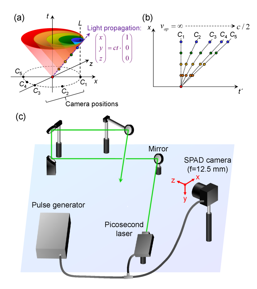
To illustrate our method, we introduce a Minkowski space that is describing the spatio-temporal propagation of a laser pulse and scattered photons towards fixed observation points. Fig. 1(a) shows a schematic illustration of light-in-flight observation in the Minkowski space at = 0. A straight light propagation along -axis is depicted as (, , ) = (, 0, 0), where is the speed of light. In the Minkowski space, this equation corresponds to a single tilted line crossing the origin (purple arrow in Figure 1(a)). A camera is located at the position ( = 1,2,…,5). The observation of the light-in-flight at the camera is mediated by scattered light at each point on the path (colored dots on the purple arrow). The propagation of the scattered light from the points are described as light cones. Here we define t as the time at which the light propagating from a laser source reaches a point (, , ), called scattering point on the light path, and as a time at which the light scattered by the medium at (, , ) reaches the camera. Due to the finite speed of light, a time difference from to is proportional to the spatial distance between the scattering point and the camera location. In Minkowski space, the observation time can be visualized as an intersection point of the light cone and a vertical line passing (dotted line). The relation between the light position and the corresponding observation time is shown in Figure 1(b). The behavior is highly dependent on the camera position with respect to the scattering point, i.e. at certain points it appears to be faster than in others. For example, at where the light is coming towards the camera, the scattering light from all the points on the light path reaches the camera at the same time. The corresponding apparent velocity, defined as = , is infinite, or appears not to change irrespective of the distance of the scattering point (, , ) from the camera. At , in contrast, the light propagating away from the camera is observed with the apparent velocity of /2. For other scattering points corresponding to relative camera positions , , and , one observes intermediate apparent velocities, depending on the relative position and angle of the line of sight between scattering point and camera. Hence, analyzing the apparent velocity provides an estimated light propagation vector with extra-dimensional information. The discussion can be generalized for higher dimensions; the detailed analysis of measured (, , ) data set and its local apparent velocity would enable a 4-dimensional reconstruction of the light-in-flight history. A 2D-projected intuitive visualization for the propagation of scattered light is provided in Supplementary Video 1. Note that angle-dependent apparent velocity of light can be seen in nature, for instance in an astronomical phenomenon called superluminal motion. In this case, relativistic jets of matter are emitted from radio galaxies, quasars, and other celestial objects, appearing to travel faster than light to the observer in a time scale of months to years. Light echoes are also known to produce superluminal motion [21, 22].
Fig. 1(c) is the experimental setup to verify the 4-dimensional light-in-flight imaging. A 510 nm-laser (average power: 2 mW, frequency: 40 MHz, optical pulse width: 130 ps, PicoQuant GmbH, Berlin, Germany) and the megapixel SPAD camera are synchronized by a pulse generator. The emitted laser pulses are reflected by four mirrors to construct a 3-dimensional trajectory. The megapixel SPAD camera can be operated in intensity imaging mode to capture the background scene and in time gating mode to capture laser propagation [17].
III 3-DIMENSIONAL LIGHT-IN-FLIGHT IMAGING
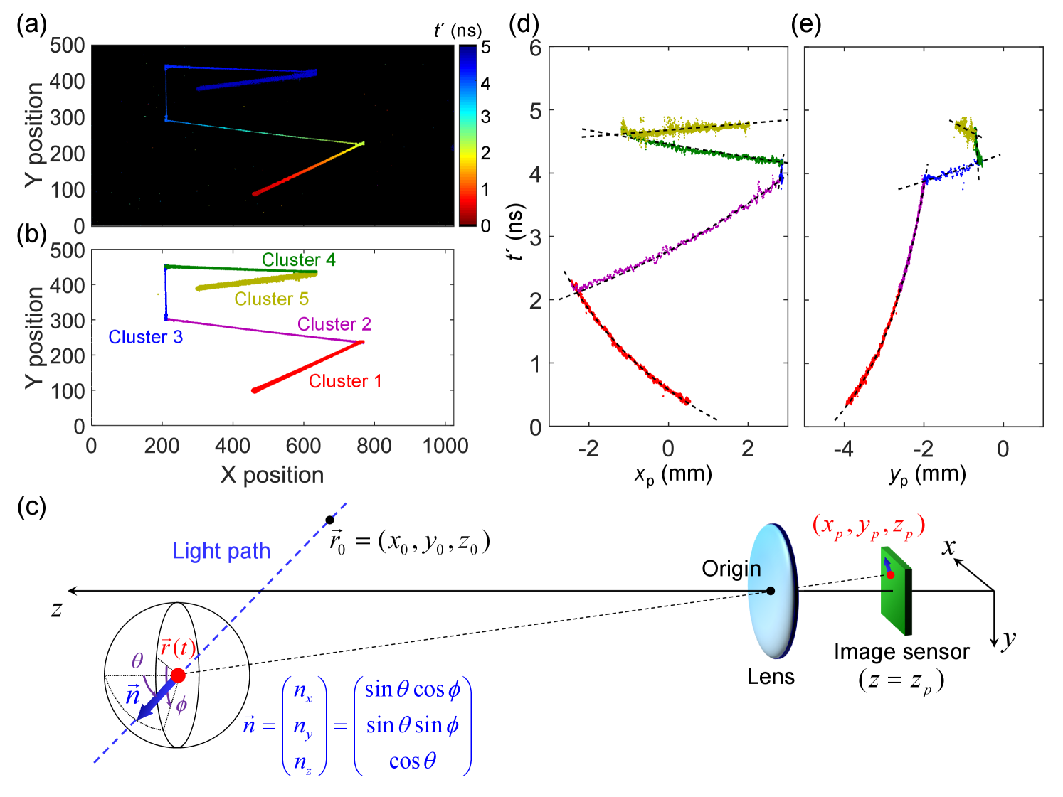
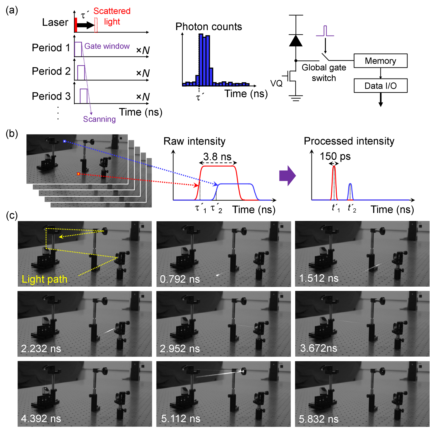
Fig. 2(a) describes the principle of time gate scanning method. A 3.8 ns global gate window is synchronized to a pulsed laser source. The pixels detect only photons impinging during the gate window. The gate position can be scanned with a gate shift of 36 ps relative to the laser pulse. At each gate position, 255 binary photon-counting frames are summed to form an 8-bit image. 250 slices of 8-bit images with the scanned time-gating window position over 9 ns range are used to extract the timing information of impinging photons. The gate window is defined by sending a short electrical pulse to the gate switch in the pixels. The data acquisition time for full gate scanning (250 slices) is 15 to 30 seconds, much shorter than in previous works (e.g. hours [6, 7] to 10 minutes [10]). This can be potentially reduced further by introducing a higher power laser.
Fig. 2(b) shows the procedure to generate a 3-dimensional light-in-flight video. The captured 250 slices of time-gating images form a photon intensity distribution for each pixel as a function of gate position. A rising edge position and “high” level of photon intensity in the intensity profile can be extracted for each pixel. Time-of-arrival information over the array is obtained by subtracting independently measured pixel-position-dependent timing skew from . The intensity profile is given as a convolution of the arriving photon distribution and the gating profile, and the laser pulse width appears to be elongated by 3.8 ns in the raw intensity profile. Analogously to a previously reported temporal deconvolution technique [10], the laser pulse width can be narrowed to the picosecond scale by replacing the intensity profile with a Gaussian distribution having a mean value of , standard deviation of 150 ps (corresponding to the combined jitter of laser and detector), and integrated photon counts of . Fig. 2(c) shows the selected frames of a reconstructed 3-dimensional light-in-flight video, where each frame is superimposed with a 2-dimensional intensity image independently captured by the same SPAD camera. A laser pulse starts to be observed around = 0 ns, is reflected by multiple mirrors, and goes out of sight around = 5.832 ns. The laser beam at = 5.112 ns appears to be stretched compared to the beam at = 2.232 ns. This implies an enhanced apparent velocity of the beam coming towards the camera at = 5.112 ns. Note that our system requires no mechanical laser scanning, spatial interpolation and dark noise image subtraction owing to its high spatial resolution array and low dark count rate [17]. A full 3-dimensional light-in-flight video with the frame interval of 36 ps is available in Supplementary Video 2.
IV 4-DIMENSIONAL RECONSTRUCTION OF LIGHT-IN-FLIGHT
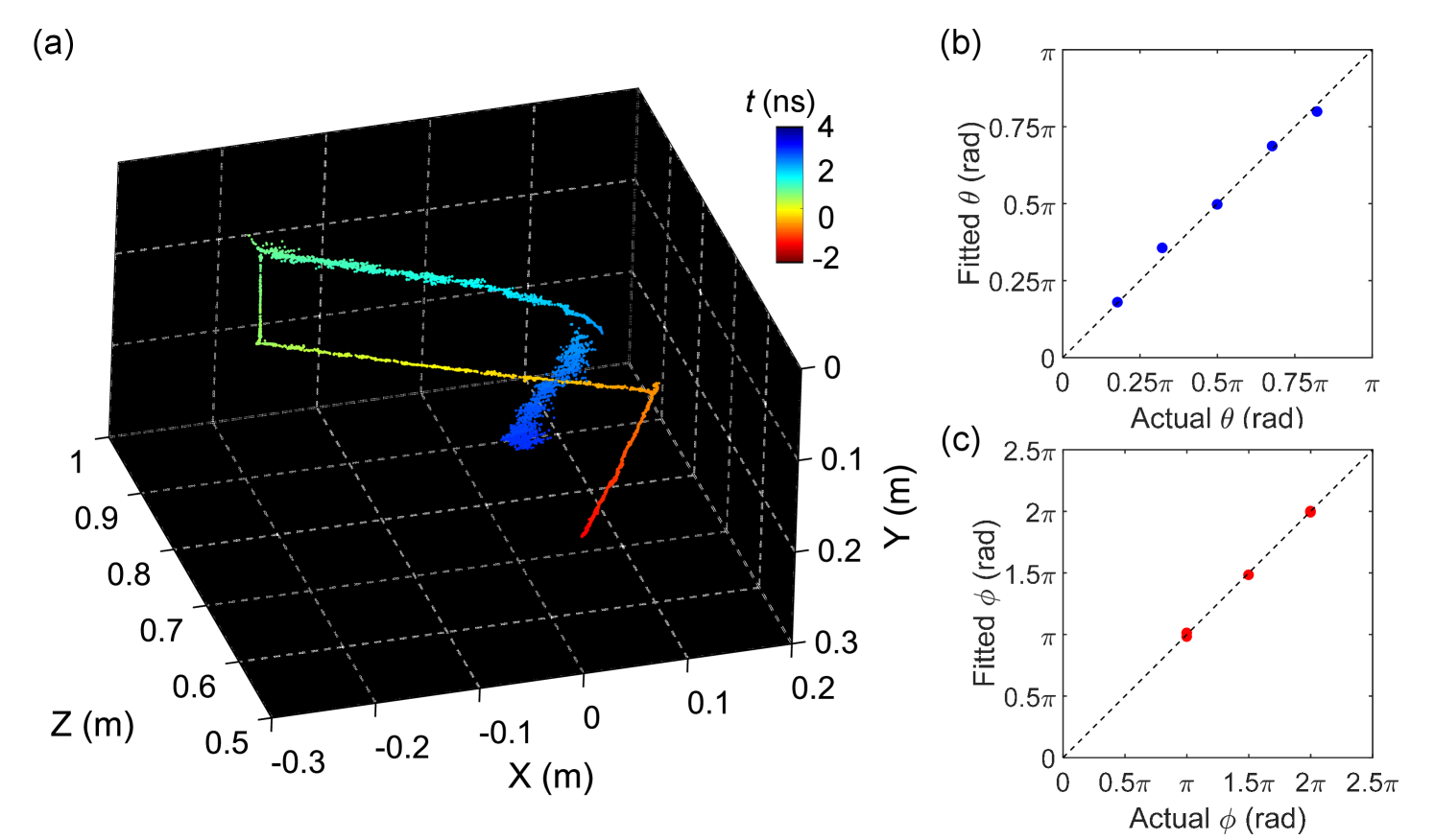
Fig. 3(a) shows a color-coded plot of the observation time for the propagating light. To reconstruct 4-dimensional light path, the data set needs to be subdivided into straight paths. We adopted the 2D Gaussian mixture model (GMM) fitting for data clustering, which is a common unsupervised machine learning technique. Fig. 3(b) shows the data points separated into five clusters. Note that the data clustering is performed based on 2-dimensional spatial information ( and ), whereas the time information is not taken into account.
Fig. 3(c) depicts the coordinate system for the light-in-flight analysis. Here we derive a theoretical formula to perform the least square regression for estimation of 4-dimensional light trajectory:
| (1) |
| (2) |
where is the total number of measurement data points, (, ) the corresponding pixel position on the focal plane for -th data point, the focal length (12.5mm), the measured observation time for -th data point, the position of the beam at = 0, and the normalized light propagation vector is represented as using a polar coordinate system. A single straight light trajectory can be expressed as , defined by five fitting parameters, , , , , . Those parameters are estimated by solving the above optimization problem for each data cluster.
Fig. 3(d) and 3(e) show the measured observation time as a function of and , where (, ) is the position of the pixel on the focal plane. Different colors of the data points correspond to the different data clusters. The result of fitting for each data cluster is shown as a dashed line, exhibiting a good agreement with the measured points for both and . Note that the fitting involves five independent parameters and is sensitive to the variation of the data. Hence, the spatio-temporal resolution of the camera is a critical factor determining the accuracy of the 4-dimensional reconstruction.
As shown in Fig. 4(a), the 4-dimensional point cloud is reconstructed without prior knowledge. The time evolution t of the beam is shown as colors of points, having a certain offset from the observation time due to the finite traveling time from the scattering point to the camera. The fully-recovered 4-dimensional information for each point enables the visualization of the point cloud from arbitrary viewpoint apart from the actual location of the SPAD camera. In contrast to the 3-dimensional light-in-flight video where the apparent velocity of light changes as a function of propagation angle, the 4-dimensional point cloud indicates the uniform speed of light irrespective of the beam position and angle. Relatively larger variation of the data points is observed for cluster 4 and 5. This originates from the enhanced apparent velocity of light coming towards the camera, leading to the reduced fitting accuracy and increased deviation.
The accuracy of the reconstruction is evaluated in Fig. 4(b) and 4(c). The figures show the fitted light propagation angles and as a function of the actual geometrical angles. Five dots correspond to the fitting results of the five data clusters. All the dots are along with the ideal trend (dashed line), indicating that the fitting results are in good agreement with the actual light propagation vectors.
Detailed analysis of the reconstruction performance for various parameter combinations is investigated based on Monte Carlo simulation in the Supplementary Note. The simulation shows that with the horizontal resolution of 1024 pixels, the estimation errors of the fitting parameters improve by a factor of 6 to 9 with respect to previously reported 3232 pixel SPAD cameras, thereby justifying the necessity of megapixel resolution for high-precision 4-dimensional light-in-flight imaging. The results also suggest that a further increase of the pixel array size could have a non-negligible impact on the stability and accuracy of light-in-flight measurements, along with the potential of further expansion of the measurement in distance and field-of-view.
V DISCUSSION
Our approach of reconstructing extra-dimensional light-in-flight information with high spatio-temporal resolution single-photon camera can be applied to a wide range of high-speed imaging techniques. One of the promising applications is the non-line-of-sight imaging [23, 24, 25, 26, 27]; by extending our approach for concentrated linear beam towards a diffused light, hidden objects can potentially be imaged with more simplified setup. The technique could also be used for imaging around and behind obstructing objects. Another potential application is the combination with optical tomography technique [28, 29, 30]; generalization of our theory can be useful for non-invasive 3-dimensional monitoring inside a target object structure as well as non-destructive measurement of 3-dimensional distribution of physical parameters such as refractive index and transmittance.
APPENDIX: DERIVATION OF THEORETICAL FORMULA FOR LEAST SQUARE REGRESSION
Time evolution of laser pulse position can be described as , where is the time-independent constant vector, the speed of light in vacuum, and the normalized vector representing the direction of light propagation. Note that is the time when the laser pulse reaches position , and has an offset from , the time when the laser pulse at is observed at the camera position. The laser pulse position projected to the image sensor plane (focal plane) is , where is the time-dependent coefficient, and the focal length (12.5 mm). Given that is time-independent, can be written as . The movement of the laser pulse projected to the image sensor is described as:
| (3) |
Considering the light propagation time from to the camera, the observation time can be written as
| (4) |
Solving this equation will give the following:
| (5) |
By substituting Eq. (5) to Eq. (APPENDIX: DERIVATION OF THEORETICAL FORMULA FOR LEAST SQUARE REGRESSION), the projected laser pulse position as a function of the observation time is expressed as:
| (6) |
From the time-resolved measurement, sets of 3-dimensional data points ) are obtained ( = 1,2, …, N). To reconstruct 4-dimensional light-in-flight history, the six parameters , , , , , have to be determined by solving the following optimization problem:
| (7) |
The Eq. (IV), (2) can be derived by converting Eqs. (APPENDIX: DERIVATION OF THEORETICAL FORMULA FOR LEAST SQUARE REGRESSION) and (5), respectively, to a polar coordinate system, where .
Note that data cluster comprising of smaller number of data points could have a convergence problem during the least square regression. This can be avoided by taking a continuity assumption for the light path into consideration; starting point of the target data cluster should coincide with the end point of the previous data cluster. In practice, this assumption can be implemented by adding an extra cost function to Eq. (APPENDIX: DERIVATION OF THEORETICAL FORMULA FOR LEAST SQUARE REGRESSION), where (, , , ) is the 4-dimensional coordinate for the end point of the previous data cluster, and the positive coefficient.
Acknowledgements.
We thank C. Bruschini and S. Frasca for stimulating discussions. This research was funded, in part, by the Swiss National Science Foundation Grant 166289 and by Canon Inc.References
- Abramson [1978] N. Abramson, Light-in-flight recording by holography, Opt. Lett. 3, 121 (1978).
- Abramson [1983] N. Abramson, Light-in-flight recording: high-speed holographic motion pictures of ultrafast phenomena, Appl. Opt. 22, 215 (1983).
- Abramson and Spears [1989] N. H. Abramson and K. G. Spears, Single pulse light-in-flight recording by holography, Appl. Opt. 28, 1834 (1989).
- Heide et al. [2013] F. Heide, M. B. Hullin, J. Gregson, and W. Heidrich, Low-budget transient imaging using photonic mixer devices, ACM Trans. Graph 32, 45:1 (2013).
- Goda et al. [2009] K. Goda, K. Tsia, and R. Jalali, Serial time-encoded amplified imaging for real-time observation of fast dynamic phenomena, Nature 458, 1145 (2009).
- Velten et al. [2011] A. Velten, E. Lawson, A. Bardagjy, M. Bawendi, and R. Raskar, Slow art with a trillion frames per second camera, Proc. SIGGRAPH 44 (2011).
- Velten et al. [2013] A. Velten, D. Wu, A. Jarabo, B. Masia, C. Barsi, C. Joshi, E. Lawson, M. Bawendi, D. Gutierrez, and R. Raskar, Femto-photography: capturing and visualizing the propagation of light, ACM Trans. Graph 32, 44:1 (2013).
- Faccio and Velten [2018] D. Faccio and A. Velten, A trillion frames per second: the techniques and applications of light-in-flight photography, Rep. Prog. Phys. 81, 105901 (2018).
- Etoh et al. [2019] G. Etoh, T. Okinaka, Y. Takano, K. Takehara, H. Nakano, K. Shimonoura, T. Ando, N. Ngo, Y. Kamakura, V. T. S. Dao, A. Q. Nguyen, E. Charbon, C. Zhang, P. D. Moor, P. Goetschalckx, and L. Haspeslagh, Light-in-flight imaging by a silicon image sensor: Toward the theoretical highest frame rate, Sensors 19, 2247 (2019).
- Gariepy et al. [2015] G. Gariepy, N. Krstajic, R. Henderson, C. Li, R. R. Thomson, G. S. Buller, B. Heshmat, R. Raskar, J. Leach, and D. Faccio, Single-photon sensitive light-in-flight imaging, Nat. Commun. 6(6021) (2015).
- Laurenzis et al. [2015] M. Laurenzis, J. Klein, E. Bacher, and N. Metzger, Multiple-return single-photon counting of light in flight and sensing of non-line-of-sight objects at shortwave infrared wavelengths, Opt. Lett. 40, 20 (2015).
- Warburton et al. [2017] R. Warburton, C. Aniculaesei, M. Clerici, Y. Altmann, G. Gariepy, R. McCracken, D. Reid, S. McLaughlin, M. Petrovich, J. Hayes, R. Henderson, D. Faccio, and J. Leach, Observation of laser pulse propagation in optical fibers with a spad camera, Sci. Rep. 7, 43302 (2017).
- O’Toole et al. [2017] M. O’Toole, F. Heide, D. B. Lindell, K. Zang, S. Diamond, and G. Wetzstein, Reconstructing transient images from single-photon sensors, IEEE Proc. CVPR (2017).
- Wilson et al. [2017] K. Wilson, B. Little, G. Gariepy, R. Henderson, J. Howell, and D. Faccio, Slow light in flight imaging, Phys. Rev. A 95, 023830 (2017).
- Sun et al. [2018] Q. Sun, X. Dun, Y. Peng, and W. Heidrich, Depth and transient imaging with compressive spad array cameras, IEEE Proc. CVPR (2018).
- Laurenzis et al. [2016] M. Laurenzis, J. Klein, and E. Bacher, Relativistic effects in imaging of light in flight with arbitrary paths, Opt. Lett. 41, 9 (2016).
- Morimoto et al. [2020] K. Morimoto, A. Ardelean, M.-L. Wu, A. C. Ulku, I. M. Antolovic, C. Bruschini, and E. Charbon, Megapixel time-gated spad image sensor for 2d and 3d imaging applications, Optica 7, 346 (2020).
- Veerappan et al. [2011] C. Veerappan, J. Richardson, R. Walker, D.-U. Li, M. W. Fishburn, Y. Maruyama, D. Stoppa, F. Borghetti, M. Gersbach, R. K. Henderson, and E. Charbon, A 160128 single-photon image sensor with on-pixel 55ps 10b time-to-digital converter, IEEE Int. Solid-State Circuit Conference (2011).
- Carimatto et al. [2015] A. Carimatto, S. Mandai, E. Venialgo, T. Gong, G. Borghi, D. R. Schaart, and E. Charbon, A 67,392-spad pvtb-compensated multi-channel digital sipm with 432 column-parallel 48ps 17b tdcs for endoscopic time-of-flight pet, IEEE Int. Solid-State Circuit Conference (2015).
- Henderson et al. [2019] R. K. Henderson, N. Johnston, F. M. D. Rocca, H. Chen, D. D.-U. Li, G. Hungerford, R. Hirsch, D. Mcloskey, P. Yip, and D. J. S. Birch, A 192128 time correlated spad image sensor in 40-nm cmos technology, IEEE Int. Solid-State Circuit Conference (2019).
- Bond et al. [2003] H. E. Bond, A. Henden, Z. G. Levay, N. Panagia, W. B. Sparks, S. Starrfield, R. M. Wagner, R. L. M. Corradi, and U. Munari, An energetic stellar outburst accompanied by circumstellar light echoes, Nature 422, 405 (2003).
- Mooley et al. [2018] K. P. Mooley, A. T. Deller, O. Gottlieb, E. Nakar, G. Hallinan, S. Bourke, D. A. Frail, A. Horesh, A. Corsi, and K. Hotokezaka, Superluminal motion of a relativistic jet in the neutron-star merger gw170817, Nature 561, 355 (2018).
- Kirmani et al. [2011] A. Kirmani, T. Hutchison, J. Davis, and R. Raskar, Looking around the corner using ultrafast transient imaging, Int. J. Comput. Vis. 95, 13 (2011).
- Velten et al. [2012] A. Velten, T. Willwacher, O. Gupta, A. Veeraraghavan, M. G. Bawendi, and R. Raskar, Recovering three-dimensional shape around a corner using ultrafast time-of-flight imaging, Nat. Commun. 3, 745 (2012).
- Katz et al. [2012] O. Katz, E. Small, and Y. Silberberg, Looking around corners and through thin turbid layers in real time with scattered incoherent light, Nat. Photonics 6, 549 (2012).
- O’Toole et al. [2018] M. O’Toole, D. B. Lindell, and G. Wetzstein, Confocal non-line-of-sight imaging based on the light-cone transform, Nature 555, 338 (2018).
- Liu et al. [2019] X. Liu, I. Guillén, M. L. Manna, J. H. Nam, S. A. Reza, T. H. Le, A. Jarabo, D. Gutierrez, and A. Velten, Non-line-of-sight imaging using phasor-field virtual wave optics, Nature 572, 620 (2019).
- Huang [1991] D. Huang, Optical coherence tomography, Science 254, 1178 (1991).
- Durduran et al. [2010] T. Durduran, R. Choe, W. B. Baker, and A. G. Yodh, Diffuse optics for tissue monitoring and tomography, Rep. Prog. Phys. 73, 076701 (2010).
- de Haller [1996] E. B. de Haller, Time-resolved transillumination and optical tomography, J. Biomed. Opt. 1, 1 (1996).