- mmWave
- milli-meter wave
- MIMO
- multiple-input, multiple-output
- AWGN
- additive white Gaussian noise
- KPI
- key performance indicator
- KPIs
- key performance indicators
- D2D
- device-to-device
- ISAC
- integrated sensing and communication
- DFRC
- dual-functional radar and communication
- AoA
- angle of arrival
- AoAs
- angles of arrival
- ToA
- time of arrival
- EVM
- error vector magnitude
- CPI
- coherent processing interval
- eMBB
- enhanced mobile broadband
- URLLC
- ultra-reliable low latency communications
- mMTC
- massive machine type communications
- QCQP
- quadratic constrained quadratic programming
- BnB
- branch and bound
- SER
- symbol error rate
- LFM
- linear frequency modulation
- BS
- base station
- UE
- user equipment
- DL
- downlink
- UL
- uplink
- CS
- compressed sensing
- PR
- passive radar
- LMS
- least mean squares
- NLMS
- normalized least mean squares
- RIS
- reconfigurable intelligent surface
- UAV
- unmanned aerial vehicle
- STARS
- simultaneously transmitting and reflecting surface
- RISs
- reconfigurable intelligent surfaces
- IRS
- intelligent reflecting surface
- LISA
- large intelligent surface/antennas
- OFDM
- orthogonal frequency-division multiplexing
- EM
- electromagnetic
- MSE
- mean squared error
- XR
- extended reality
- SNR
- signal-to-noise ratio
- SRP
- successful recovery probability
- CDF
- cumulative distribution function
- ULA
- uniform linear array
- RSS
- received signal strength
- SNDR
- signal-to-noise-and-distortion ratio
- DPI
- direct path interference
- RPI
- reflected path interference
- DE
- direct echo
- RE
- RIS-resulted echo
- PI
- path interference
- ADC
- analog-to-digital converter
- RF
- radio frequency
- BCD
- block coordinate descent
- BCCD
- block cyclic coordinate descent
- RCG
- Riemannian conjugate gradient
- SDP
- semi-definite program
- EVD
- eigenvalue decomposition
- RCS
- radar cross-section
- STAR
- simultaneous transmitting and reflecting
- LNA
- low noise amplifier
- NOMA
- non-orthogonal multiple access
- FM
- frequency modulation
- SINR
- signal to interference plus noise ratio
- V2X
- Vehicle-to-Everything
- NLoS
- non-line-of-sight
- LoS
- line-of-sight
- AN
- artificial noise
- SI
- self interference
- MIMO
- multiple-input, multiple-output
- AWGN
- additive white Gaussian noise
- KPI
- key performance indicator
- KPIs
- key performance indicators
- D2D
- device-to-device
- ISAC
- integrated sensing and communications
- DFRC
- dual-functional radar and communication
- AoA
- angle of arrival
- AoAs
- angles of arrival
- MU-MIMO
- multi-user, multiple-input, multiple-output
- ToA
- time of arrival
- PCA
- principle component analysis
- EVM
- error vector magnitude
- CPI
- coherent processing interval
- eMBB
- enhanced mobile broadband
- URLLC
- ultra-reliable low latency communications
- mMTC
- massive machine type communications
- QCQP
- quadratic constrained quadratic programming
- BnB
- branch and bound
- SER
- symbol error rate
- LFM
- linear frequency modulation
- BS
- base station
- SLNR
- signal-to-leakage-plus-noise ratio
- UE
- user equipment
- DL
- deep learning
- CS
- compressed sensing
- PR
- passive radar
- LMS
- least mean squares
- NLMS
- normalized least mean squares
- ZF
- zero forcing
- RIS
- reconfigurable intelligent surface
- RISs
- reconfigurable intelligent surfaces
- IRS
- intelligent reflecting surface
- IRSs
- intelligent reflecting surfaces
- NOMA
- non-orthogonal multiple access
- TWRN
- two-way relay networks
- LISA
- large intelligent surface/antennas
- LISs
- large intelligent surfaces
- OFDM
- orthogonal frequency-division multiplexing
- EM
- electromagnetic
- ISMR
- integrated sidelobe to mainlobe ratio
- MSE
- mean squared error
- SNR
- signal-to-noise ratio
- IoT
- internet of things
- SRP
- successful recovery probability
- CDF
- cumulative distribution function
- ULA
- uniform linear array
- RSS
- received signal strength
- SU
- single user
- MU
- multi-user
- CSI
- channel state information
- OFDM
- orthogonal frequency-division multiplexing
- DL
- downlink
- i.i.d
- independently and identically distributed
- UL
- uplink
- DFT
- discrete Fourier transform
- HPA
- high power amplifier
- IBO
- input power back-off
- MIMO
- multiple-input, multiple-output
- PAPR
- peak-to-average power ratio
- AWGN
- additive white Gaussian noise
- KPI
- key performance indicator
- FD
- full duplex
- KPIs
- key performance indicators
- D2D
- device-to-device
- ISAC
- integrated sensing and communications
- DFRC
- dual-functional radar and communication
- AoA
- angle of arrival
- AoD
- angle of departure
- ToA
- time of arrival
- EVM
- error vector magnitude
- CPI
- coherent processing interval
- eMBB
- enhanced mobile broadband
- URLLC
- ultra-reliable low latency communications
- mMTC
- massive machine type communications
- QCQP
- quadratic constrained quadratic programming
- BnB
- branch and bound
- SER
- symbol error rate
- LFM
- linear frequency modulation
- ADMM
- alternating direction method of multipliers
- CCDF
- complementary cumulative distribution function
- MISO
- multiple-input, single-output
- CSI
- channel state information
- LDPC
- low-density parity-check
- BCC
- binary convolutional coding
- IEEE
- Institute of Electrical and Electronics Engineers
- ULA
- uniform linear antenna
- B5G
- beyond 5G
- MOOP
- multi-objective optimization problem
- ML
- maximum likelihood
- FML
- fused maximum likelihood
- RF
- radio frequency
- AM/AM
- amplitude modulation/amplitude modulation
- AM/PM
- amplitude modulation/phase modulation
- BS
- base station
- MM
- majorization-minimization
- LNCA
- -norm cyclic algorithm
- OCDM
- orthogonal chirp-division multiplexing
- TR
- tone reservation
- COCS
- consecutive ordered cyclic shifts
- LS
- least squares
- CVE
- coefficient of variation of envelopes
- BSUM
- block successive upper-bound minimization
- ICE
- iterative convex enhancement
- SOA
- sequential optimization algorithm
- BCD
- block coordinate descent
- SINR
- signal to interference plus noise ratio
- MICF
- modified iterative clipping and filtering
- PSL
- peak side-lobe level
- SDR
- semi-definite relaxation
- KL
- Kullback-Leibler
- ADSRP
- alternating direction sequential relaxation programming
- MUSIC
- MUltiple SIgnal Classification
- EVD
- eigenvalue decomposition
- SVD
- singular value decomposition
- LDGM
- low-density generator matrix
- SAC
- sensing and communication
- HD
- half duplex
- DM
- directional modulation
- CDA
- constellation decomposition array
- IAB
- integrated access and back-haul
- PLS
- physical layer security
- THz
- terahertz
- CU
- communication user
- SID
- study item description
- 3GPP
- 3rd Generation Partnership Project
- CRB
- Cramér-Rao Bound
- ISABC
- integrated sensing and backscatter communication
- DoF
- degrees-of-freedom
- IJTB
- iterative joint Taylor-BCCD
Sum Secrecy Rate Maximization for Full Duplex ISAC Systems
Abstract
In integrated sensing and communication (ISAC) systems, the target of interest may intentionally disguise itself as an eavesdropper, enabling it to intercept and tap into the communication data embedded in the ISAC waveform. The following paper considers a full duplex (FD)-ISAC system, which involves multiple malicious targets attempting to intercept both uplink (UL) and downlink (DL) communications between the dual-functional radar and communication (DFRC) base station (BS) and legitimate UL/DL communication users (CUs). For this, we formulate an optimization framework that allows maximization of both UL and DL sum secrecy rates, under various power budget constraints for sensing and communications. As the proposed optimization problem is non-convex, we develop a method called Iterative Joint Taylor-Block cyclic coordinate descent (IJTB) by proving essential lemmas that transform the original problem into a more manageable form. In essence, IJTB alternates between two sub-problems: one yields UL beamformers in closed-form, while the other approximates the solution for UL power allocation, artificial noise covariance, and DL beamforming vectors. This is achieved through a series of Taylor approximations that effectively ”convexify” the problem, enabling efficient optimization. Simulation results demonstrate the effectiveness of the proposed solver when compared with benchmarking ones. Our findings reveal that the IJTB algorithm shows fast convergence, reaching stability within approximately iterations. In addition, all benchmarks reveal a substantial decline in the sum secrecy rate, approaching zero as the eavesdropper distance reaches meters, underscoring their vulnerability in comparison to IJTB. But even more, IJTB consistently adapts to varying eavesdropper distances, outperforming other methods, achieving a sum secrecy rate of compared to for the isotropic no-AN benchmark at a meter distance. From a sensing point of view, IJTB continues to achieve high sum secrecy rates, particularly as the integrated sidelobe to mainlobe constraint becomes less stringent.
Index Terms:
integrated sensing and communications, ISAC, JCAS, 6G, sum secrecy rate, full-duplexI Introduction
Wireless communication and radar sensing, two of the most successful applications of electromagnetic radiation, have historically been developed separately over the past century, each with distinct performance metrics and frequency bands [1]. However, with the continuous expansion of the communication frequency spectrum and the increasing desire to bridge the cyber and physical worlds through ubiquitous sensing, the landscape is shifting.
More precisely, beyond G/G, wireless systems are intended to provide a variety of high-accuracy sensing services, including indoor localization for robot navigation, Wi-Fi sensing for smart homes, machine learning for sensing [2], hybrid radar fusion (HRF) [3], and radar scanning for autonomous cars [4]. In fact, sensing and communication (SAC) systems are often built separately and operate in various frequency bands [5]. Moreover, due to the widespread deployment of milli-meter wave (mmWave) technologies, communication signals in future wireless systems are expected to have high resolution in both the temporal and angle domains, allowing for high-accuracy sensing. As a result, simultaneous SAC design is a favorable approach so that both systems share the same frequency band and hardware [6], therefore improving spectrum efficiency and lowering hardware costs. This encourages the research into integrated sensing and communications (ISAC), as the aim is to efficiently utilize valuable radio resources and hardware for both SAC purposes. Even more, time-division duplexing may be inefficient especially for demanding sensing and communication applications [7], thus, researchers have to look for more advanced, yet challenging integration schemes.
Like any emerging field, ISAC and G in general are met with an extensive list of challenges, such as beyond a milli-second of latency [8]. The authors in [9] outline at least twelve of them, one of which is in part concerned with the role of security in ISAC.
Security has consistently been a primary concern for ISAC systems [10]. The sensing process necessitates full interaction of the signal with its environment, which increases the risk of eavesdropping. More specifically, what makes ISAC especially vulnerable to security threats is that targets can use the ISAC signal to decode communication information. Assuming the targets are malicious eavesdroppers, a dilemma arises: while the waveform design should direct radar power towards the eavesdropper’s direction, it should reveal the lowest possible communication rate in its direction. Simultaneously, it must achieve an acceptable communication rate towards legitimate communication users. Furthermore, [11] outlines additional security challenges that are on the horizon, such as the tolerance for end-to-end latency, the large scale of massive machine type communications networks, extensive internet of things (IoT) deployments, the extended lifespan of these deployments, and the diverse range of heterogeneous radio frequency technologies, among others.
It is worth noting that the 3rd Generation Partnership Project (3GPP) has initiated a study item description (SID) related to security aspects of ISAC [12]. In fact, security has already been identified as a standalone work task, deemed essential and of high priority for inclusion in the scope of release 19. But, inherent to ISAC, it is crucial to study security and privacy across various functional and procedural aspects, including the authorization of service initiation, and the protection of the sensing signal and data collected.
This work concentrates on the security concerns of ISAC, with plans to address privacy concerns in future research.
I-A Existing work
The work in [13] utilizes a sequence of snapshots for robust and secure resource allocation in an ISAC system consisting of a multi-antenna DFRC BS serving multiple single-antenna legitimate users, while sensing potential single-antenna eavesdroppers. Similarly, the authors in [14] consider a downlink (DL) secure ISAC system with a multi-antenna BS transmitting confidential messages to single-antenna CUs while simultaneously sensing targets. Furthermore, [15] explores the sensing-aided secure ISAC system, where a dual-functioning base station (BS) emits omnidirectional waveform in search of potential eavesdroppers and simultaneously sends confidential messages to CUs. The work intends to maximize the secrecy rate, while minimizing the eavesdroppers’ Cramér-Rao Bound (CRB). Moreover, [16] aims at designing an ISAC beamformer that ensures secure communication rates, while generating a beampattern sufficiently close to the desired one, under the given transmit power budget constraint. Meanwhile, [17] investigates a secure cell-free ISAC system, where distributed access points collaboratively serve CUs and perform target sensing in the presence of multiple eavesdroppers. For that, the authors propose to jointly optimize the communication and sensing beamforming vectors, with the goal of maximizing both the secrecy rate for all CUs and the sensing signal-to-noise ratio (SNR) of the target. Also, the work in [18] studies outage beamforming strategies for dual-functional radar and communication (DFRC) ISAC systems, but does not touch upon the security vulnerabilities that are inherent to ISAC systems.
Recently, full duplex (FD) communications have emerged as a key enabler for ISAC applications, thanks to their ability to support simultaneous DL and uplink (UL) transmissions across the entire frequency band. One of the main challenges in establishing in-band monostatic FD communication is the detrimental effect of self interference (SI). It constitutes a significant part of the received signal, drains high unnecessary power (up to higher than those of the signals of interest [7] [19]), yet does not contain any useful information. There are three main components of SI: leakage SI, direct SI or spillover, and reflected SI [19]. The major portion of SI must be canceled in the analog domain, i.e. before it reaches analog to digital conversion, after which the residual SI is treated in the digital domain. From FD-ISAC perspective, the work in [20] proposes an FD waveform design for a monostatic ISAC setup, wherein a single ISAC node aims at simultaneously sensing a radar target while communicating with a communication receiver. The design can enhance the communication and the probability of target detection, assuming effective suppression of SI, by time-multiplexing the classic pulsed radar waveform with SAC signals. Furthermore, [21] considers an FD-ISAC system, in which the BS simultaneously executes target detection and communicates with multiple DL and UL users by reusing the same time and frequency resources, where the aim is to maximize the sum rate while minimizing power consumption. The authors in [22] consider the joint active and passive beamforming design problem in RIS-assisted FD UL communication systems. The study in [23] proposes that FD-ISAC can address the “echo-miss problem”, a phenomenon where radar returns are suppressed by strong residual self-interference (SI) from the transmitter in a monostatic ISAC receiver. The solution involves jointly designing the beamformers, UL transmit precoder, and DL receive combiner to maximize communication rates, enhancing radar beampattern power, and suppressing residual SI. The authors in [24] present a novel system termed integrated sensing and backscatter communication (ISABC), which consists of an FD BS that extracts environmental information from its transmitted signal, a backscatter tag that reflects the signal, and a user who receives the data. The authors discover that, while the power allocation at the BS plays a crucial role in influencing user and sensing rates, it does not affect the backscatter rate. The work in [25] emphasizes the design challenges in integrating communication and sensing/radar systems and investigates possible solutions, such as simultaneous transmission and reception, multibeam beamforming, and joint waveform optimization. In addition, [26] investigates an FD-ISAC system where the BS is tasked with target detection while sharing the same resources for simultaneous DL/UL communications, where the focus is on tackling the robust energy efficiency maximization problem for a sustainable FD-ISAC architecture. Also, [27] focuses on near-field FD-ISAC beamforming for multi-target detection. Our previous work in [10] addresses the problem of satisfying UL and DL secrecy rates, under integrated sidelobe to mainlobe ratio (ISMR) constraints, while minimizing the total power consumption of the FD system, in the presence of eavesdropping targets.
The works in [28], [29], [30], and [31] all investigate the application of reconfigurable intelligent surface (RIS) in physical layer security (PLS) of ISAC systems. The authors in [29] use high-power radar signal as the interference to disturb the eavesdropper’s interception and RIS is used to expand the coverage area. The work in [30] considers RIS-based backscatter systems, where an ISAC BS attempts to communicate with multiple IoT devices in the presence of an aerial eavesdropper. Finally, the work in [31] examines a RIS-based terahertz (THz) ISAC system with delay alignment modulation. Also, [32] utilizes RIS for secure transmissions within unmanned aerial vehicle (UAV) ISAC systems, whereby a methodology is proposed taking into account the velocity and positions of the UAV.
I-B Contributions and Insights
This work centers on a secure FD design, where the DFRC BS transmits ISAC signals optimized for SAC, with the goal of preventing multiple eavesdropping targets to decode these signals in FD-ISAC mode. To that purpose, we have summarized our contributions as follows.
-
•
Maximum Secrecy Optimization for Secure FD ISAC. We first introduce our FD-ISAC scenario that includes DL and UL CUs associated with a a DFRC BS in the presence of multiple eavesdropping targets, where the DFRC BS would like to sense these eavesdropping targets. The injected artificial noise (AN) signal is not only used for securing the signal, but also aids in the sensing tasks through proper ISMR regulations. We then formulate an optimization framework that aims at maximizing the FD sum secrecy rate, which includes both UL and DL sum secrecy rates. For sensing, we impose an ISMR constraint which also has the ability of revealing minimal communication information, while maximizing the radar backscattered signal for sensing purposes.
-
•
Solution via Taylor series approximations and block cyclic coordinate descent. As the proposed maximum FD secrecy optimization problem is non-convex and highly non-linear, we prove a series of lemmas, which are crucial as they allow us to transform the problem into a more tractable form. Subsequently, we derive a method termed iterative joint Taylor-BCCD (IJTB), which cycles between two sub-problems, one of which produces the UL beamformers in closed-form, while the other approximate problem, generates the UL power allocation vector, the AN covariance generator and the DL beamforming vectors, thanks to a series of Taylor approximations applied to ”convexify” the problem. The proposed IJTB algorithm for maximum-secrecy FD-ISAC iterates between the two problems and converges to a stable solution providing the optimal beamformers, artificial noise statistics, and power allocation vector for the UL CUs, in addition to the UL beamformers.
- •
Unlike our previous work [10], this work essentially focuses on the maximization of the sum secrecy rate of both UL and DL users, under sensing and various power budget constraints. In particular, we are interested in studying the maximum sum secrecy rates for both UL and DL, under sensing and power constraints, which serves a complementary study to our previous work in [10], that mainly focuses on power efficient ways to satisfy secure and ISAC constraints. Moreover, we unveil some important insights, i.e.
-
•
The IJTB method consistently outperforms all benchmarks in terms of uplink (UL) sum secrecy rate, regardless of the distance of the eavesdropper or the UL radial distance. More specifically, as the UL radial distance increases, the UL sum secrecy rate decreases for all methods. Meanwhile, IJTB can adapt to different eavesdropper distances, maintaining a higher UL sum secrecy rate even as the eavesdropper gets closer. For instance, all benchmarks show a significant drop in the UL sum secrecy rate, nearing zero when the eavesdropper distance reaches , highlighting their vulnerability when compared to IJTB.
-
•
Regarding AN exploitation, IJTB adapts well to varying eavesdropper distances, maintaining its performance consistently and outperforming all other methods. For example, when the UL CU is situated at , IJTB achieves a sum secrecy rate of about , compared to by the isotropic no-AN benchmark. This shows that IJTB can explore the extra degrees-of-freedom (DoF) offered by AN, even when performing sensing tasks, i.e. under ISMR constraints.
-
•
From sensing perspective for ISAC, when ISMR constraint is stringent, the sum secrecy rate of IJTB drops below that of isotropic benchmarks, due to power allocation strategies that focus on minimizing sidelobe power. Despite this ”drop”, IJTB still achieves competitive sum secrecy rates, especially as the ISMR constraint becomes less restrictive, reflecting a favorable increase for sensing performance. Putting things in context, when ISMR is tuned to (i.e. suggesting very pointy radar beams), IJTB can still achieve a total sum secrecy rate of about , which is comparable with other benchmarks.
-
•
IJTB demonstrates rapid convergence, stabilizing in about iterations.
I-C Organization & Notation
The detailed structure of the following paper is given as follows: The full-duplex integrated sensing and communication system model along with its key performance indicators is presented in Section II. The formulation of the proposed optimization framework bespoke for the secure FD-ISAC design problem is outlined in Section III. Consequently, its solution in a form of an algorithm is described in Section IV, while Section V describes the simulation findings. Lastly, the conclusion of the paper can be found in Section VI.
Notation: A vector is denoted by a lower-case boldface letter, e.g. , while its norm is denoted as . The zero-vector is denoted by , while the all-ones vector of appropriate dimensions is denoted by . A matrix is denoted by an upper-case boldface letter and its transpose, conjugate, and transpose-conjugate are denoted by , , and , respectively. A vector with all non-negative entries is denoted by , while a positive semi-definite matrix is denoted by . The identity matrix is . When it comes to matrix indexing, denotes the entry of matrix and denotes its column. The operator stands for eigenvalue decomposition. The magnitude and the angle of any complex number are denoted by and , respectively. denotes the statistical expectation.
II System Model

II-A Full Duplex Radar and Communication Model
We assume an FD-ISAC scenario, in which there is a threat of malicious eavesdroppers intercepting data, as depicted in Fig.1. The DFRC BS considered is equipped with transmitting antennas and receiving antennas displaced via a mono-static radar setting with no isolation between both arrays. The following secure ISAC baseband signal vector is transmitted by the DFRC BS \useshortskip
| (1) |
where is the DFRC beamforming matrix with its column loaded with the beamforming vector designated towards the CU; and denotes the total number of DL CUs. Also, is a vector of transmit data symbols, whose entry is the data symbol intended to the DL CU. We assume independent symbols with unit variance, i.e . Moreover, a superimposed ISAC AN vector , assumed to be independent from the signal , is transmitted based on , where stands for the spatial ISAC AN covariance matrix, which is unknown, and has to be optimized for. Likewise, and are assumed to be independent of one another, in which case, would reflect the total transmit power invested on AN. The beamformer is designed for DFRC ISAC beamforming to maintain good SAC properties. As a consequence, although the secure ISAC signal is intended for the DL CUs, it is also designed to function as a radar signal through both and .
According to the ISAC design, this model does not distinctly separate SAC signals, treating them as a unified signal instead. Consequently, the single-antenna DL CUs receive the following signal: \useshortskip
| (2) |
where the desired and interfering terms are elucidated, and the last term, i.e. , is zero-mean additive white Gaussian noise (AWGN) noise with variance , i.e. . Moreover, denotes the mmWave channel between the DL CU and the DFRC BS modeled as [33] \useshortskip
where is the Rician -factor of the user. Further, is the LoS component between the user and the DFRC BS, and the non-line-of-sight (NLoS) component consists of clusters as \useshortskip [34], where is the number of propagation paths within the clusters. The steering vector departing from angle of departure (AoD) is denoted by . Additionally, we define as the path attenuation and as AoDs of the propagation path within the cluster. As the number of clusters grows, the path attenuation coefficients and angles between users and the DFRC BS become randomly distributed. Additionally, represents the channel coefficient between the UL CU and the DL user, which captures the UL-to-DL interference, and can be harmful when UL and DL users are in close proximity to each other. Furthermore, the UL symbol, formed by the user and intended for the DFRC BS, is denoted as , with power level . Due to the presence of clutter, a portion of the DL signal scatters from the clutter towards the DL CUs, which is contained within the DL channels . The eavesdroppers are also intercepting DL signals, so the signal at the eavesdroppers is
| (3) |
where is the complex channel coefficient between the UL CU and the eavesdropper. The path-loss complex coefficient between the DFRC BS and the eavesdropper is denoted by . The steering vector arriving at angle of arrival (AoA) is denoted by . The angles of arrival (AoAs) for the eavesdroppers are denoted as . The AWGN at the eavesdropper is , modeled as zero-mean with variance , i.e., . We emphasize the relationship between the received signal at the legitimate DL user (as in (2)) and the signal at the eavesdropper (as in (3)). Both legitimate users and eavesdroppers receive the UL signals and the DFRC ISAC signal . However, the channel models differ between DFRC-DL (i.e., ) and DFRC-eavesdropper (i.e., ). Eavesdroppers are considered radar targets with a strong dominant line-of-sight (LoS) component (a Rician channel with a large -factor) for localization and tracking applications. This model is particularly applicable in scenarios involving UAVs [35].
Specifically, the DFRC aims to infer additional sensing information about eavesdropping targets, such as delay and Doppler, without exposing the communication information embedded within the transmitted ISAC signal . Meanwhile, a set of UL CUs associated with the DFRC base station (BS) coexist. It is important to note that while the DFRC BS transmits a secure signal vector , it also collects the UL signals along with other components clarified in this section. Let be the UL channel vector between the UL CU and the DFRC BS. For Rayleigh fading, the UL channels account for environmental clutter, where part of the signal propagates towards the clutter and back to the DFRC BS. Thus, the signal received by the DFRC BS from the single-antenna UL users is .
We summarize the system model in Fig. (reference), which illustrates a group of UL and DL legitimate CUs associated with a DFRC BS. Additionally, a group of eavesdroppers intercepts the UL and DL signal exchanges. Note that the DL signal is an ISAC signal, and the DFRC BS directs beams towards the eavesdroppers to acquire physical sensing information about them. Furthermore, due to full-duplex (FD) operation, the simultaneous transmission of the signal vector ”leaks” into the receiving unit of the DFRC BS, resulting in loop interference. This phenomenon, known as SI, is a crucial component when targeting FD behavior, especially when the transmitting and receiving units of the DFRC BS are colocated without isolation. The receiving unit experiences an SI component of , where represents the residual SI power. Under the direct-coupling channel model for SI, the small-scale SI fading channel reads , which contains the phases introduced between each pair of transmitting and receiving antennas. Also, is the wavelength and is the distance between the -th receive and transmit antennas. Additionally, the DFRC BS aims to direct sensing power towards eavesdroppers so that the backscattered echo returns experience good sensing SNR. To this end, the echo-plus-clutter returns can be written as \useshortskip
| (4) |
In (4), we denote by the complex amplitude due to the eavesdropper and is the clutter including the reflected signal from the UL/DL CUs. We assume the clutter covariance matrix , capturing all environmental clutter effects, to be constant and that the eavesdropper AoAs are known. Due to the collocated transmit and receiving units, the AoAs and AoDs in equation (4) are identical. Lastly, the received signal at the DFRC BS is
| (5) |
In summary, the first part in (5) is the signal due to the UL CUs. The second part is the sensing echo-plus-clutter returns. The third part is the SI, and the AWGN follows .
II-B Secrecy and sensing metrics
Before tackling the secure FD-ISAC problem, it is important to define key performance indicators that will be critical for evaluating the system’s overall performance and for developing an appropriate optimization framework.
II-B1 Secrecy rates
First, we define the signal to interference plus noise ratio (SINR) of the DL CU. Based on (2), and under the assumption of independent symbols, the SINR for detecting the desired symbol, , can be verified to be \useshortskip
| (6) |
where . Moreover, the achievable rate of transmission of the DL CU is \useshortskip
| (7) |
To evaluate UL communication performance at the DFRC BS, we also define an UL SINR. Assuming the BS applies beamforming vectors onto the receive signal in (5), we can then define a receive SINR quantifying the performance between the UL CU and the DFRC BS intending to detect , which can be shown to be \useshortskip
| (8) |
where \useshortskip
| (9) |
and . Also, . Similarly, we can define the achievable rate of transmission of the UL CU as \useshortskip
| (10) |
Prior to expressing the UL and DL secrecy rates, it would be appropriate to define the sum-rates per eavesdropper. We start by defining a receive SINR between the eavesdropper and the UL CU, who aims at detecting . After some operations, it can be proven that the corresponding SINR reads \useshortskip
| (11) |
Similarly, we can express the receive SINR between the eavesdropper and the DFRC BS, \useshortskip
| (12) |
Having the DL and UL SINR expressions per eavesdropper defined, we will now define the DL sum secrecy rate following [36] as follows \useshortskip
| (13) |
Likewise, the UL sum secrecy rate reads \useshortskip
| (14) |
II-B2 Sensing metrics
The DFRC BS seeks to manage beams using each of its transmit vectors, , to ensure highly directional radar transmissions aimed at the eavesdroppers. This simultaneous targeting allows the DFRC BS to extract wireless environmental features, using the backscattered echoes, and analyze the physical attributes of each eavesdropper e.g. delay-Doppler profile. For this, we utilize the ISMR KPI to assess radar performance based on the transmit beampattern. This ratio quantifies the energy in the sidelobes relative to the mainlobe as given below \useshortskip
| (15) |
where and are sets containing the directions toward the side-lobe and main-lobe components, respectively. Moreover, represents the transmit covariance matrix, i.e, . The ISMR could be reformulated after integrating over directions as per (15), namely . For this paper, mainlobes are chosen to be centered around , respectively. As a consequence, the mainlobe is given as \useshortskip
| (16) |
where define the lower and upper angular regions of the mainlobe. The ISMR metric is designed to focus power in the mainlobe regions while minimizing power in the sidelobes to suppress unwanted echo bounces, such as clutter and signal-dependent interference. By optimizing the beams around the target AoAs and simultaneously attenuating clutter returns, the signal-clutter-noise ratio is improved. The ISMR metric is adaptable for target localization and tracking by integrating sophisticated tracking methods to steer mainlobes, while also allowing for sidelobe power reduction to minimize unwanted returns, such as clutter. Additionally, ISMR offers flexibility in managing uncertainties in eavesdropper locations, aligning the necessity for focused energy on eavesdroppers with minimal communication leakage through appropriate AN covariance and beamforming design.
III Secure FD-ISAC Sum Secrecy Rate Optimization
In this section, we propose a secure FD-ISAC sum secrecy rate maximization problem with the aim of maximizing the total sum secrecy rate of both UL and DL CUs given the power budget constraints for DL beamforming, UL power allocation, and AN generation. For this purpose, we formulate the following optimization problem \useshortskip
| (17) |
The problem in intends to maximize the overall UL and DL sum secrecy rates. The first set of constraint imposes a total power budget on DL communications. More specifically, is the power budget for communication beamforming and is the power budget for AN generation. Moreover, the second constraint imposes a power budget on the UL CUs, whereby the overall UL power budget is . The third constraint imposes the maximum ISMR level, through and the last constraint imposes positive semi-definite constraint on the covariance matrix and entry-wise positivity on the UL power allocation vector. It is worth pointing out that vector is not only being employed for AN purposes but also to enhance the DoF of the transmitted signal, hence improving sensing performance. In particular, the optimization process incorporates not only the beamformer , but also the associated AN covariance matrix , to achieve the desired ISMR. This positively impacts target detection and localization performance. To this end, the problem in (17) can be equivalently re-written as follows \useshortskip
| (18) |
The equivalent problem is non-convex due to the constraint. Hence, we propose to drop this constraint to arrive at \useshortskip
| (19) |
Fortunately, all the constraints in the above problem are convex, however the problem is still non-convex due to the sum secrecy rate objective function. In the subsequent section, we address the challenge of non-convexity by introducing an algorithm designed to efficiently solve the FD-ISAC sum secrecy rate maximization problem.
IV Iterative Joint Taylor-BCCD type method
In this section, we propose IJTB, i.e. iterative joint Taylor-BCCD, as a potential algorithm that efficiently solves the FD-ISAC sum secrecy rate maximization problem formulated via (17) through its relaxed version . In order to design IJTB, it is crucial to convexify the problem so as to successfully iterate between the underlying parameters. For the sake of compact representation, we define the interference received by the DL CU, and the interference at the eavesdropper, respectively, as follows, \useshortskip
| (20) | ||||
| (21) |
The corresponding useful signal components of the DL CU and the eavesdropper are then and , respectively. Therefore, the DL sum secrecy rate can now be arranged as \useshortskip
| (22) | ||||
In this form, the DL sum secrecy rate is not concave due to convexity of and terms. Therefore, we introduce the following lemmas with the intent of ”convexifying” the problem.
Lemma 1: The term can be approximated to an affine function by applying Taylor expansion around \useshortskip
| (23) | ||||
where , , and . In addition, \useshortskip
Proof: See Appendix A.
Moreover, the function can also be approximated in a similar manner as , which is detailed in the following lemma.
Lemma 2: Similarly to Lemma 1, can also be approximated to an affine function by applying Taylor expansion around :
| (24) | ||||
where \useshortskip
| (25) | ||||
| (26) |
Proof: The proof follows similar steps as that of Lemma 1. Finally, the complete approximate expression for the DL sum secrecy rate is given at the bottom of the page in equation (27), which is readily verified to be concave in . \useshortskip
| (27) | ||||
Note that forms a generalized Rayleigh quotient in as given in its form in (8). Also note that is the only quantity that depends on . Based on this observation, the maximum of is attained by setting \useshortskip
| (28) |
Using (28) in (8), we get \useshortskip
| (29) |
Now that the UL beamforming vectors have maximized the UL SINRs, the maximization of the UL sum secrecy rate can be performed based on the remaining variables, namely , as the UL sum secrecy rate at this point is \useshortskip
| (30) |
which is basically the UL sum secrecy rate after UL beamforming at the DFRC BS. On one hand, we have less variables to maximize the UL sum secrecy rate, but on the other hand, this rate is still highly non-convex. To ”convexify” it, we first lower-bound the first term as \useshortskip
| (31) |
where we introduced slack variables satisfying for all . Next, a Taylor series expansion around can be conducted, hence giving us a more suitable bound \useshortskip
| (32) |
However, this constraint is still non-convex due to it’s fractional nature, i.e. is not a convex function in its underlying variables. Therefore, we apply the following transformation through injecting slack variables appearing in quadratic structure, viz. \useshortskip
| (33) |
The first constraint is easily verified to be convex, however the second constraint is non-convex (concave less than zero), but can be remedied through a first-order approximation around as follows \useshortskip
| (34) |
This is equivalent to lower bounding the UL sum secrecy rate under the set of constraints in (34)
| (35) |
Next, we proceed in convexifying the second term appearing in the lower bound of (35). Indeed, we have that \useshortskip
| (36) |
where highlights the useful part of the received at the eavesdropper and contains the interference the eavesdropper sees.
Note that although and each depend on , their sum is independent of . Thus, we will denote it by , i.e. .
Next, due to convexity of the term, the UL sum secrecy rate is not necessarily concave. Thus, we apply the following lemma.
Lemma 3: The term can be approximated to an affine function by applying Taylor expansion around
\useshortskip
| (37) | ||||
where and \useshortskip
| (38) | ||||
| (39) |
and .
Proof: The proof follows similar steps as that of Lemma 1.
Therefore, the approximated lower bound concave UL sum secrecy rate can be written as \useshortskip
| (40) | ||||
Now that the lower-bound of the UL sum secrecy rate, i.e. , is concave, we can now formulate an efficient convex optimization problem that can be solved in the neighborhood of . Indeed, combining the constraints in (34) with problem in (19), and utilizing the concave DL and UL sum secrecy rates in (27) and (40), we arrive at the following convex optimization problem
| (41) |
As the problem solves in the neighborhood of , we should be able to quantify a good neighborhood to solve the problem at. For this, we design IJTB, which leverages a block cyclic coordinate descent (BCCD) type method applied directly on given a previous solution of , as well as the UL beamforming vectors, and iterates between both the set of parameters and . The IJTB method is summarized in Algorithm 1.
V Simulation Results
In this section, we present our simulation results. Before we discuss and analyze and our findings, we mention the simulation parameters and benchmarks used in simulations.
V-A Parameter Setup
We have cell, with cell radius of [37]. The DFRC BS is situated at the center of the cell (origin) of the cell, with transmit power budget of [38]. The transmit/receive array geometries at the DFRC BS follow a uniform linear antenna (ULA) structure with antenna spacing of , where is wavelength corresponding to a carrier frequency of . The transmit antenna gain power of the DFRC is set to [38]. Moreover, the receive antenna gain of the DFRC has a gain of [38]. On the other hand, the DL users are equipped with a single-antenna of antenna gain [38] and the UL users are also single-antenna users with [38] antenna gain. For fairness, we treat the evesdropper meaning that they are also single-antenna users with an antenna gain of . The residual SI is set to , which can be achieved over radio frequency (RF) and digital domains of the transceiver [39], [40]. The power budget of the proposed optimization method in the UL and the AN DL are set to . The thermal noise is set to . Also, we utilize Rician [38] and Rayleigh [41] distributions in order to simulate various channel conditions, with log-normal shadowing of .
| Parameter | Value |
| Number of cells | |
| Cell radius | [37] |
| Transmit power | [38] |
| Residual SI | [39, 40] |
| Antenna geometry | ULA |
| Antenna spacing | |
| Channel conditions | Rayleigh () [41], Rician () [38] |
| DFRC transmit antenna gain | [38] |
| UL user antenna gain | [38] |
| DFRC receive antenna gain | [38] |
| DL receive antenna gain | [38] |
| Eavesdropper receive antenna gain | [38] |
| Carrier frequency | |
| Thermal noise | |
| Shadowing | log-normal of |
| Pathloss exponent | (free space) |
| no. of DFRC transmit antennas | antennas |
| no. of DFRC receive antennas | antennas |
V-B Benchmark Schemes
Throughout simulations, we compare our the IJTB method with the following schemes:
-
•
Benchmark 1: In this benchmark, partial transmit power is allocated to emit the AN to interfere with the eavesdroppers. In fact, the AN is isotropically distributed on the orthogonal complement subspace of the DL users [42] This benchmark is denoted by Iso AN. In other words, the power is distributed equally between the AN, the DL beamforming and the uplink users.
- •
-
•
Benchmark 3: This benchmark is denoted by Feasible This is a random baseline scheme utilizing all the available power budgets available with equality. More precisely, the beamforming vectors, in conjunction with the power vectors and artificial noise statistics, are randomly generated. Such a scheme is included to show how a random and simple scheme can perform in a secure FD-ISAC system. We emphasize on term feasible, as it is a random solution satisfying the optimization problem. Random benchmark was adopted in several works like [43, 44].
V-C Simulation Results

In Fig. 2, we set antennas, antennas, users, users, , , , , , , and . We plot the sum secrecy rate as a function of iteration number, with the intent of studying convergence with different channel conditions, levels, and number of target eavesdroppers involved in the FD-ISAC setup. On the other hand, generally speaking, at NLoS conditions, the sum secrecy rate is better than the line-of-sight (LoS) ones. For instance, at NLoS conditions (), when and , the sum secrecy rate converges to whereas at strong LoS (), we see that for the same conditions, the sum secrecy rate settles at about . Also, when we configure a less stringent ISMR constraint onto the proposed IJTB method, we notice that the sum secrecy rate improves and takes lesser iterations to convergence to its maximum value. For example, at NLoS and for eavesdroppers and at , the algorithm converges to an overall sum secrecy rate of about , and by lowering the ISMR to , the sum secrecy rate slightly decreases to . Now, when ISMR is set to a stringent level of , we observe that the sum secrecy rate dramatically drops to . This is because more emphasis is being imposed on the sensing counterpart of the ISAC system, hence more sensing priority can impact the sum secrecy rate performance. It is also worth noting that at NLoS conditions and at a less stringer ISMR, the sum secrecy rate of both and are almost the same. We observe that more eavesdroppers impact the sum secrecy rate in a negative way. In particular, more eavesdroppers lower the sum secrecy rate at convergence. For instance, at , and , with the sum secrecy rate converges to whereas for , the sum secrecy rate drops to . This is because of a fixed power budget overall the scenarios. In any case, we can observe algorithmic convergence in about iterations at most.

In Fig. 3, we set the same parameters as those of Fig. 2 with the exception of , , and . We study the impact of DL power budget and on the DL sum secrecy rate as a function of iteration number. We notice that as the distance between the DL user and the DFRC BS decreases, the algorithm tends to converge to a higher DL sum secrecy rate. For example, when , and only is utilized for power budget, the IJTB algorithm converges to at a high distance of . Meanwhile, when the same distance is lowered to , the DL sum secrecy rate tends to . Moreover, this sum secrecy rate increases to at , and at . This is because of the increases pathloss effect at higher distances at a limited power budget. Moreover, the impact of also translates to a boost in DL sum secrecy rate. Generally speaking, we can see that an increase of in DL power budget translates to a DL sum secrecy rate improvement of roughly . This is because allocating more power within the system at a constant level of level can only improve the secrecy. In addition, we see that at fixed power budget and level, more target eavesdroppers in the system deteriorates the DL sum secrecy rate. At , we observe that tripling the number of eavesdroppers leads to a decreases of DL sum secrecy rate of roughly . However, for a low power budget (i.e. ), we notice that the algorithm converges to the same DL sum secrecy rate for both and cases. This is because the ISAC system is at higher risk of potential eavesdropping from a subset of eavesdroppers, who experience better channel conditions. In this case, we see that the algorithm needs no more than iterations to converge.
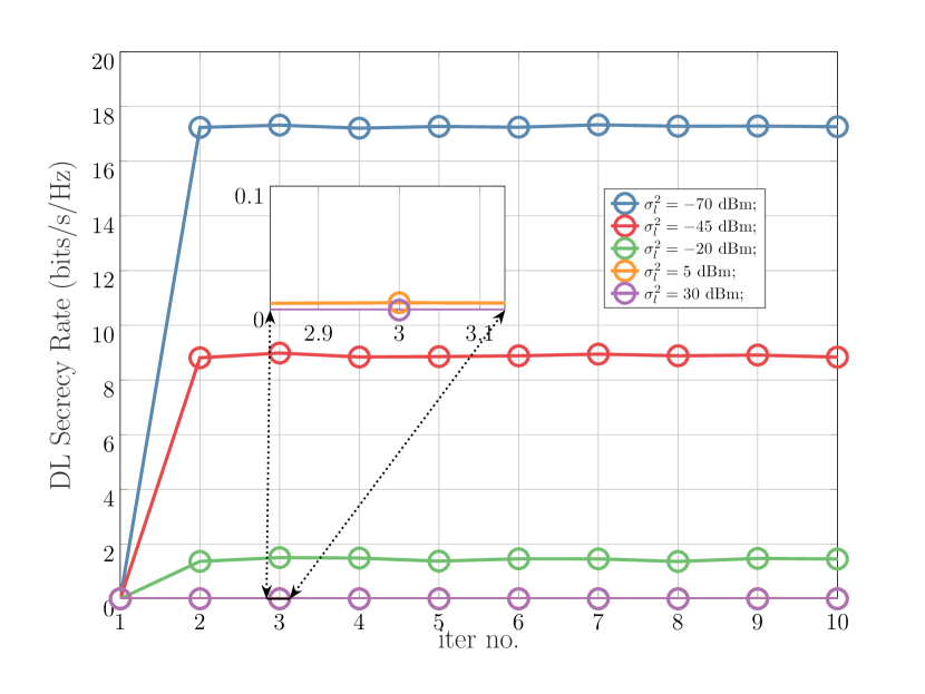
In Fig. 4, we set the same simulation parameters as Fig. 2 except for , , and . We study the impact of on the DL sum secrecy rate with increasing iteration number. The more noisy a DL user, the less of a DL sum secrecy rate the algorithm settles at. For instance, for a , the DL sum secrecy rate converges to as opposed to at . When the noise variance exceeds , which is already too high, the DL sum secrecy rate is near-zero. This is because at a fixed power budget and ISMR level, the DL noise variance can only decrease the DL sum secrecy rate, which is an intuitive observation. We also observe, as in Fig. 2 and Fig. 3, that the algorithm converges in all cases.

In Fig. 5, we set the same simulation parameters as Fig. 4 except for antennas and . We study the impact of both number of DFRC BS receive antennas, i.e. , and the noise variance at DFRC BS, i.e. , on the convergence behavior of the UL sum secrecy rate. For any , we see that increasing the number of receive antennas can improve the DL sum secrecy rate for fixed power budget, and fixed ISMR levels. For instance, at fixed , we see that with antennas, the IJTB algorithm converges to an UL sum secrecy rate of about , as compared to for antennas, and for antennas. This is because DFRC receive antennas can also allow room for enhanced degrees-of-freedom which enables better UL sum secrecy rate for the algorithm to converge towards. We observe that the algorithm needs about iterations to converge to a stable point.

In Fig. 6, we set the same simulation parameters as Fig. 2 except for the following: antennas, user, evesdroppers, , , and . We study the performance of the IJTB method from an UL sum secrecy rate sense with increasing UL radial distance and for different eavesdropper distances. It is evident that with increasing , the UL decreases regardless of the method. However, it is worthwhile noting that the IJTB method dominates all other benchmarks regardless of and . Even more, the IJTB method can adapt to different , which is not a common feature with the other benchmark. For instance, the UL sum secrecy rate of all benchmarks drops to a low near-zero rate when the eavesdropper reaches a distance of .

In Fig. 7, we fix the same simulation parameters as that of Fig. 6. Furthermore, we analyze the efficacy of the IJTB approach in terms of overall sum secrecy rate as the UL user distance increases, considering various distances of potential eavesdroppers. We observe that the sum secrecy rate decreases with UL sum secrecy rate for all methods. In addition, a far eavesdropper would normally contribute to an increase in sum secrecy rate. This is because of increased pathloss. What’s interesting to observe is that for a close eavesdropper (i.e. ), the impact of AN is more effective, which is seen by the two isotropic benchmarks (isotropic and non-isotropic benchmarks), where there is about gap in favor of the isotropic AN benchmark. However, when the eavesdropper distance becomes high (i.e. ), the impact of AN is no longer effective. It is also interesting to observe that any random solution of power vector, beamformers and AN beamforming on average keeps the sum secrecy rate at zero. On the other hand, the IJTB method can adapt to eavesdropper distance changes as can be seen because both curves corresponding to the IJTB method at the two different eavesdropper distances coincide. Even more, the IJTB method outperforms all other methods in terms of sum secrecy rate over all the evaluated UL user distances. For instance, when , the IJTB method achieves a sum secrecy rate of about as opposed achieved by the isotropic no-AN benchmark.

In Fig. 8, we fix the same simulation parameters as Fig. 2 except for eavesdropper, , and . We study the sum secrecy rate vs. ISMR ISAC trade-off for different channel conditions. When the ISMR constraint imposes a stringent restriction through a tight (low) the sum secrecy rate of the IJTB method drops lower than the isotropic benchmarking methods. This is because the IJTB method is basically dedicating an optimized chunk of power towards the eavesdropper through the mainlobes, while restricting power onto the sidelobes. However, it is interesting to see that the IJTB method is still able to achieve high sum secrecy rates, which are, in some channel conditions, comparable with the benchmarks. For example, in Rayleigh channel conditions () and at a tight ISMR corresponding to , the sum secrecy rate is about and as the ISMR constraint becomes less and less stringent (i.e. increasing ), the sum secrecy rate of the IJTB method gradually increases to increase the maximum possible sum secrecy rate the ISAC system can achieve. For example, the sum secrecy rate reaches and at high for Rayleigh and strong LoS channel conditions, respectively. This is because the channel conditions hold significant amount of information regarding the sum secrecy rate of the IJTB system. Clearly, the sum secrecy rates of all other benchmarks do not depend on the because they are not optimized for good ISMR performance.

In Fig. 9, we set the same simulation parameters as Fig. 2 except for and . Moreover, we analyze the impact of the on the achieved ISMR of the IJTB method. We can see a clear trend between the obtained ISMR and the tuned one via . Notice that the evaluated ISMR is always upper bounded by the given , which tells us that this constraint is always active. Interestingly, as increases, the ISMR tries to hold on to a tighter value. For example, for eavesdroppers, when we set an of , the achieved ISMR is , as opposed to for eavesdroppers and for eavesdroppers. Also, when , we see that the case of eavesdroppers saturates at about . This is because more energy has to be contained within the mainlobes, as compared to the sidelobes, towards the different target eavesdroppers.
VI Conclusion
This paper examines an FD-ISAC system with multiple malicious targets aiming to intercept UL and DL communications and provides an ISAC optimization framework for optimizing the UL and DL sum secrecy rate under sensing and power budget constraints. This enables one quantifying the maximum achievable FD secrecy rates, under ISAC constraints. Furthermore, we introduced IJBT, a method well-suited for the proposed FD-ISAC sum secrecy rate maximization problem at hand, which alternates between sub-problems to efficiently solve for beamformers and power allocations. Our results support the effectiveness of the method, as compared to benchmarking techniques. In conclusion, our findings demonstrate that the IJTB algorithm not only exhibits rapid convergence, but also consistently outperforms other methods by maintaining higher sum secrecy rates, even as the eavesdropper distance increases. Furthermore, IJTB maintains strong performance, particularly as the ISMR constraint becomes less stringent, highlighting its robustness in securing SAC applications.
Appendix A Proof of Lemma 1
The Taylor series expansion of around can be expressed as \useshortskip
| (42) | ||||
The partial derivatives are trivial to calculate since every term appearing in is linear. This can be easily rearranged as follows \useshortskip
| (43) | ||||
leading to equation (23).
Appendix B Acknowledgment
This work has been supported by Tamkeen and the Center for Cybersecurity under the NYU Abu Dhabi Research Institute Award G1104.
References
- [1] M. A. Richards, J. Scheer, W. A. Holm, and W. L. Melvin, “Principles of modern radar,” 2010.
- [2] S. Naoumi, A. Bazzi, R. Bomfin, and M. Chafii, “Complex Neural Network based Joint AoA and AoD Estimation for Bistatic ISAC,” IEEE Journal of Selected Topics in Signal Processing, pp. 1–15, 2024.
- [3] A. Chowdary, A. Bazzi, and M. Chafii, “On Hybrid Radar Fusion for Integrated Sensing and Communication,” IEEE Transactions on Wireless Communications, vol. 23, no. 8, pp. 8984–9000, 2024.
- [4] A. Liu, Z. Huang, M. Li, Y. Wan, W. Li, T. X. Han, C. Liu, R. Du, D. K. P. Tan, J. Lu, Y. Shen, F. Colone, and K. Chetty, “A Survey on Fundamental Limits of Integrated Sensing and Communication,” IEEE Communications Surveys & Tutorials, vol. 24, no. 2, pp. 994–1034, 2022.
- [5] Z. Behdad, O. T. Demir, K. W. Sung, E. Björnson, and C. Cavdar, “Multi-Static Target Detection and Power Allocation for Integrated Sensing and Communication in Cell-Free Massive MIMO,” IEEE Transactions on Wireless Communications, pp. 1–1, 2024.
- [6] N. Xue, X. Mu, Y. Liu, and Y. Chen, “NOMA Assisted Full Space STAR-RIS-ISAC,” IEEE Transactions on Wireless Communications, pp. 1–1, 2024.
- [7] B. Smida, R. Wichman, K. E. Kolodziej, H. A. Suraweera, T. Riihonen, and A. Sabharwal, “In-band full-duplex: The physical layer,” Proceedings of the IEEE, pp. 1–30, 2024.
- [8] A. Bazzi and M. Chafii, “On Integrated Sensing and Communication Waveforms With Tunable PAPR,” IEEE Transactions on Wireless Communications, vol. 22, no. 11, pp. 7345–7360, 2023.
- [9] M. Chafii, L. Bariah, S. Muhaidat, and M. Debbah, “Twelve scientific challenges for 6g: Rethinking the foundations of communications theory,” IEEE Communications Surveys & Tutorials, vol. 25, no. 2, pp. 868–904, 2023.
- [10] A. Bazzi and M. Chafii, “Secure Full Duplex Integrated Sensing and Communications,” IEEE Transactions on Information Forensics and Security, vol. 19, pp. 2082–2097, 2024.
- [11] A. Chorti, A. N. Barreto, S. Köpsell, M. Zoli, M. Chafii, P. Sehier, G. Fettweis, and H. V. Poor, “Context-aware security for 6g wireless: The role of physical layer security,” IEEE Communications Standards Magazine, vol. 6, no. 1, pp. 102–108, 2022.
- [12] “New SID on Security Aspects of Integrated Sensing and Communication,” 3GPPSA3-e(AH) for Rel-19 SID/WID workshop, S3-23xxxx, eMeeting, 27-28 September 2023. Revision of S3ah-230038+230055+230068, 2023, document for Approval, Agenda Item: 4. [Online]. Available: http://www.3gpp.org/Work-Items
- [13] D. Xu, X. Yu, D. W. K. Ng, A. Schmeink, and R. Schober, “Robust and secure resource allocation for isac systems: A novel optimization framework for variable-length snapshots,” IEEE Transactions on Communications, vol. 70, no. 12, pp. 8196–8214, 2022.
- [14] Z. Ren, L. Qiu, J. Xu, and D. W. K. Ng, “Robust transmit beamforming for secure integrated sensing and communication,” IEEE Transactions on Communications, vol. 71, no. 9, pp. 5549–5564, 2023.
- [15] N. Su, F. Liu, and C. Masouros, “Sensing-assisted eavesdropper estimation: An isac breakthrough in physical layer security,” IEEE Transactions on Wireless Communications, vol. 23, no. 4, pp. 3162–3174, 2024.
- [16] P. Liu, Z. Fei, X. Wang, B. Li, Y. Huang, and Z. Zhang, “Outage constrained robust secure beamforming in integrated sensing and communication systems,” IEEE Wireless Communications Letters, vol. 11, no. 11, pp. 2260–2264, 2022.
- [17] A. A. Nasir, “Joint Users’ Secrecy Rate and Target’s Sensing SNR Maximization for a Secure Cell-Free ISAC System,” IEEE Communications Letters, vol. 28, no. 7, pp. 1549–1553, 2024.
- [18] A. Bazzi and M. Chafii, “On Outage-Based Beamforming Design for Dual-Functional Radar-Communication 6G Systems,” IEEE Transactions on Wireless Communications, vol. 22, no. 8, pp. 5598–5612, 2023.
- [19] M. Mohammadi, Z. Mobini, D. Galappaththige, and C. Tellambura, “A comprehensive survey on full-duplex communication: Current solutions, future trends, and open issues,” IEEE Communications Surveys & Tutorials, vol. 25, no. 4, pp. 2190–2244, 2023.
- [20] Z. Xiao and Y. Zeng, “Waveform design and performance analysis for full-duplex integrated sensing and communication,” IEEE Journal on Selected Areas in Communications, vol. 40, no. 6, pp. 1823–1837, 2022.
- [21] Z. He, W. Xu, H. Shen, D. W. K. Ng, Y. C. Eldar, and X. You, “Full-duplex communication for isac: Joint beamforming and power optimization,” IEEE Journal on Selected Areas in Communications, vol. 41, no. 9, pp. 2920–2936, 2023.
- [22] Y. Guo, Y. Liu, Q. Wu, X. Li, and Q. Shi, “Joint beamforming and power allocation for ris aided full-duplex integrated sensing and uplink communication system,” IEEE Transactions on Wireless Communications, vol. 23, no. 5, pp. 4627–4642, 2024.
- [23] Z. Liu, S. Aditya, H. Li, and B. Clerckx, “Joint transmit and receive beamforming design in full-duplex integrated sensing and communications,” IEEE Journal on Selected Areas in Communications, vol. 41, no. 9, pp. 2907–2919, 2023.
- [24] D. Galappaththige, C. Tellambura, and A. Maaref, “Integrated sensing and backscatter communication,” IEEE Wireless Communications Letters, vol. 12, no. 12, pp. 2043–2047, 2023.
- [25] C. B. Barneto, S. D. Liyanaarachchi, M. Heino, T. Riihonen, and M. Valkama, “Full duplex radio/radar technology: The enabler for advanced joint communication and sensing,” IEEE Wireless Communications, vol. 28, no. 1, pp. 82–88, 2021.
- [26] R. Allu, M. Katwe, K. Singh, T. Q. Duong, and C.-P. Li, “Robust Energy Efficient Beamforming Design for ISAC Full-Duplex Communication Systems,” IEEE Wireless Communications Letters, pp. 1–1, 2024.
- [27] D. Galappaththige, S. Zargari, C. Tellambura, and G. Y. Li, “Near-Field ISAC: Beamforming for Multi-Target Detection,” IEEE Wireless Communications Letters, pp. 1–1, 2024.
- [28] C. Jiang, C. Zhang, C. Huang, J. Ge, J. He, and C. Yuen, “Secure beamforming design for ris-assisted integrated sensing and communication systems,” IEEE Wireless Communications Letters, vol. 13, no. 2, pp. 520–524, 2024.
- [29] H. Zhao, F. Wu, W. Xia, Y. Zhang, Y. Ni, and H. Zhu, “Joint beamforming design for ris-aided secure integrated sensing and communication systems,” IEEE Communications Letters, vol. 27, no. 11, pp. 2943–2947, 2023.
- [30] F. Xia, Z. Fei, X. Wang, P. Liu, J. Guo, and Q. Wu, “Joint Waveform and Reflection Design for Sensing-Assisted Secure RIS-Based Backscatter Communication,” IEEE Wireless Communications Letters, vol. 13, no. 5, pp. 1523–1527, 2024.
- [31] G. Sun, H. Shi, B. Shang, and W. Hao, “Secure transmission for active ris-assisted thz isac systems with delay alignment modulation,” IEEE Communications Letters, vol. 28, no. 5, pp. 1019–1023, 2024.
- [32] J. Zhang, J. Xu, W. Lu, N. Zhao, X. Wang, and D. Niyato, “Secure Transmission for IRS-Aided UAV-ISAC Networks,” IEEE Transactions on Wireless Communications, pp. 1–1, 2024.
- [33] Y. Liu, I. Al-Nahhal, O. A. Dobre, F. Wang, and H. Shin, “Extreme Learning Machine-Based Channel Estimation in IRS-Assisted Multi-User ISAC System,” IEEE Transactions on Communications, vol. 71, no. 12, pp. 6993–7007, 2023.
- [34] R. W. Heath, N. González-Prelcic, S. Rangan, W. Roh, and A. M. Sayeed, “An Overview of Signal Processing Techniques for Millimeter Wave MIMO Systems,” IEEE Journal of Selected Topics in Signal Processing, vol. 10, no. 3, pp. 436–453, 2016.
- [35] F. Liu, Y. Cui, C. Masouros, J. Xu, T. X. Han, Y. C. Eldar, and S. Buzzi, “Integrated Sensing and Communications: Toward Dual-Functional Wireless Networks for 6G and Beyond,” IEEE Journal on Selected Areas in Communications, vol. 40, no. 6, pp. 1728–1767, 2022.
- [36] P. Zhao, M. Zhang, H. Yu, H. Luo, and W. Chen, “Robust Beamforming Design for Sum Secrecy Rate Optimization in MU-MISO Networks,” IEEE Transactions on Information Forensics and Security, vol. 10, no. 9, pp. 1812–1823, 2015.
- [37] B. Ma, H. Shah-Mansouri, and V. W. S. Wong, “Full-Duplex Relaying for D2D Communication in Millimeter Wave-based 5G Networks,” IEEE Transactions on Wireless Communications, vol. 17, no. 7, pp. 4417–4431, 2018.
- [38] I. A. Hemadeh, K. Satyanarayana, M. El-Hajjar, and L. Hanzo, “Millimeter-Wave Communications: Physical Channel Models, Design Considerations, Antenna Constructions, and Link-Budget,” IEEE Communications Surveys & Tutorials, vol. 20, no. 2, pp. 870–913, 2018.
- [39] A. Sabharwal, P. Schniter, D. Guo, D. W. Bliss, S. Rangarajan, and R. Wichman, “In-Band Full-Duplex Wireless: Challenges and Opportunities,” IEEE Journal on Selected Areas in Communications, vol. 32, no. 9, pp. 1637–1652, 2014.
- [40] A. T. Le, X. Huang, and Y. J. Guo, “A Two-Stage Analog Self-Interference Cancelation Structure for High Transmit Power In-Band Full-Duplex Radios,” IEEE Wireless Communications Letters, vol. 11, no. 11, pp. 2425–2429, 2022.
- [41] Y. Zhang, J. Mu, and J. Xiaojun, “Performance of Multi-Cell mmWave NOMA Networks With Base Station Cooperation,” IEEE Communications Letters, vol. 25, no. 2, pp. 442–445, 2021.
- [42] B. Hassibi and T. Marzetta, “Multiple-antennas and isotropically random unitary inputs: the received signal density in closed form,” IEEE Transactions on Information Theory, vol. 48, no. 6, pp. 1473–1484, 2002.
- [43] A. Waraiet, K. Cumanan, Z. Ding, and O. A. Dobre, “Deep Reinforcement Learning-Based Robust Design for an IRS-Assisted MISO-NOMA System,” IEEE Transactions on Machine Learning in Communications and Networking, vol. 2, pp. 424–441, 2024.
- [44] Y. Ju, Y. Chen, Z. Cao, L. Liu, Q. Pei, M. Xiao, K. Ota, M. Dong, and V. C. M. Leung, “Joint Secure Offloading and Resource Allocation for Vehicular Edge Computing Network: A Multi-Agent Deep Reinforcement Learning Approach,” IEEE Transactions on Intelligent Transportation Systems, vol. 24, no. 5, pp. 5555–5569, 2023.