Successive finite element methods for Stokes equations
Abstract
This paper will suggest a new finite element method to find a -velocity and a -pressure solving Stokes equations. The method solves first the decoupled equation for the -velocity. Then, four kinds of local -pressures and one -pressure will be calculated in a successive way. If we superpose them, the resulting -pressure shows the optimal order of convergence same as a -projection. The chief time cost of the new method is on solving two linear systems for the -velocity and -pressure, respectively.
1 Introduction
High order finite element methods for incompressible Stokes problems have been developed well in 2-dimensional domain and analyzed along to the inf-sup condition [5, 7, 10]. They, however, endure their large numbers of degrees of freedom. To be worse in case of Scott-Vogelius, instability appears on pressure, if the mesh bears singular vertices.
Recently, we found a so called sting function having an interesting quadrature rule. In the Scott-Vogelius finite element method, it causes the discrete Stokes problem to be singular on the presence of exactly singular vertices. Even on nearly singular vertices, the pressure solution is easy to be spoiled. To overcome the problem based on understanding the causes, we did a new error analysis in a successive way and restored the ruined pressure by simple post-process driven from it [9].
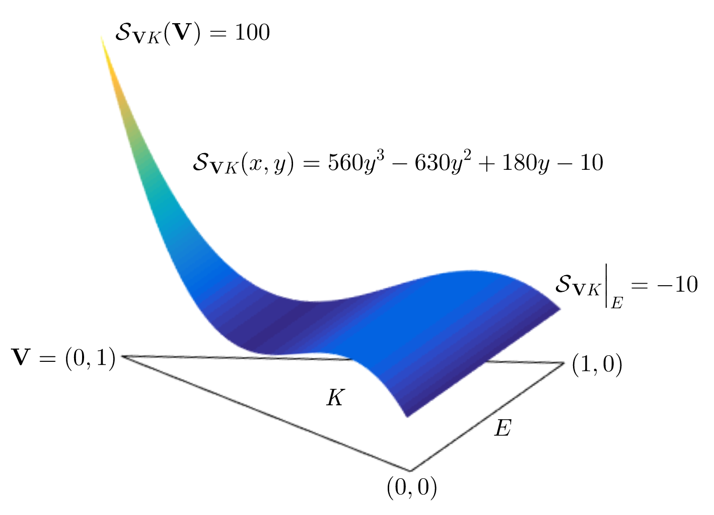
In this paper, we will suggest a new finite element method to calculate a pressure solution at low cost, utilizing the successive way in the precedented new error analysis. In our method, the characteristics of a sting function depicted in Figure 1 will also play a key role.
We will solve first the decoupled equation for velocity in the divergence-free space inherited from the -Argyris stream function space. It is simpler and smaller than the divergence-free subspace of the - Scott-Vogelius finite element space.
The main stage of our method is the successive 5 steps calculating four kinds of local -pressures for triangles, regular vertices, nearly singular vertices and singular corners, respectively, as well as one -pressure in the last step. They are successive in the sense that each step needs the calculated in the previous step.
Superposition of all the calculated reaches at the final -pressure which shows the optimal order of convergence same as a -projection of the continuous pressure. The chief time cost of the new method is on solving two linear systems for the -velocity and -pressure, respectively.
The paper is organized as follows. In the next section, the detail on finding a -velocity will be offered. After short review of nearly singular vertices in Section 3, we will introduce a new basis for -pressures consisting of non-sting, sting and constant functions and decompose the space of -pressures in Section 4. Then, we will devote Section 5 to describing the successive 5 steps to find a -pressure solution. Finally, a numerical test will be presented in the last section.
Throughout the paper, for a set , standard notations for Sobolev spaces are employed and is the space of all whose integrals over vanish. We will use , and for the norm, seminorm for and inner product, respectively. If , it may be omitted in the indices. Denoting by , the space of all polynomials on of order less than or equal , will mean that coincides with a polynomial in on .
2 Velocity from the decoupled equation
Let be a simply connected polygonal domain in and a regular family of triangulations of . Denote by , discrete polynomial spaces:
In this paper, we will approximate a pair of velocity and pressure which satisfies an incompressible Stokes problem:
| (1) |
for a given body force .
Defining a divergence-free space as
we can solve satisfying
| (2) |
Theorem 2.1.
Let satisfy (1). If , then
| (3) |
3 Nearly singular vertex
A vertex is called exactly singular if the union of all edges sharing belongs to the union of two lines. To be precise, let be all triangles sharing and denote by , the angle of at , . Define
Then if and only if is exactly singular.
Since is regular, there exists such that
which depends on the shape regularity parameter of . Set
then call a vertex to be nearly singular if or
otherwise regular. From the following lemma [9], we note that each interior nearly singular vertex is isolated from others.
Lemma 3.1.
There is no interior edge connecting two nearly singular vertices.
4 Decomposition of
For each triangle , define
In the remaining of the paper, we will use the following notations:
-
: a generic constant which depends only the shape regularity parameter of ,
-
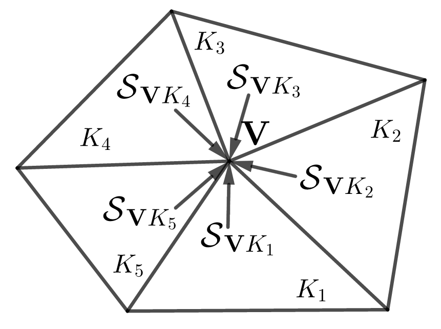
: the union of all triangles in sharing a vertex as in Figure 3-(b),
-
: the set of all vertices in ,
-
: the area and length of a triangle and an edge , respectively.
4.1 sting function
Let be a vertex of a triangle . Then there exists a unique function satisfying the following quadrature rule:
| (6) |
since the both sides of (6) are linear functionals on . We call a sting function of on , named after the shape of its graph as in Figure 1.
In the reference triangle of vertices , we have the following 3 sting functions:
| (7) |
Since for an affine transformation , we estimate
| (8) |
4.2 non-sting function
Given triangle of vertices , the following 16-point Lyness quadrature rule is exact for every polynomial :
| (9) |
where belong to and is the gravity center of and are the centers of the medians, that is,
Lemma 4.1.
If a cubic function satisfies the following 10 conditions, then .
| (10) |
Proof.
Since is the gravity center of , it suffices to prove in case
Let
From the condition (10), vanishes on the line and . It means
| (11) |
Then since , we deduce
| (12) |
Similarly, from , we have
| (13) |
We note that since . Thus, we can write
| (14) |
From the unisolvancy in the above lemma, for each , we can define two functions , called non-sting, by their following values:
| (15) |
where is the Kronecker delta.
In the reference triangle of vertices , they appear in
We note that
| (16) |
4.3 basis for
Given triangle of vertices and centers of medians, define a set
Lemma 4.2.
is a basis for
4.4 decomposition of
Given triangle , let be a space spanned by 6 non-sting functions in , that is,
Then by Lemma 4.2, we can decompose into
| (21) |
Given vertex , let be a space spanned by all sting functions of , that is,
where are all triangles in sharing .
We call a sting pressure of and a non-sting pressure of . Examples of their supports are depicted in Figure 2.
is determined by

is determined by
Then from (21), we can decompose into
| (22) |
5 Successive method for pressure
In this section, we will find the following discrete pressures:
in a successive way consisting of the following 5 steps.
- Step 1.
-
Calculate a non-sting pressure using for each triangle and superpose them to form
- Step 2.
-
Calculate a sting pressure using for each regular vertex and superpose them to form
- Step 3.
-
Calculate a sting pressure using for each nearly singular vertex except corners and superpose them to form
- Step 4.
-
Calculate a sting pressure using for each nearly singular corner and superpose them to form
- Step 5.
-
Calculate a piecewise constant pressure using .
The detail of Step above will be given in Section 5. below, .
If we define as
| (23) |
it shows the optimal order of convergence as in the following theorem.
Theorem 5.1.
Let satisfy (1). If , then
| (24) |
5.0 decomposition of
Let be a Hermite interpolation of in the theorem 5.1 such that
| (25) |
at all vertices and gravity centers of triangles in . Then from (22), we can split into
| (26) |
where
| (27) |
We note that satisfies that
| (28) |
We assume the following to exclude pathological meshes.
Assumption 5.1.
has no two adjacent triangles whose union has two corner points of .
5.1 Step 1. non-sting pressure for triangle
Let’s fix a triangle of vertices and centers of medians. There exists a unique function such that
Then by same argument as in (19) with a test function , all 6 non-sting basis functions of satisfy
| (29) |
Generally, for each , choose such that
| (30) |
and define
| (31) |
Then by same argument as in (29) with (15), (30), (31), all 6 basis functions of satisfy
| (32) |
Now with the aid of (32), we can find a unique such that
| (33) |
Actually, if we set for 6 unknown constants as
we deduce that
| (34) |
Lemma 5.2.
| (35) |
Proof.
Superpose all the calculated non-sting pressures and define
| (40) |
5.2 Step 2. sting pressure for regular vertex
5.2.1 test functions in two triangles
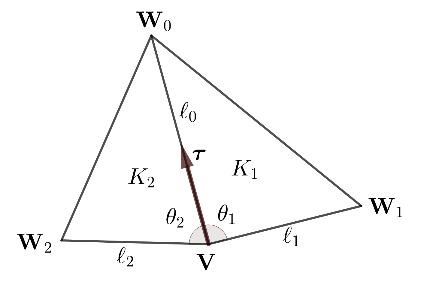
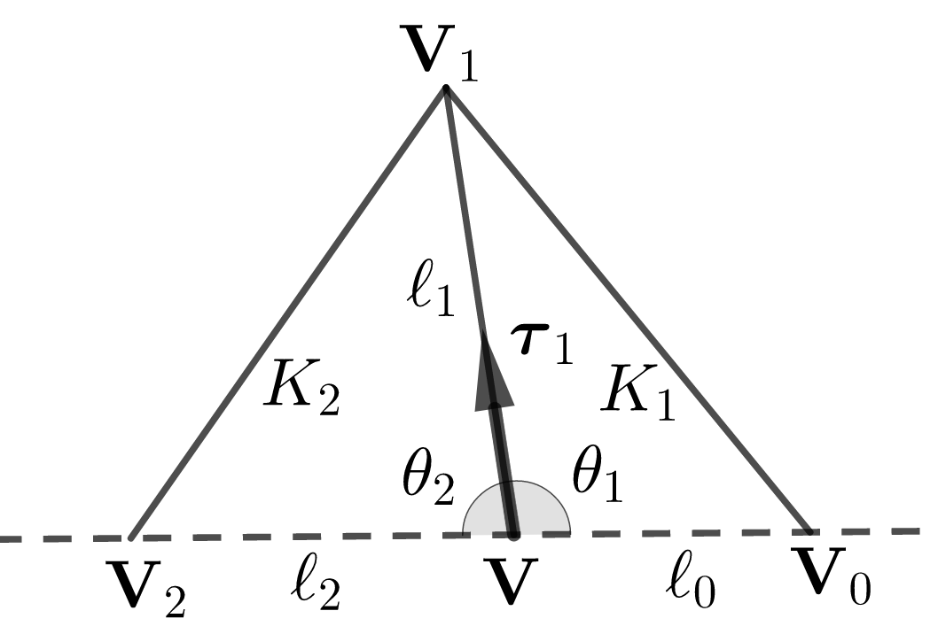
Let be a vertex and two back-to-back triangles sharing as in Figure 3-(a). Denote by , other 3 vertices and a unit tangent vector such that
There exists a function such that
| (41) |
Assume are counterclockwisely numbered with respect to . Then by simple calculation, we have
| (42) |
where denotes the counterclockwise rotation of vector . Thus if we set a test function for a vector , it satisfies
| (43) |
and vanishes at all other vertices.
Let be represented with some constants as
that is, it is a sum of sting pressures on . Then, by quadrature rule of sting functions in (6), we expand from (43) that
It can be written in simpler form:
| (44) |
where are angles of at , respectively, and as in Figure 3-(a).
5.2.2 least square solution
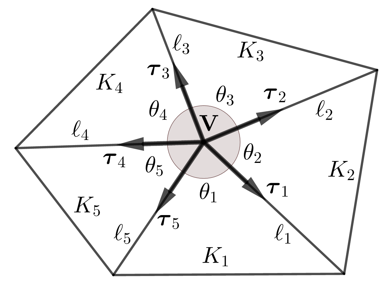
Let’s fix an interior vertex and all triangles in sharing as in Figure 3-(b). We assume the numbering is counterclockwise and use the index modulo .
For each , name a vertex and a unit tangent vector so that
| (45) |
There exists a function such that
| (46) |
for each . For the uniqueness of , we add the following condition:
| (47) |
Then we prepare test functions in as
| (48) |
Let , a sum of sting pressures of , be represented as
| (49) |
with unknown constants . Consider the following system of equations:
| (50a) | |||
| (50b) | |||
for .
Lemma 5.3.
If is a regular vertex, then the smallest singular value of the system in (50) satisfies
| (51) |
Proof.
Let be an angle of at and as in Figure 3-(b). Then from (44), (46), (49), we can rewrite (50) as, for ,
| (52a) | ||||
| (52b) | ||||
We note that the sting component of in (26) and in (46) satisfies
| (56) |
since and vanishes at all vertices except .
Let be the least square solution of the system (50). Then the error is estimated in the following lemma.
Lemma 5.4.
Let be a regular vertex. Then, the least square solution of (50) satisfies
| (57) |
Proof.
Even in case of regular vertices on , we can copy the above argument to establish Lemma 5.3 and 5.4 with a system of equations.
Denote by , the superposition of all the calculated pressures up to now, that is,
| (60) |
where is a set of all regular vertices.
5.3 Step 3. sting pressure for nearly singular vertex except corners
When a vertex is exactly singular, the system (50) is underdetermined, since the determinant of (53) makes
Although is not exactly singular, the error in (59) goes through a tiny smallest singular value, if it is nearly singular.
To overcome the problem on nearly singular vertices, we will replace equations in (50b) with new equations utilizing jumps of in (60) we have already calculated.
5.3.1 boundary singular vertex not a corner
Let’s fix a boundary vertex which is not a corner point of . If is nearly singular, it is exact and has only two triangle which share as in Figure 4-(a). Denote by , other 3 vertices and a unit tangent vector such that
Define the jump of a function across at as
| (61) |
If is nearly singular, then instead of (50b), consider the following new system of equations:
| (62a) | ||||
| (62b) | ||||
Lemma 5.5.
Let be a boundary nearly singular vertex, not a corner of . If is the solution of (62), then we estimate
| (63) |
Proof.
Since is continuous on , we have . It is written in
| (64) |
Thus, if we denote the error by , by same argument in regular case, we get
|
|
(65) |
We can represent with unknown constants as
| (66) |
Let be angles of at , respectively, and as in Figure 4-(a). Then, from the property of sting functions in (7), we have
| (67) |
If the first right hand side in (65) is abbreviated by , we can rewrite (65) into
| (68) |
We can repeat the same in regular case for the estimation:
| (69) |
If we have the following similar estimation for the second right hand side in (68):
|
|
(70) |
the estimation (63) will be established from (8), (66)-(70).
If is an interior vertex, it is regular by Lemma 3.1. Even in case of a boundary vertex , it is regular unless . We exclude that pathological case by Assumption 5.1. Thus, we conclude that is a regular vertex.
We also note that , are constant on from (7). It means that they do not have any effect on and . It results in
| (71) |
Similarly, whether are regular or not, we have
| (72) |
| (73) |
5.3.2 interior singular vertex
Let be an interior vertex and go back to the setting in Section 5.2.2 as in Figure 3-(b). For each , define the jump of a function across at as
| (75) |
If is nearly singular, replace (50b) with new equations using the jumps of in (75). That is, we consider the following system of equations:
| (76a) | ||||
| (76b) | ||||
Let be the least square solution of (76). We note that all other adjacent vertices are regular from Lemma 3.1. Thus we can repeat the arguments in the proofs of Lemma 5.3, 5.4, 5.5 to establish the following lemma.
Lemma 5.6.
Let be an interior nearly singular vertex. If be the least square solution of (76), then we estimate
| (77) |
Denote by , the superposition of all the calculated pressures up to now, that is,
| (78) |
where is a set of all vertices except nearly singular corner points of .
5.4 Step 4. sting pressure for nearly singular corner
Let be a corner point of which is nearly singular and , triangles in sharing . If , we can calculate the least square solution satisfying the system of equations as in (76) and estimate its error as in (77).
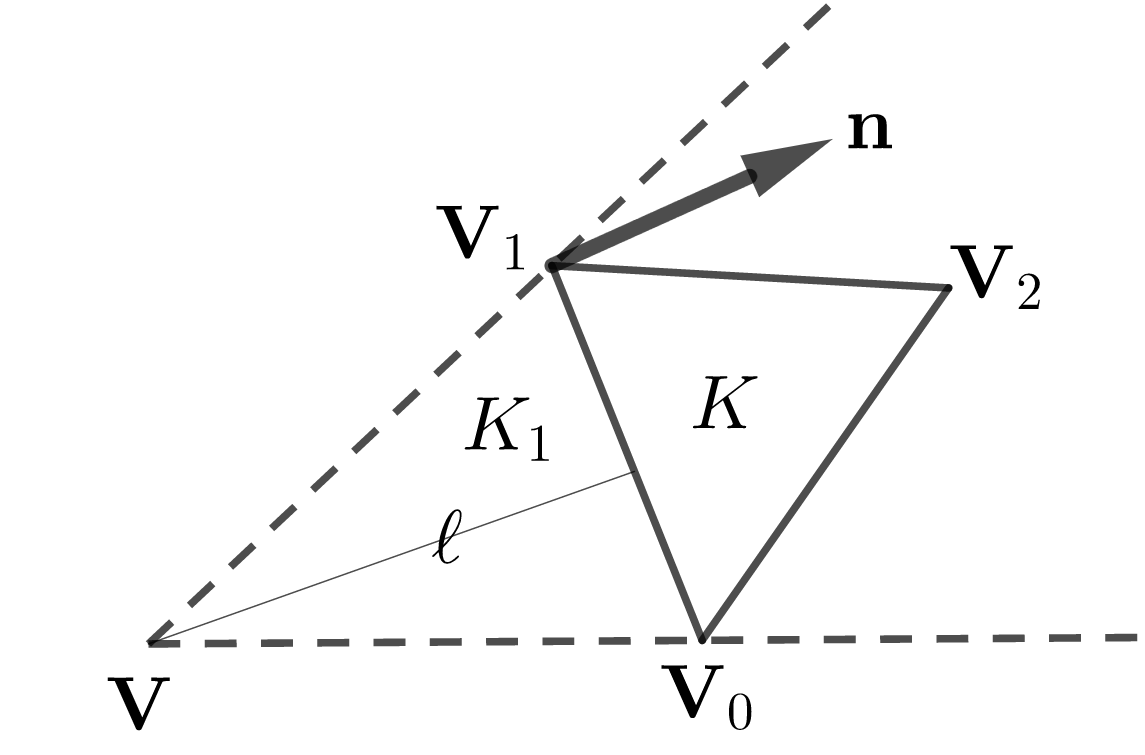
If , there exists a triangle in sharing two vertices with as in Figure 4-(b). Denote by , the third vertex of not shared with .
Define the jump of a function across at as
| (79) |
where is a unit outward normal vector on of and is the distance between and . Then we can determine for some constant satisfying
| (80) |
Lemma 5.7.
Let be a corner which meets only one triangle. If is the solution of (80), then we estimate
| (81) |
Proof.
We note that is continuous at , since it is a Hermite interpolation of in (25). It can be written in
| (82) |
Set the error for some constant , then from (80), (82), we have
| (83) |
From the property of sting functions in (7), we have
| (84) |
We have already calculated , , since are not corners by Assumption 5.1. Thus the difference in (83) is written as
| (85) |
Denote by , the superposition of all the calculated pressures up to now,
| (87) |
where is a set of all vertices in . For notation consistency, denote again
| (88) |
Then hereby, we have established the following lemma.
Lemma 5.8.
5.5 Step 5. piecewise constant pressure
Let be a space of all functions in vanishing at all vertices and whose value at the midpoint of each edge is normal to . Define
Then, there exists a unique which satisfies a following discrete Stokes problem:
| (89) |
Denote by , the average of a function over , then define
| (90) |
Lemma 5.9.
| (91) |
Proof.
Then, we can rewrite (89) for all ,
| (94) |
Denote the error by . Then from (92), (94), we have for all ,
| (95) |
Since , there exists a nonzero such that
| (96) |
from the inf-sup condition, where is a constant, independent of .
6 Numerical test
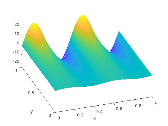
We tested the suggested successive method in with the velocity and pressure such that
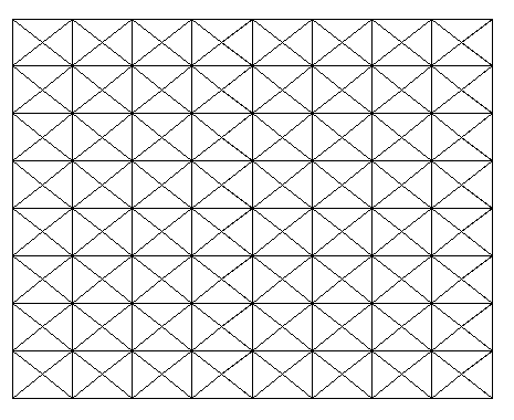
For triangulations, we first formed the meshes of uniform squares over , then added one exactly singular vertex in every square. An example of mesh is given in Figure 5.
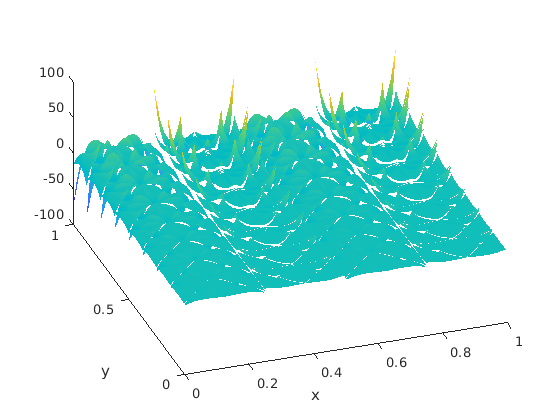
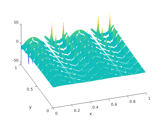
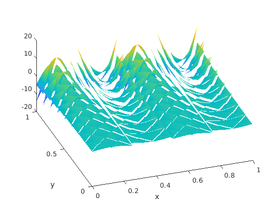
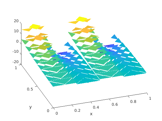
We have calculated the successive pressures and along to Step 1,2,3,5 in Section 5. Since the meshes have not any singular corner, . Their examples are depicted in Figure 6 as well as .
The error table in Table 1 shows the optimal order of convergence, expected in Theorem 2.1 and 5.1. We adopted a direct linear solver in LAPACK on solving the systems from the problem (2) and (89) to focus on testing the suggested method.
| mesh | order | order | ||
|---|---|---|---|---|
| 4 x 4 x 4 | 1.1264E-2 | 5.8000E-2 | ||
| 8 x 8 x 4 | 6.1498E-4 | 4.1950 | 2.7012E-3 | 4.4244 |
| 16 x 16 x 4 | 3.5942E-5 | 4.0968 | 1.6760E-4 | 4.0105 |
| 32 x 32 x 4 | 2.2002E-6 | 4.0299 | 1.0454E-5 | 4.0029 |
References
- [1] C. Bernardi and G. Raugel, Analysis of some finite elements for the Stokes problem, Mathematics of Computation, 44 (1985), 71-79, DOI: 10.2307/2007793
- [2] S. C. Brenner and L. R. Scott, The mathematical theory of finite element methods, Springer-Verlag, New York, 2nd edition, 2002
- [3] F. Brezzi and M. Fortin, Mixed and hybrid finite element methods, Springer-Verlag, New York, 1991
- [4] P. G. Ciarlet, The finite element method for elliptic equations, North-Holland, Amsterdam, 1978
- [5] R. S. Falk and M. Neilan, Stokes complexes and the construction of stable finite elements with pointwise mass conservation, SIAM journal of Numerical Analysis, 51 (2013), 1308-1326, DOI: 10.1137/120888132
- [6] V. Girault and P. A. Raviart, Finite element methods for the Navier-Stokes equations: Theory and Algorithms, Springer-Verlag, New York, 1986
- [7] J. Guzman and L. R. Scott, The Scott-Vogelius finite elements revisited, Mathematics of Computation, electronically published (2018), DOI: 10.1090/mcom/3346
- [8] J. N. Lyness and D. Jespersen, Moderate degree symmetric quadrature rules for the triangle, IMA Journal of Applied Mathematics, 15 (1975), 19-32, DOI: 10.1093/imamat/15.1.19
- [9] C. Park, Spurious pressure in Scott–Vogelius elements, Journal of Computational and Applied Mathematics, 363 (2020), 370-391, https://doi.org/10.1016/j.cam.2019.06.007
- [10] L. R. Scott and M. Vogelius, Norm estimates for a maximal right inverse of the divergence operator in spaces of piecewise polynomials, ESIAM: M2AN, 19 (1985), 111-143, DOI: 10.1051/m2an/1985190101111