Subwavelength Su-Schrieffer-Heeger topological modes in acoustic waveguides
Abstract
Topological systems furnish a powerful way of localizing wave energy at edges of a structured material. Usually this relies on Bragg scattering to obtain bandgaps with nontrivial topological structures. However, this limits their applicability to low frequencies since that would require very large structures. A standard approach to address the problem is to add resonating elements inside the material to open gaps in the subwavelength regime. Unfortunately, one usually has no precise control on the properties of the obtained topological modes, such as their frequency or localization length. In this work, we propose a new construction to couple acoustic resonators such that acoustic modes are mapped exactly to the eigenmodes of the Su-Schrieffer-Heeger model. The relation between energy in the lattice model and the acoustic frequency is controlled by the characteristics of the resonators. This allows us to obtain Su-Schrieffer-Heeger topological modes at any given frequency, for instance in the subwavelength regime. We also generalize the construction to obtain well-controlled topological edge modes in alternative tunable configurations.
I Introduction
The field of topological insulators has now found a large set of interests outside of electronic systems where it was first discovered, and it offers a powerful new approach for wave control in various contexts Huber (2016); Zhang et al. (2018); Ozawa et al. (2019); Delplace and Venaille (2020). Among them, acoustic waves provide an ideal platform to implement and test the exotic properties of topological phases due to their high degree of tunability. For instance, several systems with non-trivial topology have been obtained based on appropriately chosen phononic crystal structures in one dimensions Xiao et al. (2014, 2015, 2017); Meng et al. (2018) or higher He et al. (2016). Such an approach usually relies on Bragg scattering, and hence, leads to structures that are several times larger than the typical wavelength, which can be rather large, especially in audible acoustics.
To remedy this issue, various works have proposed to combine phononic crystal structures with subwavelength resonators Yves et al. (2017). In particular, in one dimensional systems, several works have obtained topologically protected localized modes in the subwavelength regime using a chain of Helmholtz resonators Li et al. (2020); Zhao et al. (2021). The distances between pairs of resonators are then shifted, which opens a gap through a band folding mechanism and with distinct topology depending on whether the shift puts the resonators closer of further. A big limitation to this approach is that one has no control a priori on the characteristics of the topological mode, such as its eigenfrequency or localization length. Moreover, the associated topological invariant (the Zak phase) is protected by mirror symmetry, and hence, is usually not robust to the introduction of spatial disorder.
In this work, we propose an alternative approach based on an exact mapping to the Su-Schrieffer-Heeger (SSH) model recently developed Coutant et al. (2021a). We consider (subwavelength) resonators placed at the middle of segments of waveguides of equal length, but with cross sections that alternate between two values. We show that in the limit of narrow tubes, the acoustic modes of the system can be exactly mapped to the spectrum of the SSH model, known for its topological properties Su et al. (1979); Asbóth et al. (2016). The characteristics of the resonators simply change the correspondence between SSH eigenvalues (the pseudo-energy E in the the following) and acoustic eigenfrequencies, which allows us to modify the frequency of the topologically protected edge modes at will. Similarly, the localization length of the topological mode is directly controlled by the cross-section change. In addition, edge modes of the SSH model are protected by chiral symmetry and characterized by a winding number, which means that the topological modes are robust to the introduction of symmetry preserving disorder. Again, through the exact mapping, we have a large range of frequencies where the acoustic waveguide mimics the discrete SSH model and we have a direct control on the allowed class of disorder against which the topological mode is robust Coutant et al. (2021a).
This paper is organized as follows. In section II, we introduce the general formalism to describe acoustic modes in varying cross-section waveguides with scatterers, and map it to the SSH model. In section III we use Helmholtz resonators to obtain topologically protected modes localized near the edges of the system and we display direct finite element results confirming the existence of this kind of mode. In section IV, we present an alternative configuration based on Helmholtz resonators put in series rather than in parallel.
II From acoustic waveguides to the Su-Schrieffer-Heeger model

II.1 Reminder: SSH model in acoustic waveguides
For the sake of clarity, we remind briefly the direct mapping approach proposed in Coutant et al. (2021a). We consider the propagation of acoustic waves at fixed frequency , with the harmonic convention . is the wavenumber and the speed of sound. The waves propagate inside a waveguide obtained by connecting segments of alternating cross sections and , as illustrated in Fig. 1(a). All segments have the same length . The waveguide is assumed to be sufficiently narrow so that propagation is one-dimensional (monomode propagation) along the -axis. More precisely, we assume that the longitudinal length is much larger than the transverse ones. We describe the propagation using the transfer matrix formalism. By construction, the transfer matrix relates the acoustic pressure and its derivative from one side to the other of a segment:
| (1a) | |||||
| (1b) | |||||
where
| (2) |
Now, to relate the propagation inside one segment to nearby ones, we use the continuity of pressure and acoustic flow rate at each cross section change. This gives the junction conditions
| (3) |
The idea is to start at a given cross section change, and relate the pressure there to the left and to the right pressures using the transfer matrix. Considering the section change at , this leads to the pair of equations
| (4a) | |||||
| (4b) | |||||
where is short for the limit of . Similarly, starting from , we obtain
| (5a) | |||||
| (5b) | |||||
Now, in both pairs of equations (4) and (5), we can eliminate the pressure derivative term by using the flow rate continuity. This leads to an eigenvalue problem for the discrete set of pressure amplitudes and :
| (6a) | |||||
| (6b) | |||||
with
| (7a) | |||||
| (7b) | |||||
The eigenvalue problem obtained in equation 6 is exactly the SSH model Su et al. (1979); Asbóth et al. (2016). For finite waveguides, say made of an odd number of segments and closed at both ends, the problem reduces to finding the eigenvalues of a matrix, analogous to the SSH Hamiltonian. At the closed ends the acoustic velocity vanishes, which imposes the condition , and (this can be directly obtained from equations (4a) and (5b) 111We refer the reader to Coutant et al. (2021a) section III for an extended discussion on boundary conditions. In particular, it is explained how can be made hermitian by a rescaling of pressure values.). Hence, the eigenvalue problem of Eq. (6) has the form
| (8) |
with
| (9) |
and . The eigenvalue then gives the acoustic eigenfrequencies through the relation
| (10) |
The correspondance between waveguides of alternating cross sections was already established and studied in Coutant et al. (2021a), and also used to obtain two dimensional generalizations Zheng et al. (2019, 2020); Coutant et al. (2020); Coutant et al. (2021b). In such a setup, properties of the SSH model are directly realized in acoustics. In particular, the SSH model is known to host a topologically protected mode at , which, from Eq. (10), induces topologically protected acoustic modes at with . Unfortunately, this mapping limits the wavelength of theses modes to be at least of the order of a segment size. The novelty of the present work is to modify the energy-frequency relation of Eq. (10) in order to obtain SSH-like modes in different frequency ranges. With a proper configuration, we now show that in Eq. (10) is replaced by a phase that can be tailored to induce a topological mode with a lower frequency.
II.2 Generalized waveguides
We now consider a broader class of waveguide generalizing section II.1, where each waveguide segment can host various scatterers, as shown in Fig. 1(b). Propagation in each segment is given in terms of a transfer matrix:
| (11a) | |||||
| (11b) | |||||
The key point of our generalization is to assume that the scattering induced is identical in each segment irrespectively of the cross section value, i.e.
| (12) |
We also assume that the scattering is reciprocal, and each segment is mirror symmetric. Under these assumptions, the transfer matrix has the general form:
| (13) |
with . Note that the diagonal elements are equal due to mirror symmetry. As we shall see, the coefficient plays a key role in our construction, and it is therefore useful to notice that it gives the dispersion relation of a medium obtained by connecting periodically segments described by (i.e. without cross section changes). Indeed, in this case solutions can be given in terms of Bloch waves satisfying , with the Bloch phase. Since Bloch waves are also eigenvectors of the transfer matrix Markos and Soukoulis (2008), the two eigenvalues are . Since their sum is the trace of , the dispersion relation is simply given by . Hence, the transfer matrix can be written under a form very similar to Eq. (2) with the help of the Bloch phase :
| (14) |
where is a complex number. Notice that by convention, we will now focus on . We now follow exactly the same steps as in section II.1. We first write the propagation inside the segments
| (15a) | |||||
| (15b) | |||||
and
| (16a) | |||||
| (16b) | |||||
Again, using continuity of pressure and flow rate, one can get rid of pressure derivative in the preceding equations. Doing so, we obtain the exact same eigenvalue problem of Eq. (8) with the Hamiltonian of Eq. (9). However, the energy eigenvalue is now related to the acoustic frequencies through the Bloch phase , hence, Eq. (10) is replaced by
| (17) |
What we have shown is that for each eigenvalue of the SSH model (6) corresponds a set of eigenfrequencies of the waveguide obtained from Eq. (17) controlled by the Bloch phase .
II.3 Tuning the Bloch phase
As mentioned before, when the waveguide segments are made of straight tubes with no scatterer, as in Fig. 2(a), the Bloch phase is simply given by . Hence, to obtain the spectrum of a finite waveguide with cross-section changes, we look for frequencies such that with the eigenvalues of the SSH Hamiltonian of Eq. (9). This is illustrated in Fig. 2(b). In particular, since the SSH model has a gap around , the cross-section changes induce the opening of a gap around .
We now consider the waveguide configuration where a Helmholtz resonator is put on the upper wall at the middle of each segment, as shown in Fig. 2(c). We use a low frequency model for the Helmholtz resonators Zheng et al. (2020), based on the following assumptions: (i) we only consider the lowest resonance frequency, (ii) we assume that the neck radius is much smaller than the typical wavelength (hence, ), (iii) we neglect dissipation. Under these assumptions, the resonators are characterized by two parameters: their resonance frequency and their coupling to the waveguide . In the limit of a small neck, these parameters can be approximated by
| (18a) | |||||
| (18b) | |||||
where is the volume of the cavity, the radius of the neck, its length, and the cross section of the waveguide. Since the neck radius is much smaller than the typical wavelength, the resonators induce a jump of the acoustic velocity from one side and the other of the hole, while the pressure is continuous. This jump translates into a jump for the pressure derivative with
| (19) |
Now, to apply the results of section II, the transfer matrices of each segment must be equal as required in Eq. (12). For this, we need to make sure that all resonators have the same resonance frequency and the same coupling constant . Since the latter depends on the section of the segment, we need to adjust the geometries of the resonators accordingly. In a regime where Eq. (18) is valid, we might take and .

We can now compute the transfer matrix of a segment of length with a resonator at the middle point. Under the form of Eq. (13), the matrix coefficients are given by
| (20a) | |||||
| (20b) | |||||
| (20c) | |||||
As in the preceding section (Eq. (14)), the dispersion relation is directly obtained from the diagonal elements of . This gives the Bloch phase as a function of the frequency :
| (21) |
The acoustic eigenfrequencies of a finite waveguide can now be obtained by using the dispersion relation with the spectral values of the phase (see Fig. 2(c,d)).
III Topologically protected edge mode in the subwavelength regime
We now show that the topological edge mode of the SSH model induces a topologically protected acoustic mode whose eigenfrequency can be controlled by the Bloch phase .
III.1 Reminder: Su-Schrieffer-Heeger edge modes
The SSH model is classical for its topological properties. In particular, the bulk-edge correspondance guarantees that when it is in its topological phase, edge modes are present in the middle of the gap, more specifically at . This can be seen either by computing the appropriate topological invariant, the winding number or the Zak phase Asbóth et al. (2016), or by explicitly computing the edge mode. In particular, in the limit of a semi-infinite waveguide () where the right end is sent to infinity, a direct verification shows that the mode
| (22) |
is a solution of the eigenvalue problem (6) with . Moreover, it is localized on the left edge if , which corresponds to the topological phase. In Fig. 3(a), we show the spectrum of the SSH model for varying parameter and . As we just argued, for we only have extended modes in the passing bands (trivial phase), while for , we have two edge modes localized on each end of the chain (topological phase). From relation (17), for each of the eigenvalues corresponds a value of the Bloch phase and vice-versa. This is shown in Fig. 3(b). One can then obtain the frequency spectrum of the acoustic system from the dispersion relation (14). In particular, when , we will obtain two topologically protected edge modes (one is symmetric and the other antisymmetric) for two frequencies corresponding to , as we see in Fig. 3(b).

III.2 Subwavelength topological edge modes
Turning back to the configuration of Fig. 2(c), the zero energy mode of the SSH model (seen in equation (22)) induces a localized topological acoustic mode each time . This is illustrated in Fig. 4(a). The isolated eigenfrequencies we see near (when ) correspond to edge modes. We compare this configuration with a waveguide of alternating cross sections and without resonators, shown in Fig. 2(c). We see that the presence of Helmholtz resonators opens a gap near the resonance frequency , which in turn, induces extra edge modes at low frequencies . This means that, by taking very small, we can obtain topological acoustic modes at arbitrary low frequencies. This is our main result: by changing the scatterer inside each segment, the mapping to the SSH model is exact and realized for any desired frequency range through Eq. (17). In Fig. 4(c), we compare the pressure profile of the edge mode on the left for waveguides with (red curve) or without resonators (purple curve).

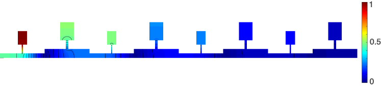
To confirm this subwavelength topological edge wave we have performed the numerical computation of eigenfrequencies and eigenmodes of a cavity closed by hard walls. It solves the 2D Helmholtz equation with Neumann boundary conditions at the walls, using Finite Element Method. We follow the approach described previously, but take an even number of segments (), which allows us to isolate one unique edge mode Coutant et al. (2021a) at the extremity with the smallest width (here ). Each segment is decorated by an Helmholtz resonator with neck width , neck length and a cavity of width and height . These geometrical parameters are finely tuned to get an equal Bloch phase following equation (21) in the range of frequencies , for both segments of cross section and . The values of these tuned paramters are found to be , , , , and , , , , ; they correspond to resonance frequency and a coupling parameter . The corresponding edge mode is confirmed to appear (it is the fifth mode of the cavity) and is displayed in Fig. 5. It can be remarked that the amplitude is strongly concentrated in the first resonator at the left.
IV Remark: resonators in series by inverse design
Interestingly, now that we understood the structure of the subwavelength edge mode (shown in Fig. 4(c)), we can reverse engineer it to obtain alternative structures also hosting a subwavelength edge mode.
We now show how this can be done in an array of only waveguide segments of changing cross-section. First, we assume that we work at low frequencies, such that the pressure profile is piecewise linear (as in Fig. 4(c)). Let us start at the left wall, where the pressure derivative vanishes. Because of that boundary condition, the pressure profile in the first segment, of section is flat. We then put a segment of section , so that the pressure derivative at jumps from a near-zero value to a non-zero one. Since the profile in the first segment is not exactly flat, a small shift of frequency changes the near-zero derivative at . The edge mode is such that the pressure slope in the second segment leads to a vanishing pressure at . Here, we put another segment , so that the pressure derivative decreases in amplitude. Now, the fourth segment has a section satisfying , so that the pressure derivative becomes almost zero in that segment. Doing so, at the fifth section change, pressure is maximum and hence no jump of derivative occur, and we can put a segment of section again. However, we need to flip the sign of the (near-zero) derivative, and hence, we must use . Doing so, the profile is back to its initial structure with an overall decrease of amplitude. By repeating the construction, we see that the pressure amplitude decreases for each set of four segment, and hence we obtain an edge mode, which by construction has a low (subwavelength) frequency.
Because a picture is worth a thousand words, we show the edge mode in such a configuration in Fig. 6. Notice that each large change of cross-section can be seen as a Helmholtz resonator. Hence, the described configuration amonts to Helmholtz resonators in placed in series, and inducing an edge mode near their resonance frequency.
Remarkably, while we have built a construction made of a set of four segments repeated along the waveguide, the same construction can be generalized to any values of cross-sections (e.g. in disordered configurations) as long as the inequalities exposed above are still valid. Explicitly, if we call the section of the segment, we need , , , and . For completeness, we now give the discrete set of equation relating pressure at each cross-section change (more details for the derivation can be found in Coutant et al. (2021a), section IV):
| (23a) | |||||
| (23b) | |||||
| (23c) | |||||
| (23d) | |||||

V Conclusion
In a previous work it was shown that a one-dimensional acoustic waveguide with alternating cross sections can be mapped exactly to the SSH lattice model Coutant et al. (2021a). Here, we extend this mapping by adding extra scatterers inside each segment of the waveguide. We show that the mapping is governed by a relation between the energy eigenvalue of the lattice model and the acoustic frequency, which now involves the Bloch phase accumulated along a segment (equivalently, the acoustic path), see equation 17. Using this extended relation, we consider a configuration where Helmholtz resonators are added on the wall of each segment. Near the resonance frequency, it is now possible to obtain large Bloch phases. As a consequence, the topological edge mode of the SSH model, that has zero energy, is mapped to an acoustic mode whose frequency can be tuned at will. In particular, we obtain topologically protected modes at an arbitrarily low frequency.
Moreover, our setup offers a much larger degree of control of the mode properties than previous proposals of a subwavelength topological mode Li et al. (2020); Zhao et al. (2021). Indeed, based on the exact mapping to the SSH model, the cross section changes and the Helmholtz resonators parameters govern distinct and well identified aspects of the system. For instance, the eigenfrequency of the edge mode is entirely controlled by the resonators characteristics, but insensitive to the cross section values, which in turn can be used to change the size of the corresponding gap.
References
- Huber (2016) S. D. Huber, Nature Physics 12, 621 (2016).
- Zhang et al. (2018) X. Zhang, M. Xiao, Y. Cheng, M.-H. Lu, and J. Christensen, Communications Physics 1, 1 (2018).
- Ozawa et al. (2019) T. Ozawa, H. M. Price, A. Amo, N. Goldman, M. Hafezi, L. Lu, M. C. Rechtsman, D. Schuster, J. Simon, O. Zilberberg, et al., Reviews of Modern Physics 91, 015006 (2019).
- Delplace and Venaille (2020) P. Delplace and A. Venaille, Comptes Rendus. Physique 21, 165 (2020).
- Xiao et al. (2014) M. Xiao, Z. Zhang, and C. T. Chan, Phys. Rev. X 4, 021017 (2014), eprint 1401.1309.
- Xiao et al. (2015) M. Xiao, G. Ma, Z. Yang, P. Sheng, Z. Zhang, and C. T. Chan, Nature Physics 11, 240 (2015).
- Xiao et al. (2017) Y.-X. Xiao, G. Ma, Z.-Q. Zhang, and C. T. Chan, Phys. Rev. Lett. 118, 166803 (2017).
- Meng et al. (2018) Y. Meng, X. Wu, R.-Y. Zhang, X. Li, P. Hu, L. Ge, Y. Huang, H. Xiang, D. Han, S. Wang, et al., New Journal of Physics 20, 073032 (2018), eprint 1804.10754.
- He et al. (2016) C. He, X. Ni, H. Ge, X.-C. Sun, Y.-B. Chen, M.-H. Lu, X.-P. Liu, and Y.-F. Chen, Nature physics 12, 1124 (2016), eprint 1512.03273.
- Yves et al. (2017) S. Yves, R. Fleury, F. Lemoult, M. Fink, and G. Lerosey, New Journal of Physics 19, 075003 (2017).
- Li et al. (2020) Z.-w. Li, X.-s. Fang, B. Liang, Y. Li, and J.-c. Cheng, Physical Review Applied 14, 054028 (2020).
- Zhao et al. (2021) D. Zhao, X. Chen, P. Li, and X.-F. Zhu, AIP Advances 11, 015241 (2021).
- Coutant et al. (2021a) A. Coutant, A. Sivadon, L. Zheng, V. Achilleos, O. Richoux, G. Theocharis, and V. Pagneux, Phys. Rev. B 103, 224309 (2021a), eprint 2103.03859.
- Su et al. (1979) W. Su, J. Schrieffer, and A. J. Heeger, Phys. Rev. Lett. 42, 1698 (1979).
- Asbóth et al. (2016) J. K. Asbóth, L. Oroszlány, and A. Pályi, Lecture notes in physics 919, 87 (2016), eprint 1509.02295.
- Zheng et al. (2019) L.-Y. Zheng, V. Achilleos, O. Richoux, G. Theocharis, and V. Pagneux, Physical Review Applied 12, 034014 (2019).
- Zheng et al. (2020) L.-Y. Zheng, V. Achilleos, Z.-G. Chen, O. Richoux, G. Theocharis, Y. Wu, J. Mei, S. Felix, V. Tournat, and V. Pagneux, New Journal of Physics 22, 013029 (2020).
- Coutant et al. (2020) A. Coutant, V. Achilleos, O. Richoux, G. Theocharis, and V. Pagneux, Phys. Rev. B 102, 214204 (2020), eprint 2007.13217.
- Coutant et al. (2021b) A. Coutant, V. Achilleos, O. Richoux, G. Theocharis, and V. Pagneux, Journal of Applied Physics 129, 125108 (2021b), eprint 2012.15168.
- Markos and Soukoulis (2008) P. Markos and C. M. Soukoulis, Wave propagation: from electrons to photonic crystals and left-handed materials (Princeton University Press, 2008).