Substructures in the Disk-Forming Region of the Class 0 Low-Mass Protostellar Source IRAS 162932422 Source A on a 10 au Scale
Abstract
We have observed the Class 0 protostellar source IRAS 162932422 A in the C17O and H2CS lines as well as the 1.3 mm dust continuum with the Atacama Large Millimeter/submillimeter Array at an angular resolution of 01 (14 au). The continuum emission of the binary component, Source A, reveals the substructure consisting of 5 intensity peaks within 100 au from the protostar. The C17O emission mainly traces the circummultiple structure on a 300 au scale centered at the intensity centroid of the continuum, while it is very weak within the radius of 50 au from the centroid. The H2CS emission, in contrast, traces the rotating disk structure around one of the continuum peaks (A1). Thus, it seems that the rotation centroid of the circummultiple structure is slightly different from that of the disk around A1. We derive the rotation temperature by using the multiple lines of H2CS. As approaching to the protostar A1, the rotation temperature steeply rises up to 300 K or higher at the radius of 50 au from the protostar. It is likely due to a local accretion shock and/or the preferential protostellar heating of the transition zone from the circummultiple structure to the disk around A1. This position corresponds to the place where the organic molecular lines are reported to be enhanced. Since the rise of the rotation temperature of H2CS most likely represents the rise of the gas and dust temperatures, it would be related to the chemical characteristics of this prototypical hot corino.
1 Introduction
Recently, rotationally-supported disks are found not only in Class I sources but also in some Class 0 sources (e.g. Yen et al., 2013, 2017; Murillo et al., 2013; Ohashi et al., 2014; Tobin et al., 2015, 2016a, 2016b; Seifried et al., 2016; Lee et al., 2017; Aso et al., 2017; Okoda et al., 2018). In spite of these extensive efforts, it is still controversial when and how a disk structure is formed around a newly born protostar. Moreover, the disk formation process has been revealed to be much more complicated for binary and multiple cases both in observations (Tokuda et al., 2014; Dutrey et al., 2014; Takakuwa et al., 2014, 2017; Tobin et al., 2016a, b; Boehler et al., 2017; Artur de la Villarmois et al., 2018; Alves et al., 2019) and numerical simulations (e.g. Bate & Bonnell, 1997; Kratter et al., 2008; Fateeva et al., 2011; Shi et al., 2012; Ragusa et al., 2017; Satsuka et al., 2017; Price et al., 2018; Matsumoto et al., 2019). For instance, circumbinary/circummultiple disk structures with a spiral structure as well as a circumstellar disk for each component are reported (e.g. Tobin et al., 2016b; Takakuwa et al., 2017; Artur de la Villarmois et al., 2018; Matsumoto et al., 2019; Alves et al., 2019). In addition, it is not clear how molecules are processed during the disk formation process and what kinds of molecules are finally inherited to protoplanetary disks and potentially to planets. Understanding these processes is crucial, as they will provide important constraints on the initial physical and chemical conditions for the planetary-system formation study. In this context, physical and chemical structures and their mutual relation for disk-forming regions of low-mass protostellar sources have been investigated with ALMA (Atacama Large Millimeter/submillimeter Array) (e.g. Sakai et al., 2014a, b; Oya et al., 2016, 2017, 2018, 2019; Imai et al., 2016, 2019; Jacobsen et al., 2019). These studies reveal that infalling envelopes and rotationally-supported disks are not smoothly connected to each other both in physical structure and chemical composition unlike previous expectations.
IRAS 16293–2422 is a well-studied low-mass protostellar source located in Ophiuchus ( 140 pc; Ortiz-León et al., 2017). It is a Class 0 binary system, consisting of Source A and Source B, which are separated by 5″. Both the components are famous for their richness in complex organic molecules (COMs) and are known as hot corinos (e.g. van Dishoeck et al., 1995; Cazaux et al., 2003; Schöier et al., 2002; Bottinelli et al., 2004; Kuan et al., 2004; Ceccarelli, 2004; Chandler et al., 2005; Caux et al., 2011; Jørgensen et al., 2012). Recently, the chemical characteristics of Source B has extensively been investigated by the PILS (Protostellar Interferometric Line Survey) program with ALMA (e.g. Coutens et al., 2016; Jørgensen et al., 2016; Lykke et al., 2017; Manigand et al., 2020b). As well, the characteristics of Source A has recently been reported by Manigand et al. (2020a) in the same program. Meanwhile, Source A was investigated in terms of the kinematic structures; the rotating signature of the gas surrounding the protostar was detected thanks to its nearly edge-on configuration (e.g. Pineda et al., 2012; Favre et al., 2014). Oya et al. (2016) reported that the kinematic structure of the gas in the vicinity of the protostar in Source A can be disentangled into the two major components; the infalling-rotating envelope and the rotating disk. They evaluated the protostellar mass ( ) and the specific angular momentum of the infalling-rotating envelope ( km s-1 pc) of this source under the assumption of the inclination angle of 60° (0° for a face-on configuration). The transition from the infalling-rotating envelope to the rotating (Keplerian like) disk was found to be occurring at the radius of au from the center of gravity, which corresponds to the radius of the centrifugal barrier of the infalling-rotating envelope. The chemical composition of the gas was found to change drastically in this transition zone.
The chemical evolution in protostellar sources is tightly related to the physical condition, and especially, the gas temperature distribution is of particular importance for its understanding. The temperature distribution in IRAS 16293–2422 has recently been modeled by Jacobsen et al. (2018); their 3D model of the dust and gas surrounding IRAS 16293–2422 Source A and Source B explains the observed distributions of the CO isotopologue lines and the dust emission. The gas dynamics connecting Source A and Source B has also been reported by van der Wiel et al. (2019). As for Source A, Oya et al. (2016) and van’t Hoff et al. (2020) derived the temperature structure on a au scale by analyzing the intensity ratios of -structure lines of H2CS observed at a 05 resolution (70 au). The result is discussed in relation to the drastic chemical change found on a 50 au scale mentioned above (Oya et al., 2016). Detailing a possible substructure in the transition zone is important for understanding the initial condition of the physical/chemical evolution in the disk formation process. However, the previous observations (Oya et al., 2016; van’t Hoff et al., 2020) do not have a sufficient spatial resolution (05; 70 au) for this purpose. In this study, we make use of the ALMA data observed at a high spatial resolution (01; 14 au) and have a close look at the disk/envelope structure of IRAS 16293–2422 Source A with particular emphasis on its substructure and gas-temperature distribution. We note that Maureira et al. (2020) have very recently reported a high resolution observation at 3 mm with ALMA, which can be compared with this study.
We summarize the observation in Section 2 and its overall results in Section 3. We present the kinematic structure of the gas around Source A in Section 4, and the gas temperature distribution in Section 5. Then, we discuss possible interpretations for the disk/envelope system of Source A in Section 6. The major conclusions are summarized in Section 7.
2 Observations
Our observations toward IRAS 16293–2422 were carried out on 21st August 2017 with ALMA during its Cycle 4 operation. Forty-four antennas were used in the observations. We employed the Band 6 receiver to observe the spectral lines of C17O and H2CS (Table 1). The field center of the observations was set to IRAS 16293–2422 Source A, which is located at . The baseline lengths of the antennas ranged from 21.0 to 3696.9 m. The size of the field of view was 2515, and the typical size of the synthesized beam was 01 for each image (see Table 1). The largest recoverable angular scale was 227. The total on-source time was 70.6 minutes. Four spectral windows were observed. Their spectral resolution and the band width are summarized in Table 2. The bandpass calibration was performed with J1517-2422, while the phase calibration was performed with J1625-2527 every 2 minutes. J1517-2422 and J1733-1304 were observed to derive the absolute flux density scale. The absolute accuracy of the flux calibration is expected to be better than 15 % (ALMA Partnership, 2016).
The continuum and line images were obtained with the CLEAN algorithm. We employed the Briggs weighting with a robustness parameter of 0.5, unless otherwise noted. The 1.3 mm continuum image was prepared by averaging line-free channels, whose total frequency range was 0.3 GHz. The line maps were obtained after subtracting the continuum component directly from the visibility data. The line maps were resampled to make the channel width to be 0.2 km s-1. A primary beam correction was applied to the continuum and the line maps. The root-mean-square (rms) noise level is 0.3 mJy beam-1 for the continuum map, while it is 2.5 and 2.0 mJy beam-1 for the C17O and H2CS line images, respectively. The velocity channel maps of the molecular lines were obtained by smoothing the velocity width of 1 km s-1 so that the rms noise level is 1.1 and 0.9 mJy beam-1 for the C17O and H2CS line images, resepctively. We tried self-calibration in various ways. However, the images are not improved or even deteriorated. Since we discuss the proper motion of the continuum peaks, we employ the images without self-calibration in this paper.
3 Results
3.1 1.3 mm Continuum
Figure 1(a) shows the 1.3 mm dust continuum image of IRAS 16293–2422. The continuum emission of Source A extends along the northeast-southwest direction (Figure 1b). Its elongated shape suggests the nearly edge-on configuration of Source A (e.g. Huang et al., 2005). Moreover, it shows substructures. We identify five intensity peaks, as shown in Figure 1(b). Their positions and peak intensities are listed in Table 3. These values are obtained by using the 2D Fit Tool of casa viewer. Although IRAS 16293–2422 is known to have a bridge structure connecting between Source A and Source B (e.g. Jørgensen et al., 2016; van der Wiel et al., 2019), such a structure is missing in our observation probably due to the resolving-out effect.
In order to have a careful look at the clumpy structure of the 1.3 mm continuum emission, we prepare the continuum image cleaned with a uniform weighting for a better spatial resolution. Figure 1(c) depicts the continuum image obtained with the uniform weighting. The angular resolution of the image with a uniform weighting is (0106 0064) ( 14 au 9 au), which is slightly better than that with the Briggs weighting (0128 0080; 18 au 11 au). With the uniform weighting, the intensity peaks A1, A2, A3, and A4 are clearly resolved as well as in Figure 1(b). In addition, the peak A1a spatially separated from the nearby peak A1 is tentatively detected. Figure 1(d) shows the spatial profile of the continuum emission along the line passing the peak A1 and A1a. The separation between A1 and A1a is clearer in the image with the uniform weighting. Although the uniform weighting (Figure 1c) provides a slightly better resolution than the Briggs weighting (Figure 1b), the resolved-out effect increases due to less contribution of short-baseline data. Because we are interested in the structure surrounding Source A, we hereafter employ the continuum image with the Briggs weighting (Figures 1b), which better traces the extended disk/envelope system.
The two continuum peaks in Source A (A1, A2) were reported in the 2 cm (15 GHz) continuum image observed with VLA (Very Large Array) by Wootten (1989). More clumpy features of Source A has recently been reported in the 2 cm (15 GHz) and 0.9 cm (33 GHz) continuum images observed with VLA by Hernández-Gómez et al. (2019). Figures 2(a) and (b) show their cm continuum images overlaid on our mm continuum image. They reported the proper motion of these continuum peaks based on the VLA data performed from 1986 to 2015 (Chandler et al., 2005; Pech et al., 2010), except for the peak A2. Figure 2(c) shows the extrapolation of the proper motion from the VLA observation in February 2014 (2014.15) to our ALMA observation in August 2017 (2017.64). Although calibration errors in the observations may affect the peak positions, the continuum peaks A1 and A2 observed with VLA in 2014 seem to correspond to those observed with ALMA in 2017. Very recently, the proper motion of A1 and A2 is also discussed by Maureira et al. (2020).
It has been thought that Source A is a candidate of a multiple system based on its multiple outflow structures (e.g. Stark et al., 2004; Yeh et al., 2008; van der Wiel et al., 2019; Maureira et al., 2020). In fact, the continuum peaks A1 and A2 have been interpreted as protostars constituting a close binary system (Loinard et al., 2007; Pech et al., 2010; Hernández-Gómez et al., 2019), although A1 was also suggested to be a shock feature (Wootten, 1989; Chandler et al., 2005). On the other hand, the continuum peaks A2 and A2 observed with VLA are interpreted as bipolar ejecta moving away from the protostar A2 (e.g. Hernández-Gómez et al., 2019). These two components (A2 and A2) seem missing in our ALMA observation considering their proper motion, although the continuum peak A3 detected with ALMA coincides with the A2 position observed in 2014 (Hernández-Gómez et al., 2019). The continuum peaks A3 and A4 (and A1a) detected with ALMA do not seem to have corresponding components in the VLA images. These peaks are not clearly seen in the 3 mm continuum image by Maureira et al. (2020), although a weak extended emission is seen around them. On the other hand, the peak A3 seems to correspond to Ab in the 1.3 mm continuum image reported by Sadavoy et al. (2018) (see also Chen et al., 2013; Chandler et al., 2005). The nature of the continuum peaks will be discussed later (Sections 4.1 and 4.4).
3.2 Molecular Lines
In this observation, we detected various molecular lines as in the other observations toward this source (e.g. Jørgensen et al., 2016). Among them, we focus on the C17O and H2CS lines in this study to characterize the gas distribution and the temperature distribution. Their line parameters are summarized in Table 1. Figure 3 shows their integrated intensity maps.
3.2.1 C17O
The distribution of the C17O ( = 2–1) line is extended along the distribution of the continuum emission over 300 au in diameter (Figure 3a). Although the signal-to-noise ratio of the integrated intensity map is not so high partly due to the resolved-out effect, the C17O emission seems to trace the the outer region of the continuum distribution. Figure 3(b) shows the velocity map (moment 1 map) of the C17O line. The velocity gradient is clearly seen along the northeast-southwest direction; the emission is blue-shifted in the northeastern side, while it is red-shifted in the southwestern side. The velocity gradient is almost parallel to the elongation of the distribution of the continuum emission. It seems to trace the rotating motion, which is consistent with the previous works (e.g. Pineda et al., 2012; Favre et al., 2014; Oya et al., 2016).
Figure 4 shows the velocity channel maps of the C17O line. The C17O emission is detected with the confidence level of 10 (11 mJy beam-1) or higher for the velocity range from to 9 km s-1, or the velocity shift between km s-1 from the systemic velocity of 3.9 km s-1. Additional emission features are seen in panels for the velocity range from to km s-1 and from 13 to 15 km s-1. These are contaminations of the (CH3)2CO (– EE and – EE at 224.700 GHz) transitions, the CH2DOH (–, e1 at 224.701 GHz; –, e1 at 224.725 GHz) lines, and/or an unidentified line. An absorption feature of the C17O line is seen around the systemic velocity, which is likely due to the self-absorption by the cold foreground gas. As seen in the velocity map (Figure 3b), the rotation signature can be confirmed in the velocity channel maps.
3.2.2 H2CS
Figures 3(c), (d), and (f) show the distributions of the H2CS lines. We detected the six -structure lines of H2CS with the upper energy levels from 46 to 375 K as listed in Table 1, although the highest transitions (–, –) are contaminated with the – line (see Section 4.4). All the H2CS line emissions show their intensity peak near the A1 continuum peak in contrast to the C17O ( = 2–1) line. Figure 3(e) shows the velocity map of the H2CS (–) line. The velocity gradient due to the rotation is clearly seen as the C17O line case.
Figure 5 shows the velocity channel maps of the H2CS (–) line. Here, we employ this line because the low-excitation line (–) is contaminated with the H2CS (–, –) line (see Section 4.4). In contrast to the C17O ( = 2–1) line case, a self-absorption feature is not seen near the systemic velocity. The H2CS (–) emission is detected with the confidence level of 10 (9 mJy beam-1) or higher for the velocity range from to km s-1, or the velocity shift from to km s-1. The velocity range is wider than that of the C17O ( = 2–1) line. The high velocity blue-shifted emission is present on the northeastern side of A1, while the high velocity red-shifted emission is on the southwestern side. They likely traces the rotating motion around the protostar A1. On the other hand, a clump is seen between the continuum peaks A2 and A4 in panels for the velocity from 8 to 12 km s-1. This component can also be seen in the integrated intensity maps of the H2CS lines as a shape of ‘tongue’ from A1 (Figures 3c, d, f). It is highly red-shifted near the continuum peak A4 in the velocity map (Figure 3e). We discuss this component in Sections 4.4.4 and 5.
4 Analysis and Discussion
4.1 Substructures of the 1.3 mm Continuum Emission
As described in Section 3.1, IRAS 16293–2422 Source A is a multiple system including at least two protostars A1 and A2 (Figure 1). Observational researches of binary and multiple systems have recently been reported (Tokuda et al., 2014; Takakuwa et al., 2014, 2017; Tobin et al., 2016a, b; Boehler et al., 2017; Artur de la Villarmois et al., 2018; Alves et al., 2019). The radio continuum emission observed toward binary/multiple systems shows various substructures; for instance, L1551 NE has a circumstellar disk for each constituent of the binary and arm structures surrounding the binary system (Takakuwa et al., 2017), while [BHB2007] 11 has circumstellar disks connected to a circumbinary disk by spiral streamers (Alves et al., 2019). Numerical simulation studies for circumstellar disks indeed reproduce such substructures (e.g. Bate & Bonnell, 1997; Fateeva et al., 2011; Satsuka et al., 2017; Price et al., 2018; Matsumoto et al., 2019). Both the observational and theoretical researches suggest a spatial gap of the gas distribution between the circumbinary disk and the circumstellar disks. These structures are thought to be caused by gravitational instability due to rotation and/or turbulence of a parent core (e.g. Bate et al., 2003; Matsumoto & Hanawa, 2003; Lim et al., 2016).
In Figure 2, the 1.3 mm continuum emission traces substructures similar to those observed previously with VLA (Hernández-Gómez et al., 2019). The weak extended component on a 300 au scale shown in Figure 1(b) seems to be a circumbinary/circummultiple envelope or disk, while each protostar inside it may be associated with a circumstellar disk revealed by a local emission peak. Our current observation does not show an apparent spiral or arm structure potentially existing in the circummultiple structure, although the continuum peak A1a extended from A1 may be a hint of such inner structures. In the following sections, we investigate the physical and kinematic structures of the circummultiple structure and possible circumstellar disks.
4.2 Morphological Structure of the Disk/Envelope System
The overall distribution of the 1.3 mm dust continuum emission in Source A looks like an ellipse (Figure 1), whose major axis extends along the northeast-southwest direction. It is necessary to define the center position and the major and minor axes of the distribution in order to investigate the kinematic structure of the gas showing the rotation signature. However, this process is not straightforward, because the dust continuum distribution has substructures. Thus, we derive them in the following way. First, we determine the centroid of the continuum intensity distribution using the data points with 3 (0.9 mJy beam-1) detection or higher to be the following: . The data points used for this calculation are within the magenta contour in Figure 6(a). Then, we fit the positions of the data points used above to an ellipse by using the least-squares method weighted by the intensity at each position. The centroid of the ellipse is found to coincide with the intensity centroid obtained above within the pixel size of the map (0025). The major and minor axes are derived in the above fit to be 125 (170 au) and 050 (70 au), respectively, while the position angle (P.A.) of the major axis of the elliptic distribution to be . This ellipse is shown in Figure 6(a). Thus, we assume that the mid-plane of the disk/envelope system extends along the P.A. of 50° (hereafter ‘the envelope mid-plane direction’). If a flat disk structure without thickness is assumed, its inclination angle is roughly estimated to be 66° (0° for a face-on configuration) from the ratio of the sizes of the major and minor axes. This value can be regarded as a lower limit to the inclination angle, if a finite thickness and a round shape for the disk structure are considered. Thus, the disk/envelope system of IRAS 16293–2422 Source A is confirmed to be nearly or almost edge-on as reported previously (e.g. Pineda et al., 2012; Favre et al., 2014; Oya et al., 2016). The envelope mid-plane direction and the intensity centroid determined above are shown in Figure 6(a) by a white arrow and a black cross, respectively. The intensity centroid can be regarded as a rough estimate of the center of gravity for the elliptic structure, assuming that the intensity of the dust emission is proportional to the dust mass at each position.
Figure 7(a) shows the spatial profiles of the continuum intensity and the integrated intensities of the molecular lines along the envelope mid-plane direction. The continuum emission shows a peak at the angular offset of 0″ (the intensity centroid of the continuum emission), which corresponds to the skirt of the A1 peak. It also has an additional peak at the angular offset of (40 au), which corresponds to that of the A3 peak. Similarly, the H2CS (–; –; –, –) emissions have a peak at the angular offset of 0″ with a shoulder or another peak at the offset of 02. Thus, these emissions are centrally concentrated. On the other hand, the C17O ( = 2–1) emission is more extended than the continuum and the H2CS emissions and shows a double-peaked feature with a depression of its intensity in the area inward of 50 au from the centroid (the interior of the two dotted lines in Figure 7a), where the continuum and the H2CS emissions are the brightest.
4.3 Kinematic Structure of the C17O Line
We first focus on the double-peaked distribution of the C17O ( = 2–1) emission and analyze its kinematic structure. Figure 8 shows the position-velocity (PV) diagrams of the C17O line prepared along the 6 directions shown by arrows in the attached velocity map, which are centered at the intensity centroid of the continuum emission. In the PV diagram along the envelope mid-plane direction (Figure 8a), we see the spin-up feature toward the intensity centroid of the continuum emission; the velocity gets more red-shifted from the systemic velocity (3.9 km s-1) as approaching to the protostar position from the southwestern side, while it gets more blue-shifted as approaching from the northeastern side. Interestingly, this feature almost vanishes inward of 04 (50 au) from the continuum peak position. This corresponds to the position where the integrated intensity of the C17O line decreases (Section 4.2; Figure 7a).
We also inspected the velocity structure of the C17O line around the continuum peak A1 as in the case of the H2CS lines, which will be described in Section 4.4. We found that the C17O emission does not show a symmetric feature around A1 in contrast to Figure 8. Therefore, we concluded that the center for the kinematic structure of the C17O emission should be at the center of gravity of the elliptic structure traced by the dust continuum emission, rather than at A1.
In this section, we compare the observed kinematic structure with two simple models which have often been used in previous studies. We here use three-dimensional physical models of a flat disk/envelope with the Keplerian motion or the infalling-rotating motion. The details for these models are reported by Oya et al. (2014) (Oya, 2017; Oya and Yamamoto, in prep.). In these models, the line emission is assumed to be optically thin, and the radiation transfer is not considered. Free parameters are the protostellar mass and the inclination angle for the Keplerian model, while the infalling-rotating envelope model has the radius of the centrifugal barrier as a free parameter in addition to them. We conduct the chi-squared () test for the two models to obtain the reasonable parameters. The details for the reduced test are described in Appendix A. The best fit and the reasonable ranges for the parameters are summarized in Table 4.
4.3.1 Keplerian Model for the C17O Line
First, we examine the Keplerian model for the PV diagrams of C17O. We optimize the protostellar mass and the inclination angle as free parameters to explain the observed PV diagrams. Although the reduced values suffer from the imperfection of the model and the complexity of the sources, we obtain the following best fit parameters of the Keplerian model: the central mass is 2.0 and the inclination angle is 70°, as shown in Table 4. Here, the inner and outer radii of the model are fixed to be 50 au and 300 au according to the observed molecular distribution. Other details of the fittings are described in Appendix B.
Figure 8 shows the PV diagrams of the Keplerian model with the best fit parameters. As depicted in Figure 8(a), the PV diagram along the envelope mid-plane direction is reasonably reproduced. However, the PV diagrams along the other directions are not well explained, although their overall trend is roughly reproduced (Figures 8b–f). The resolved-out effect and/or the self-absorption effect would affect the velocity components near the systemic velocity (3.9 km s-1); the observation does not show emission while the model does. On the other hand, there are some parts in the PV diagrams where the line emission is detected but is not reproduced by the model. Such discrepancy originates from the imperfection of the model. For instance, the model cannot well explain the PV diagram along the direction perpendicular to the envelope mid-plane direction (Figure 8d). The blue-shifted component in Figure 8(d) has a higher velocity-shift in the observation than the model.
4.3.2 Infalling-Rotating Envelope Model for the C17O Line
Next, we examine the infalling-rotating envelope model (Oya et al., 2014). In this model, the velocity field is approximated by the ballistic motion. The energy and specific angular momentum of the gas is assumed to be conserved, and thus the gas cannot fall inward of the periastron, which is called as the ‘centrifugal barrier’. The following best fit parameters for the infalling-rotating envelope model are obtained: the protostellar mass is 1.0 and the inclination angle is 80°. The radius of the centrifugal barrier and the outer radius of the model are fixed to be 50 au and 300 au according to the observed molecular distribution. The results for the fittings are described in Appendix B.
Figure 9 shows the PV diagrams of the infalling-rotating envelope model with the best fit parameters. As in the case of the Keplerian disk model described above, the infalling-rotating envelope model does not explain the observed kinematic structure very well, either; for instance, the velocity-shift in the model is larger than the observed kinematic structure in Figures 9(c), (d), and (e). The PV diagrams along the envelope mid-plane direction is reasonably reproduced. However, the red-shifted component of the C17O ( = 2–1) line seems to severely suffer from the absorption effect by the infalling gas, so that a velocity gradient due to the infall motion expected along the direction perpendicular to the envelope mid-plane direction in the model is not evident in Figure 9(d).
4.3.3 Circummultiple Structure
Neither of the two simple models fully explains the detailed kinematic structure because of the complexity of the source. This source has the small substructures, which are now resolved in our observation. Hence, the kinetic structure would be too complicated to be modeled by these simple models. Although the infalling-rotating envelope model gives a smaller values than the Keplerian model (Tables A1 and A2), it would be too hasty to conclude that the C17O emission comes from an infalling-rotating envelope. Nevertheless, we can roughly constrain the central mass of Source A from the kinematic structure observed at the 01 resolution. Finer tuning of the model by, for instance, combining the two simple models is practically difficult, because such an analysis includes too many free parameters for our current observational data of this source, and it is out of scope of this work.
Then, we compare the protostellar masses derived above with those in the literatures. The protostellar mass of Source A is reported to be from 0.5 to 1.0 (e.g. Looney et al., 2000; Bottinelli et al., 2004; Huang et al., 2005; Caux et al., 2011; Pineda et al., 2012; Favre et al., 2014; Oya et al., 2016), while Takakuwa et al. (2007) and Maureira et al. (2020) reported a larger central mass from 0.5 to 2.0 . The central mass employed for the infalling-rotating envelope model above (1.0 ) is consistent with most of the previous reports. Meanwhile, the mass employed for the Keplerian model (2.0 ) agrees with the highest end of the previous reports.
As mentioned in Section 1, Oya et al. (2016) reported the infalling-rotating envelope structure with a radius of 300 au around Source A in the OCS emission at an angular resolution of . They suggested that the gas outside the radius of 50 au from the center of gravity is an infalling-rotating envelope while that inside the radius of 50 au is the Keplerian disk. If the C17O gas has the Keplerian motion rather than the infalling-rotating motion, the C17O gas would have a different kinematic structure from the OCS gas at the radius from 50 au to 300 au from the continuum intensity centroid, although the angular resolution of the OCS observation is coarser than that of the C17O observation. Thus, the OCS distribution could be somewhat different from the C17O distribution. For instance, if the envelope gas falls onto a thin rotating disk diagonally from above and below the mid-plane (e.g. Figures 4.5 and 4.11 in Hartmann, 2009), the OCS ( = 19–18) line with the high upper-state energy (111 K) will preferentially trace a warm surface of the infalling envelope gas. In contrast, the C17O ( = 2–1) line with the upper-state energy of 16 K tends to trace a cold dense mid-plane of the rotating disk, whose motion is close to be Keplerian.
The C17O emission seems to trace the circummultiple structure in Source A and is deficient in the vicinity of the center of gravity. A circumbinary disk is previously observed for L1448-IRS3B by Tobin et al. (2016b) in the 13CO ( = 2–1) emission with ALMA. Meanwhile, a hole of the 13CO distribution tracing the rotating gas is previously reported for TMC-1A by Harsono et al. (2018). They interpreted the hole structure as absorption of the 13CO emission by the optically thick dust. On the other hand, theoretical simulations show a gap of the gas distribution between a circumbinary disk and circumstellar disks (e.g. Bate & Bonnell, 1997; Fateeva et al., 2011; Satsuka et al., 2017; Price et al., 2018; Matsumoto et al., 2019). At the first glance, such a gap/hole structure would not be the case of the C17O emission in IRAS 16293–2422 Source A; in the C17O deficient area, the dust is not expected to be so optically thick as to significantly suppress the molecular emission enough, because the H2CS emission is observed there (Figure 3). However, an optically thick dust may cause the depression of the C17O emission if the molecular distribution is different between CO and H2CS (see next section for details).
4.3.4 C17O Deficiency within 50 au
The weak C17O ( = 2–1) emission near the centroid of the continuum emission (Figures 3a and 7a) is difficult to be interpreted by the freezing out of CO onto dust grains. In this area, the gas temperature is expected to be much higher than the desorption temperature of CO (20 K) according to the analysis of the H2CS line (see Section 5). If the dust temperature is also as high as the gas temperature, the weak emission of the C17O ( = 2–1) line cannot simply be attributed to the adsorption of CO onto dust grains.
The adsorption of CO might be the case, if the disk mid-plane temperature within 50 au were lower than the adsorption temperature of CO. On the other hand, the H2CS emission would mainly come from the warm region including the disk surface, and the effect of the depletion in the disk mid-plane could be less important. This picture qualitatively explains the behavior of the spatial profiles shown in Figure 7(a).
If such different distributions between CO and H2CS are the case, the optical depth effect of the continuum emission affects the C17O emission more seriously than the H2CS emissions. The C17O emission from the cold and dense mid-plane would be depressed by an optically thick dust, while the H2CS emissions from the warm surface region would be less affected. Such an effect of the optically thick dust was invoked for the 13CO hole observed in TMC-1A by Harsono et al. (2018).
The excitation effect can cause the weak C17O emission in the hot region in the vicinity of the continuum peak A1. In Figure 7(b), the integrated intensity is 49 mJy beam-1 km s-1 (120 K km s-1) and less than 3 (21 mJy beam-1 km s-1; 51 K km s-1) at its peak and A1, respectively. If the column density is the same for these two positions, the difference between these integrated intensities is explained by a factor of three difference of the excitation temperature (i.e., 100 K and 300 K for these two positions). Here the local thermodynamical equilibrium (LTE) condition and the optically thin condition are assumed. In this case, the excitation temperature would change sharply as the distance from the protostar, since the intensity of the C17O emission sharply changes.
Alternatively, non-volatile organic molecules formed in the gas-phase of the disk component are adsorbed onto dust grains, which may result in the exhaustion of carbon from the gas-phase (Aikawa et al., 1996). This might eventually cause deficiency of CO. In fact, IRAS 16293–2422 Source A is known to be rich in COMs. Moreover, Oya et al. (2016) reported that the COM emission is enhanced within the radius of 50 au, where the CO emission is weak in this observation. The deficiency in CO may be related to such peculiar chemical characteristics.
4.4 Kinematic Structure of the H2CS Lines
4.4.1 Rotating Disk around A1
In contrast to the C17O line, the H2CS lines are concentrated within the radius of 50 au (Figures 3c, d, f). In order to investigate this feature, we prepare the integrated intensity maps of the H2CS (–) line for the blue- and red-shifted velocity ranges (Figure 6b). Note that this line is free from significant contamination lines by other lines according to the spectral line database (JPL and CDMS; Pickett et al., 1998; Müller et al., 2005; Endres et al., 2016), which is also confirmed in the actual observations by van’t Hoff et al. (2020) and this work. Figure 6(b) shows the high velocity-shift components with the velocity shift from to km s-1. The rotation motion can be recognized around the continuum peak A1 rather than the intensity centroid of the dust continuum, although an additional red-shifted component is seen near the continuum peak A4. The blue-shifted and red-shifted components overlap just at the continuum peak A1. This result indicates the rotating structure associated with A1. Since the disk/envelope system of Source A shows substructures in its continuum emission, the center of gravity could be different between the envelope and this rotating structure. By focusing on the vicinity of A1, the P.A. of the velocity gradient due to the rotation is evaluated to be 50°. Thus, we assume that the mid-plane of the rotating structure around A1 extends along this P.A., which is parallel to the envelope mid-plane direction derived from the dust continuum distribution (Section 4.2). This direction (hereafter ‘the disk mid-plane direction’) is shown by a red arrow in Figure 6(b). Figure 7(b) shows the spatial profiles of the continuum emission and the integrated intensities of the molecular lines along the disk mid-plane direction. The continuum emission and the H2CS emission are concentrated to the continuum peak A1, while the C17O emission shows a double-peaked feature, as the spatial profiles along the envelope mid-plane direction (Figure 7a).
4.4.2 Keplerian Model for the H2CS Line
First, we perform the test for the Keplerian model and the H2CS (–, –) line, as the C17O case in Section 4.3.1 (see also Appendix A). We obtain the following best fit parameters: the central mass is 0.4 and the inclination angle is 60°, where the systemic velocity is 2.5 km s-1. The inner and outer radii of the model are fixed to be 0 au and 30 au according to the observed molecular distribution, respectively. We regarded the emission extending over 30 au as a part of the circummultiple structure traced by the C17O emission (Section 4.3), and we did not take them into account in the following analysis. The best fit and the reasonable ranges for the parameters are summarized in Table 4. Other details for the fittings are described in Appendix C.
Figure 10 shows the PV diagrams of the H2CS (–; –; –, –) lines along the directions with P.A.s of 50° and 80° centered at the protostar A1. The Keplerian model results with the best fit parameters obtained above is overlaid on the observation results. The PV diagrams of H2CS (–, –) along all the direction shown by the black arrows in the velocity map (moment 1 map) on the top left panel are shown in Appendix C (see Figure A5). We see the high velocity-shift components concentrated to the protostar A1. The PV diagrams in Figure 10 as well as those in Figure A5 can be reasonably explained by the Keplerian model described above, except for the three features particularly seen in Figures 10(b) and (d) (see Section 4.4.4).
4.4.3 Infalling-Rotating Envelope Model for the H2CS Line
Next, we performe the test for the infalling-rotating envelope model and the H2CS (–, –) line, as the C17O case in Section 4.3.2. We obtain the following best fit parameters: the central mas is 0.20 and the inclination angle is 70°, where the systemic velocity is 2.5 km s-1. The outer radius of the model is fixed to be 30 au according to the observed molecular distribution. The best fit and the reasonable ranges for the parameters are summarized in Table 4. Other details for the fittings are described in Appendix C. As the result, we find that the kinematic structure traced by H2CS is worse reproduced by the infalling-rotating envelope model than by the Keplerian model (Table 4; see Figure A8). Thus, the observed kinematic structure would prefer the Keplerian motion.
4.4.4 Comments on Additional Features
According to the model analysis in Sections 4.4.2 and 4.4.3, it is most likely that the continuum peak A1 is a protostellar source associated with a rotating disk structure. Some components detected in the H2CS emission are not attributed to this rotating disk structure. Figures 10(a) and (c) show low velocity-shift components extended from the angular offset of 02 to 1″. As we have described in Section 4.4.2, this component can be attributed to the circummultiple structure traced by the C17O emission (Figures 8, 9). Moreover, the observed PV diagrams show three features spilling over the model results, as we mentioned in Section 4.4.2.
An excess emission is seen at the velocity of about 12 km s-1 toward the A1 position (zero offset) in the PV diagram of the H2CS (–) line (‘Excess 1’ in Figure 10a, b). Since this feature is not seen in the H2CS (–, –) (Figure 10e, f) line, this emission is most likely interpreted as contamination by the unresolved doublet of H2CS (–, –). Although Oya et al. (2016) suggested an existence of the Keplerian disk component based on the observation of the H2CS (–) line, it would have suffered from this contamination (see also van’t Hoff et al., 2020). The H2CS (–) line shows a weak emission (‘Excess 2’) near Excess 1, too. Since it has a slight offset from the A1 position, it may be a contamination by another molecular line rather than a high velocity-shift component of the H2CS (–) line in the vicinity of the protostar. The peak intensity of this weak contamination is less than 30 % of that of the H2CS (–) line, and moreover, it is separated from the H2CS (–) line along the velocity axis. Therefore, the H2CS (–) line is verified to have no significant contamination by other molecular lines in its PV diagrams (Figure 10c, d), as noted in the previous sections. As well, this weak contamination does not affect the discussion for the rotation temperature of the H2CS in Section 5. Thus, we can certainly confirm the disk component with this line. It should be noted that the detection of the high-excitation line of H2CS (a composite of –, –; 375 K) suggests a high gas temperature of the disk component near the protostar A1.
Another excess emission in Figure 10(b) is the high-velocity component at an offset of from A1 (‘Excess 3’). This component can be seen in the H2CS (–, –, –) lines (Figure 10d, f), and cannot be ascribed to the contamination of the other lines. This component is neither the infalling-rotating envelope described in Section 4.3 nor the disk component around A1. It likely represents the component extended through the midway between A2 and A4 (see Section 3.2.2). This feature is interesting, because the velocity increases as an increasing distance from the protostar A1 (Figure 3e; see the 7–12 km s-1 panels of Figure 5). It might be a part of the outflowing motion. Alternatively, it looks like a part of a spiral structure (Figure 3f), as seen in circumbinary systems (Takakuwa et al., 2014, 2017; Matsumoto et al., 2019; Alves et al., 2019). Further characterization of this component is left for future study.
4.4.5 Comparison between the Circumstellar and Circummultiple Structures
We have also examined a possible disk structure associated with the other continuum peaks. For instance, Figure 11 shows the PV diagrams of the H2CS (–, –) line, where the position axes are centered at the protostar A2. If a molecular line traces a possible disk associated to A2, the PV diagrams have to be symmetric with respect to the A2 position and the systemic velocity of A2 (See Figures 8 and 9 for reference). However, such an expected feature is not evident in Figure 11. One may think that the kinematic structure in the panel (a) (P.A. of 50°) showing a velocity gradient can be interpreted as the Keplerian motion with a systemic velocity of 6 km s-1. In fact, Maureira et al. (2020) has recently suggested the existence of the rotating disk structure associated with the protostar A2. However, it is more adequately interpreted as a part of other components, i.e. the disk associated to A1 or the circummultiple structure of Source A in our observational result. At the current stage, we cannot conclude whether a rotating disk structure exists around the protostar A2. As well as the protostar A2, we have investigated the kinematic structure in the vicinity of the continuum peaks A3 and A4. Our current observation did not show a rotating disk structure around either of them.
Although the physical parameters in Table 4 are obtained with the simplified models, it is worth noting that the best fit masses, inclination angles, and systemic velocities are different between the circummultiple structure of Source A traced by the C17O ( = 2–1) emission and the circumstellar structure of the protostar A1 traced by the H2CS (–, –) emission. First, the central mass estimated for the circummultiple structure is from 1.5 to 2.5 with the Keplerian disk model and from 0.6 to 1.2 with the infalling-rotating envelope model. These values are larger than the central mass from 0.4 to 0.8 (the Keplerian model) and from 0.15 to 0.25 (the infalling-rotating envelope model) estimated for the circumstellar structure around A1. The circummultiple structure surrounds possible other components (A2, A3, A4, and A1a) as well as the protostar A1, and also their possible circumstellar structures. Thus, the central mass evaluated from the kinematic structure of the circummultiple structure should be higher than the mass evaluated for A1.
Maureira et al. (2020) have recently reported that the gas mass is , , and for the substructure around A1, that around A2, and the extended structure surrounding both of them, respectively, based on the 3 mm continuum emission. These values are significantly smaller than the difference of the central mass between the circummultiple and circumstellar structures found in this study. Thus, the mass of the rest sources, i.e. the protostar A2 and possible protostars A3 and A4, would contribute to the kinematic structure of the circummultiple structure.
Second, the inclination angle seems larger for the circummultiple structure than the circumstellar structure, although it has a large uncertainty. A1 is likely one component of a potential binary/multiple system of Source A. Thus, the differences of the inclination angle and the systemic velocity imply that the rotating disk structure around A1 could be tilted with respect to the circummultiple structure of Source A. As well, the difference of the systemic velocity between the two models, 3.9 km s-1 for the circummultiple structure and 2.5 km s-1 for the circumstellar structure, implies a potential motion of the protostar A1 in Source A.
5 Distribution of the Rotation Temperature of H2CS
In this section, we investigate the temperature distribution using the high spatial resolution data of H2CS. So far, the temperature structure on a au scale have been studied by Oya et al. (2016) and van’t Hoff et al. (2020) by using the -structure lines of H2CS observed at a 70 au resolution. The rotation temperature derived from these lines is a good measure of the gas kinetic temperature, because the radiation processes between the different levels () are very slow. Hence, they can be used for delineating the temperature structure around the protostar. Oya et al. (2016) derived the rotation temperature at the five positions with offsets of , , and 0″ from the continuum peak position, which correspond to the envelope, the transition zone (centrifugal barrier), and the disk, respectively, by using the intensity of the –, –, and –/– lines integrated over the velocity range corresponding to each component. Based on the result, they suggested the temperature rise at the transition zone by comparison of the temperatures at the five positions and discussed the result in relation to the enhancement of COMs near the transition zone. Later, van’t Hoff et al. (2020) observed more H2CS lines to derive the temperature structure of this source. They use the peak fluxes instead of the integrated intensity to derive the line ratio and delineate the temperature distribution in Source A. The temperature profile along the direction of the disk/envelope system does not reveal the local temperature rise suggested by Oya et al. (2016). Thus, they interpreted the temperature profile in terms of the radiation heating from the protostar. Although these works reveal the fundamental temperature distribution of this source, the spatial resolution is too coarse to examine the temperature structure around the transition zone in detail. Since substructures in the circummultiple system of Source A are now evident, we revisit the temperature structure of this source with the high resolution H2CS data. We here employ the H2CS (–) and (–, –) lines for the analysis, because the H2CS (–) line suffers from the contamination by the H2CS (–, –) lines. As we describe in Section 4.4.4, the weak contamination for the H2CS (–) line (Excess 2 in Figure 10c, d) does not matter as long as we discuss the line intensities with PV diagrams or velocity channel maps. The unresolved doublet of H2CS (–, –) is confirmed to have no significant contamination in the molecular line database and this observation (Figure 11), as the H2CS (–) line case mentioned in Section 4.4.4.
Figure 12(a) shows the distribution of the ratio of the integrated intensity of the H2CS (–, –) line relative to that of the H2CS (–) line, while Figure 12(b) shows the distribution of the rotation temperature of H2CS calculated from the integrated intensity ratio. Figures 13(a) and 14(a) show the spatial profiles of the integrated intensity ratio and the rotation temperature along the disk mid-plane direction (a red arrow in Figure 6b), respectively. Here, we assume the LTE condition and the optically thin conditions for the two lines. The LTE condition for H2CS is well fulfilled in this hot and dense region, as revealed with the non-LTE calculation by Oya et al. (2016). In order to verify the optically thin condition, we roughly calculate the optical depths of the H2CS (–) and (–, –) lines from the observed brightness temperature and the derived rotation temperature. Here, we ignore the contribution of the dust emission, because the treatment of this effect requires detailed radiation transfer and is out of the scope of this paper. The derived optical depths are mostly lower than 0.5, and its median is 0.28 and 0.10 for the H2CS (–) and (–, –) lines, respectively. The optical depth of the H2CS (–) line exceeds 1 for some parts. However, such high optical depth parts are in the low temperature regions (100 K). Since we discuss the temperature structure of hot components around the protostar, the optical depth effect does not affect seriously.
The rotation temperature of H2CS derived from the – and –/– lines is confirmed to be consistent with the gas kinetic temperature derived by using RADEX code (van der Tak et al., 2007) with the H2 density range of cm-3, which is relevant to disk/envelope systems (Oya et al., 2016). The rotation temperature of H2CS is evaluated to be as high as 300 K near A1. A high rotation temperature area is extended from A1 to southwestern part. The rotation temperature apparently decreases as the increasing distance from the protostar A1 position with a slight enhancement at the southwest part. These features are consistent with the result obtained at a lower spatial resolution by van’t Hoff et al. (2020). It is worth noting that the tongue-like feature from A1 (Section 3.2.2) shows high temperature (200 K; Figure 12b). As discussed in Section 4.4, this might be related to the outflowing motion.
We have also derived the rotation temperature from the intensity ratio of the – line to the – line for reference. The temperature is generally lower than that derived from the – and –/– lines. For instance, the former is 100 K and the latter is 200 K at the continuum peak A3. This is probably because the – line would sample colder regions and is partly contaminated by the H2CS (–, –) line (Section 4.4.4). Hence, we use the rotation temperature derived from the – and –/– lines in the following discussions.
Figure 15 shows the velocity channel maps of the rotation temperature of H2CS. Each map is derived based on the intensity ratio of the velocity channel maps of the H2CS (–) and (–, –) lines. As in Figure 12(b), the optically thin conditions for the two lines and the LTE condition are assumed. In Figure 12, the envelope and disk components are contaminated with each other along the line of sight, because the line emission is integrated for the velocity axis. On the other hand, they are expected to be disentangled to some extent in the velocity channel maps. In Figure 15, the rotation temperature of H2CS apparently becomes higher as approaching to the protostar A1 position. It is as high as 400 K near A1.
In the panels for the velocity of and km s-1 of Figure 15, the rotation temperature is as high as 400 K at some positions apart from the protostar A1. These positions roughly correspond to the positions within which the C17O emission decreases. Figures 16(a) and (b) show the maps of the highest intensity ratio of the two H2CS lines and the highest rotation temperature along the velocity channels, which are derived from the cube data. In other words, the maximum values along the line of sight are shown in these maps. These maps are obtained by using the immoments task of casa with the option “moments = [8]”. Figure 13(b) shows their spatial profiles along the disk mid-plane direction. The maximum intensity ratio along the line of sight steeply increases at the distance of 50 au from the protostar A1, and are almost constant within this radius. The highest rotation temperature along the line of sight shown in Figure 14(b) also steeply increases at the same position but shows a large scatter within it. It should be noted that very high temperatures obtained at some positions would be artificial. Since the intensity ratio at these positions are close to the high-temperature limit (1.47 for ) as shown in Figure 13(b), the derived temperature is sensitive to a small change in the ratio and suffers from a large error. Therefore, the intensity ratio itself better represents the temperature profile. Interestingly, the positions of the steep increase corresponds the transition zone from the circummultiple structure to the circumstellar structure, as mentioned above.
Thus, the local rise of the rotation temperature seems occurring near the transition zone from the circummultiple structure of Source A to the circumstellar structure of the protostar A1. A hint for such a temperature rise in the transition zone was previously suggested by Oya et al. (2016). However, this previous report would have been just fortuitous based on the results for a few positions, given the detailed analysis by van’t Hoff et al. (2020). Now, our high-resolution observation (01) indeed reveals a sharp change in the temperature. The local rise of the rotation temperature of H2CS most likely reflects a local rise of the gas temperature. Candidate mechanisms causing a local temperature rise are discussed in Section 6.
6 Transition from the Envelope to the Disk-Forming Region
When the radiation heating by the central protostar (A1) is considered as a heating source, the gas temperature is expected to gradually decrease as a power-law of the distance to the protostar. In the edge-on case, the maximum gas temperature along the line of sight is expected to be as well (Figure 17a). If the protostars other than A1 could contribute to the heating, the temperature profile would be more gentle than the case of the heating only by A1. This effect may contribute to flatten the temperature profile around A1 within the radius of 50 au. Nevertheless, it seems difficult to explain the local steep rise of the temperature on both the northeastern and southwestern sides of A1 by the protostellar heating alone. Thus, another heating mechanism is expected in IRAS 16293–2422 Source A.
The peak temperature profile projected onto the plane of the sky is expected to be flat, if the actual radial temperature profile is flat as well or it has a local rise in a ring-like structure. The observed temperature profile, which shows a steep rise around 50 au and then flattens, requires that the temperature is not significantly higher in the vicinity of the protostar than at the distance of 50 au from the protostar due to some mechanisms. The temperature is naturally expected to increase as approaching to the protostar by the radiation heating, and thus, a completely flat temperature profile within the radius of 50 au is unlikely. It seems more likely that the radial temperature profile has an increase at the radius of 50 au, drops just inside it, and gradually increases as approaching to the protostar.
If the local temperature rise just outside the circumstellar structure of A1 occurs due to an accretion shock by the infalling gas, it will appear in a ring-like structure surrounding the disk structure (Figure 17b). In fact, the model study by Fateeva et al. (2011) shows that bow-shocks can occur near the inner edge of a circumbinary disk. It may heat up the innermost edge of the circummultiple structure in IRAS 16293–2422 Source A. In the edge-on or nearly edge-on case, the maximum gas temperature along the ling-of-sight is expected to show a flat feature as a function of the distance from the protostar (A1). This corresponds to what can be seen in Figures 13(b) and 14(b).
Such a gas temperature distribution with a ring-like structure is also caused by a physical structure of the gas; the stagnated gas in the transition zone from the circummultiple structure to the curcumstellar structure can be piled up vertically to the mid-plane of the disk, and the gas is efficiently heated up by the radiation from the protostar without the shielding by the circumstellar disk structure (Figure 17b). In any case, the distribution of the rotation temperature in IRAS 16293–2422 Source A shown in Figure 16(b) seems consistent with the picture of the hot ring-like region.
The picture of the hot ring-like region would also be related to the local enhancement of the COM emission reported by Oya et al. (2016). The CH3OH emission and the HCOOCH3 emission likely come from the ring-like region with a radius of 50 au surrounding the protostar, based on their kinematic structures. According to Oya et al. (2016), the COM emission seems weaker in the circumstellar disk structure than at the transition zone. Although the spatial-resolution of their observation is insufficient, this distribution could be caused by the temperature distribution shown in Figure 17(b). COMs may be re-depleted onto dust grains because of the lower temperature of the disk mid-plane. If this picture is the case, the ‘hot corino’ would not have a simple spherical or disk-like structure in the vicinity of the protostar, but a ring-like structure surrounding the protostar. The gas and dust temperature will rise again in the closest vicinity of the protostar, and COMs can desorb from the dust grains there. Although one may think that the weak COM emission is due to the optically thick dust emission, it is not likely because the H2CS emission is strongly detected in the same area. As described in Section 4.3.4 for the C17O and H2CS case, this situation could be the case if H2CS and COM distribute in the gas phase of different parts of the disk/envelope system. To understanding the actual situation, it is required to confirm whether the distribution of the COM line emission is really weak within a certain radius. Observations of COM lines at a high spatial resolution will help us in this aspect, which are in progress. Observations at a lower frequency are favorable for this purpose in order to avoid the effect of dust opacity.
7 Summary
We have observed the Class 0 low-mass protostellar source IRAS 16293–2422 Source A in the C17O and H2CS lines as well as in the 1.3 mm dust continuum at a high angular-resolution of 01 (14 au). The major findings are as follows:
-
(1)
The 1.3 mm continuum emission traces the nearly edge-on disk/envelope system. Moreover, the substructures on a 05 (100 au) scale are resolved, and 5 continuum peaks are identified. The positions of two continuum peaks (A1 and A2) are consistent with those previously observed at cm wavelength, if their proper motions are considered. They also agree with the recent report on the 3 mm continuum emission. We also detect new continuum peaks (A3, A4, and A1a). Meanwhile, A2 and A2 observed at cm wavelength, which are thought to be the ejecta from A2, are missing. Thus, IRAS 16293–2422 Source A is likely a multiple system.
-
(2)
The C17O ( = 2–1) line emission traces the rotating gas on a 300 au scale centered at the intensity centroid of the dust continuum emission. On the other hand, C17O is found to be deficient within the radius of 50 au from the intensity centroid of the continuum emission. Enhancement of the temperature, depletion of CO onto dust grains in the mid-plane of the disk/envelope structure, and exhaustion of carbon to non-volatile organic molecules can be considered as the origin of this feature.
-
(3)
The multiple lines of H2CS mainly trace the disk component around the strongest continuum peak (A1). Even the high-excitation lines (–, –; 375 K) are detected.
-
(4)
The kinematic structures of the C17O and H2CS lines are examined by a Keplerian model and an infalling-rotating envelope model. The center of gravity, the inclination angle, and the systemic velocity of the circummultiple structure of Source A traced by C17O are possibly different from those of the circumstellar structure around the protostar A1 traced by H2CS.
-
(5)
The distribution of the rotation temperature of H2CS is derived. In an overall view, the rotation temperature increases as approaching to the protostar A1, as usually expected for the gas temperature profile determined by the radiation heating from the protostar. Interestingly, the rotation temperature shows a steep rise around the transition zone from the circummultiple structure to the circumstellar disk associated to the protostar A1. This local steep rise could be attributed to a possible accretion shock by the infalling gas and/or the thermal heating of the stagnated gas by the protostar. If the dust temperature rises there as well, it would be related to the rich COM emission, which is the chemical characteristics of IRAS 16293–2422 Source A. ‘Hot corino’ may have a ring-like structure, instead of a simple spherical or disk-like structure.
While theoretical studies have extensively progressed in the disk-formation study (e.g. Hennebelle, & Ciardi, 2009; Li et al., 2011; Machida et al., 2011; Tomida et al., 2015; Tsukamoto et al., 2017; Lam et al., 2019), observational studies tend to have been behind them due to the limited high-resolution observations. In these years, the radio observational studies have revealed the fundamental picture of the infalling-rotating envelope and the disk inside it, thanks to the unprecedented angular-resolution and the sensitivity of millimeter and submilimeter interferometers including ALMA. This work demonstrates that the transition zone from the circummultiple disk/envelope to the circumstellar disk is not smooth. Moreover, even substructures of the disk-forming region are now in the scope of the observations. Further study on these issues will provide us with deep insight into the formation process of the disk and the chemical evolution during it.
Appendix Appendix A Reduced Chi-Squared Test for the Position-Velocity Diagrams
In Sections 4.3 and 4.4, we conduct the chi-squared () test for the observed PV diagrams and the model results. We calculate the reduced value (/DOF), which is the sum of the square of the difference between the modeled and observed PV diagrams along the envelope mid-plane direction at each pixel normalized by the square of the rms in the observation (2.5 mJy beam-1 for C17O, 2.0 mJy beam-1 for H2CS).
A large reduced value mainly originates from complexity of the source and imperfection of the model. Hence, we should take relatively large ranges of the parameters which can reasonably reproduce the observed features. Based on this thought, the parameter ranges are determined from the range where the reduced value increases by 1. The best fit and the reasonable ranges for the parameters derived by the test are summarized in Table 4.
Appendix Appendix B Analysis of C17O
Since the C17O emission notably suffers from the self-absorption effect, we only use the blue-shifted component from km s-1 to km s-1 to calculate . Table A1 shows reduced for the central-mass versus inclination angle plane. Figure A1 shows examples of the PV diagrams of the Keplerian model overlaid on the C17O observation. We confirm the inclination angle from 40° to 90° to be the reasonable range for the Keplerian model. We also consider the lower limit of the inclination angle of 66° obtained from the distribution of the continuum emission (Section 4.2), and thus the reasonable range for the inclination angle is from 66° to 90°. Then, we confirm the central mass from 1.5 to 2.5 to be the reasonable range for the Keplerian model. It should be noted that the protostellar mass and the inclination angle are correlated with each other, as shown by the boxes in Table A1.
As the Keplerian model analysis described above, we also investigate the infalling-rotating envelope model with the two variable parameters (the central mass and the inclination angle) to explain the observations by using the test. The radius of the centrifugal barrier and the outer radius of the model are fixed to be 50 au and 300 au based on the observed distribution. Table A2 shows the results of the reduced test for the central mass versus inclination angle plane. Figure A2 shows examples of the PV diagrams of the infalling-rotating envelope model overlaid on the C17O observation. We confirm the protostellar mass from 0.6 to 1.2 and the inclination angle from 70° to 90° to be the reasonable ranges for the parameters of the infalling-rotating envelope model.
Appendix Appendix C Analysis of H2CS
In contrast to the C17O analysis, we use the two PV diagrams of the H2CS (–, –) line prepared along the disk mid-plane direction (P.A. 50°) and the direction perpendicular to it (P.A. 140°), and use both the red- and blue-shifted components with the velocity range from km s-1 to km s-1.
The results for the Keplerian model are summarized in Table A3. Figures A3 and A4 show examples of the model results for the PV diagrams along and perpendicular to the disk mid-plane direction, respectively. The reasonable ranges for the parameters are: the central mass is from 0.4 to 0.8 and the inclination angle is from 40° to 70°. We here assume the systemic velocity of 2.5 km s-1 and the outer radius of 30 au. Figure A5 shows the model results with the best fit parameters overlaid on the observed PV diagrams of the H2CS line (–, –) prepared for various directions.
The results for the infalling-rotating envelope model are summarized in Table A4. Figures A6 and A7 show some examples of the model results for the PV diagrams along and perpendicular to the disk mid-plane direction, respectively. The reasonable ranges for the paramters are: the central mass is from 0.15 to 0.25 and the inclination angle is from 60° to 90°. The radius of the centrifugal barrier is varied from 5 au to 20 au. We here assume the systemic velocity of 2.5 km s-1 and the outer radius of 30 au. Figure A8 shows the model results with the best fit parameters overlaid on the observed PV diagrams of the H2CS line (–, –) prepared for various directions.
The observed PV diagram along the disk mid-plane direction (P.A. 50°; Figure A8a) seems reasonably reproduced by the infalling-rotating envelope model, as in the case of the Keplerian model (Section 4.4.2). On the other hand, some diagrams are worse reproduced by the infalling-rotating envelope model than by the Keplerian model. For instance, the observational result in Figure A8(b) shows a velocity gradient where the red- and blue-shifted components are on the southwestern and the northeastern sides of the protostar A1, respectively. The infalling-rotating envelope model does not explain this observed trend well, while the Keplerian model does (Figures 10f and A5b). In fact, the reduced value is larger for the fit by the infalling-rotating envelope model than by the fit by the Keplerian model (Tables A3 and A4). Thus, the observed kinematic structure would prefer the Keplerian motion than the infalling-rotating motion.
References
- ALMA Partnership (2016) ALMA Partnership, 2016, S. Asayama, A. Biggs, I. de Gregorio, B. Dent, J. Di Francesco, E. Fomalont,A. Hales, E. Humphries, S. Kameno, E. Müller, B. Vila Vilaro, E. Villard, F. Stoehr, “ALMA Cycle 4 Technical Handbook”, ISBN 978-3-923524-66-2
- Aikawa et al. (1996) Aikawa, Y., Miyama, S. M., Nakano, T., et al. 1996, ApJ, 467, 684
- Alves et al. (2019) Alves, F. O., Caselli, P., Girart, J. M., et al. 2019, Science, 366, 90
- Artur de la Villarmois et al. (2018) Artur de la Villarmois, E., Kristensen, L. E., Jørgensen, J. K., et al. 2018, A&A, 614, A26
- Aso et al. (2017) Aso, Y., Ohashi, N., Aikawa, Y., et al. 2017, ApJ, 849, 56
- Bate & Bonnell (1997) Bate, M. R., & Bonnell, I. A. 1997, MNRAS, 285, 33
- Bate et al. (2003) Bate, M. R., Bonnell, I. A., & Bromm, V. 2003, MNRAS, 339, 577
- Boehler et al. (2017) Boehler, Y., Weaver, E., Isella, A., et al. 2017, ApJ, 840, 60
- Bottinelli et al. (2004) Bottinelli, S., Ceccarelli, C., Neri, R., et al. 2004, ApJ, 617, L69
- Caux et al. (2011) Caux, E., Kahane, C., Castets, A., et al. 2011, A&A, 532, A23
- Cazaux et al. (2003) Cazaux, S., Tielens, A. G. G. M., Ceccarelli, C., et al. 2003, ApJ, 593, L51
- Ceccarelli (2004) Ceccarelli, C. 2004, Star Formation in the Interstellar Medium: In Honor of David Hollenbach, 323, 195
- Chandler et al. (2005) Chandler, C. J., Brogan, C. L., Shirley, Y. L., et al. 2005, ApJ, 632, 371
- Chen et al. (2013) Chen, X., Arce, H. G., Zhang, Q., et al. 2013, ApJ, 768, 110
- Coutens et al. (2016) Coutens, A., Jørgensen, J. K., van der Wiel, M. H. D., et al. 2016, A&A, 590, L6
- Dutrey et al. (2014) Dutrey, A., di Folco, E., Guilloteau, S., et al. 2014, Nature, 514, 600
- Endres et al. (2016) Endres, C. P., Schlemmer, S., Schilke, P., et al. 2016, Journal of Molecular Spectroscopy, 327, 95
- Fateeva et al. (2011) Fateeva, A. M., Bisikalo, D. V., Kaygorodov, P. V., et al. 2011, Ap&SS, 335, 125
- Favre et al. (2014) Favre, C., Jørgensen, J. K., Field, D., et al. 2014, ApJ, 790, 55
- Harsono et al. (2018) Harsono, D., Bjerkeli, P., van der Wiel, M. H. D., et al. 2018, Nature Astronomy, 2, 646
- Hartmann (2009) Hartmann, L. 2009, Accretion Processes in Star Formation: Second Edition
- Hennebelle, & Ciardi (2009) Hennebelle, P., & Ciardi, A. 2009, A&A, 506, L29
- Hernández-Gómez et al. (2019) Hernández-Gómez, A., Loinard, L., Chandler, C. J., et al. 2019, ApJ, 875, 94
- Huang et al. (2005) Huang, H.-C., Kuan, Y.-J., Charnley, S. B., et al. 2005, Advances in Space Research, 36, 146
- Imai et al. (2016) Imai, M., Sakai, N., Oya, Y., et al. 2016, ApJ, 830, L37
- Imai et al. (2019) Imai, M., Oya, Y., Sakai, N., et al. 2019, ApJ, 873, L21
- Jacobsen et al. (2018) Jacobsen, S. K., Jørgensen, J. K., van der Wiel, M. H. D., et al. 2018, A&A, 612, A72
- Jacobsen et al. (2019) Jacobsen, S. K., Jørgensen, J. K., Di Francesco, J., et al. 2019, A&A, 629, A29
- Jørgensen et al. (2012) Jørgensen, J. K., Favre, C., Bisschop, S. E., et al. 2012, ApJ, 757, L4
- Jørgensen et al. (2016) Jørgensen, J. K., van der Wiel, M. H. D., Coutens, A., et al. 2016, A&A, 595, A117
- Kratter et al. (2008) Kratter, K. M., Matzner, C. D., & Krumholz, M. R. 2008, ApJ, 681, 375
- Kuan et al. (2004) Kuan, Y.-J., Huang, H.-C., Charnley, S. B., et al. 2004, ApJ, 616, L27
- Lam et al. (2019) Lam, K. H., Li, Z.-Y., Chen, C.-Y., et al. 2019, MNRAS, 489, 5326
- Lee et al. (2017) Lee, C.-F., Li, Z.-Y., Ho, P. T. P., et al. 2017, ApJ, 843, 27
- Li et al. (2011) Li, Z.-Y., Krasnopolsky, R., & Shang, H. 2011, ApJ, 738, 180
- Lim et al. (2016) Lim, J., Hanawa, T., Yeung, P. K. H., et al. 2016, ApJ, 831, 90
- Loinard et al. (2007) Loinard, L., Chandler, C. J., Rodríguez, L. F., et al. 2007, ApJ, 670, 1353
- Looney et al. (2000) Looney, L. W., Mundy, L. G., & Welch, W. J. 2000, ApJ, 529, 477
- Lykke et al. (2017) Lykke, J. M., Coutens, A., Jørgensen, J. K., et al. 2017, A&A, 597, A53
- Machida et al. (2011) Machida, M. N., Inutsuka, S.-I., & Matsumoto, T. 2011, PASJ, 63, 555
- Maeda et al. (2008) Maeda, A., Medvedev, I. R., Winnewisser, M., et al. 2008, ApJS, 176, 543
- Manigand et al. (2020a) Manigand, S., Jørgensen, J. K., Calcutt, H., et al. 2020, A&A, 635, A48
- Manigand et al. (2020b) Manigand, S., Coutens, A., Loison, J.-C., et al. 2020, arXiv:2007.04000
- Matsumoto & Hanawa (2003) Matsumoto, T., & Hanawa, T. 2003, ApJ, 595, 913
- Matsumoto et al. (2019) Matsumoto, T., Saigo, K., & Takakuwa, S. 2019, ApJ, 871, 36
- Maureira et al. (2020) Maureira, M. J., Pineda, J. E., Segura-Cox, D. M., et al. 2020, ApJ, 897, 59
- Müller et al. (2005) Müller, H. S. P., Schlöder, F., Stutzki, J., & Winnewisser, G. 2005, Journal of Molecular Structure, 742, 215
- Müller et al. (2019) Müller, H. S. P., Maeda, A., Thorwirth, S., et al. 2019, A&A, 621, A143
- Murillo et al. (2013) Murillo, N. M., Lai, S.-P., Bruderer, S., et al. 2013, A&A, 560, A103
- Ohashi et al. (2014) Ohashi, N., Saigo, K., Aso, Y., et al. 2014, ApJ, 796, 131
- Okoda et al. (2018) Okoda, Y., Oya, Y., Sakai, N., et al. 2018, ApJ, 864, L25
- Ortiz-León et al. (2017) Ortiz-León, G. N., Loinard, L., Kounkel, M. A., et al. 2017, ApJ, 834, 141
- Oya et al. (2014) Oya, Y., Sakai, N., Sakai, T., et al. 2014, ApJ, 795, 152
- Oya et al. (2016) Oya, Y., Sakai, N., López-Sepulcre, A., et al. 2016, ApJ, 824, 88
- Oya et al. (2017) Oya, Y., Sakai, N., López-Sepulcre, A., et al. 2017, ApJ, 837, 174
- Oya (2017) Oya, Y., “A Few Tens au Scale Physical and Chemical Structures around Young Low-Mass Protostars”, The University of Tokyo, Japan
- Oya et al. (2018) Oya, Y., Moriwaki, K., Onishi, S., et al. 2018, ApJ, 854, 96
- Oya et al. (2019) Oya, Y., López-Sepulcre, A., Sakai, N., et al. 2019, ApJ, 881, 112
- Oya and Yamamoto (in prep.) Oya, Y., and Yamamoto, S. 2020, in preperation.
- Pech et al. (2010) Pech, G., Loinard, L., Chandler, C. J., et al. 2010, ApJ, 712, 1403
- Pickett et al. (1998) Pickett, H. M., Poynter, R. L., Cohen, E. A., et al. 1998, J. Quant. Spec. Radiat. Transf., 60, 883
- Pineda et al. (2012) Pineda, J. E., Maury, A. J., Fuller, G. A., et al. 2012, A&A, 544, L7
- Price et al. (2018) Price, D. J., Cuello, N., Pinte, C., et al. 2018, MNRAS, 477, 1270
- Ragusa et al. (2017) Ragusa, E., Dipierro, G., Lodato, G., et al. 2017, MNRAS, 464, 1449
- Sadavoy et al. (2018) Sadavoy, S. I., Myers, P. C., Stephens, I. W., et al. 2018, ApJ, 869, 115
- Sakai et al. (2014a) Sakai, N., Sakai, T., Hirota, T., et al. 2014a, Nature, 507, 78
- Sakai et al. (2014b) Sakai, N., Oya, Y., Sakai, T., et al. 2014b, ApJ, 791, L38
- Satsuka et al. (2017) Satsuka, T., Tsuribe, T., Tanaka, S., et al. 2017, MNRAS, 465, 986
- Schöier et al. (2002) Schöier, F. L., Jørgensen, J. K., van Dishoeck, E. F., & Blake, G. A. 2002
- Seifried et al. (2016) Seifried, D., Sánchez-Monge, Á., Walch, S., et al. 2016, MNRAS, 459, 1892
- Shi et al. (2012) Shi, J.-M., Krolik, J. H., Lubow, S. H., et al. 2012, ApJ, 749, 118
- Stark et al. (2004) Stark, R., Sandell, G., Beck, S. C., et al. 2004, ApJ, 608, 341
- Takakuwa et al. (2007) Takakuwa, S., Ohashi, N., Bourke, T. L., et al. 2007b, ApJ, 662, 431
- Takakuwa et al. (2014) Takakuwa, S., Saito, M., Saigo, K., et al. 2014, ApJ, 796, 1
- Takakuwa et al. (2017) Takakuwa, S., Saigo, K., Matsumoto, T., et al. 2017, ApJ, 837, 86
- Tobin et al. (2015) Tobin, J. J., Looney, L. W., Wilner, D. J., et al. 2015, ApJ, 805, 125
- Tobin et al. (2016a) Tobin, J. J., Looney, L. W., Li, Z.-Y., et al. 2016, ApJ, 818, 73
- Tobin et al. (2016b) Tobin, J. J., Kratter, K. M., Persson, M. V., et al. 2016, Nature, 538, 483
- Tokuda et al. (2014) Tokuda, K., Onishi, T., Saigo, K., et al. 2014, ApJ, 789, L4
- Tomida et al. (2015) Tomida, K., Okuzumi, S., & Machida, M. N. 2015, ApJ, 801, 117
- Tsukamoto et al. (2017) Tsukamoto, Y., Okuzumi, S., Iwasaki, K., et al. 2017, PASJ, 69, 95
- van der Tak et al. (2007) van der Tak, F. F. S., Black, J. H., Schöier, F. L., Jansen, D. J., & van Dishoeck, E. F. 2007, A&A, 468, 627
- van der Wiel et al. (2019) van der Wiel, M. H. D., Jacobsen, S. K., Jørgensen, J. K., et al. 2019, A&A, 626, A93
- van Dishoeck et al. (1995) van Dishoeck, E. F., Blake, G. A., Jansen, D. J., et al. 1995, ApJ, 447, 760
- van’t Hoff et al. (2020) van’t Hoff, M. L. R., van Dishoeck, E. F., Jørgensen, J. K., et al. 2020, A&A, 633, A7
- Wootten (1989) Wootten, A. 1989, ApJ, 337, 858
- Yeh et al. (2008) Yeh, S. C. C., Hirano, N., Bourke, T. L., et al. 2008, ApJ, 675, 454
- Yen et al. (2013) Yen, H.-W., Takakuwa, S., Ohashi, N., & Ho, P. T. P. 2013, ApJ, 772, 22
- Yen et al. (2017) Yen, H.-W., Koch, P. M., Takakuwa, S., et al. 2017, ApJ, 834, 178
| Molecule | Transition | Rest Frequency (GHz) | S () | (K) | Synthesized Beam Size |
|---|---|---|---|---|---|
| 1.3 mm Continuum | (P.A. ) | ||||
| C17O | = 2–1 | 224.714385 | 0.014 | 16 | (P.A. ) |
| H2CSbbOriginal references: Maeda et al. (2008), Müller et al. (2019). | – | 240.2668724 | 19.0 | 46 | (P.A. ) |
| – | 240.5490662 | 17.5 | 99 | (P.A. ) | |
| – | 240.3820512 | 17.5 | 99 | (P.A. ) | |
| –, – | 240.3937618, 240.3930370 | 46.6, 46.6 | 165 | (P.A. ) | |
| –, – | 240.3321897 | 12.8, 12.8 | 257 | (P.A. ) | |
| –, – | 240.2619875 | 28.0, 28.0 | 375 | (P.A. ) |
| SPW ID | Frequency Range (GHz) | Resolution (kHz) | Molecular Lines |
|---|---|---|---|
| 0 | 240.2148020–240.4491915 | 61.039 | H2CS (–), (–), |
| (–, –), | |||
| (–, –), | |||
| and (–, –) | |||
| 1 | 240.5167470–240.5753444 | 15.260 | H2CS (–) |
| 2 | 224.6885482–224.8057430 | 30.519 | C17O ( = 2–1) |
| 3 | 222.4463399–223.3838980 | 488.311 | Continuum |
| Peak | Peak Intensity (mJy/beam) | RA (ICRS) | Dec (ICRS) |
|---|---|---|---|
| A1 | 37.6 | 16h32m22878 | 24°28′36691 |
| A1a | 28.5 | 16h32m22873 | 24°28′36785 |
| A1a (Uniform weighting)bbObtained from the continuum image with the uniform weighting. The beam size is 0106 0064 in this image. | 19.2 | 16h32m22873 | 24°28′36827 |
| A2 | 22.4 | 16h32m22852 | 24°28′36658 |
| A3 | 24.0 | 16h32m22887 | 24°28′36496 |
| A4 | 20.4 | 16h32m22846 | 24°28′36821 |
| Intensity CentroidccObtained as the averaged position for the 3 detection of the dust continuum emission in Source A. See Section 4.2. | 16h32m22873 | 24°28′36614 |
| C17O ( = 2–1) | H2CS (–, –) | |||||||||
| Parameters | Keplerian Model | IRE ModelaaInfalling-rotating envelope model. | Keplerian Model | IRE ModelaaInfalling-rotating envelope model. | ||||||
| Center of GravitybbSee Figure 6. |
|
Continuum peak A1 | ||||||||
|
|
|
||||||||
| Position AngleccThe position angle of the direction along which the disk/envelope system extends. | 50° | 50° | 50° | 50° | ||||||
| Systemic Velocity | 3.9 km s-1 | 3.9 km s-1 | 2.5 km s-1 | 2.5 km s-1 | ||||||
| Inclination Angledd0° for a face-on configuration. The values in the parentheses show the reasonable range of the inclination angle obtained by the reduced test (Tables A1–A4) and the distribution of the continuum emission (see Section 4.2). | 70° | 80° | 60° | 70° | ||||||
| (Reasonable Range) | (66°90°) | (70°90°) | (40°70°) | (60°90°) | ||||||
| Central MasseeNote that the central mass and the inclination angle are correlated with each other: the central mass is approximately scaled by , where is the inclination angle (0° for a face-on configuration). The values in the parentheses show the reasonable range of the central mass obtained by the reduced test (Tables A1–A4). | 2.0 | 1.0 | 0.4 | 0.20 | ||||||
| (Reasonable Range) | (1.5 2.5 ) | (0.6 1.2 ) | (0.4 0.8 ) | (0.15 0.25 ) | ||||||
| Radius of the CBffRadius of the centrifugal barrier of an infalling-rotating envelope. | 50 au | 10 au | ||||||||
| Inner Radius | 50 au | 50 au | 0.56 au (1 pixel) | 10 au | ||||||
| Outer RadiusggThe emissivity at the radius larger than this radius from the center of gravity is assumed to be zero in the models. | 300 au | 300 au | 30 au | 30 au | ||||||
| Minimum /DOF | 3.38 | 2.18 | 7.07 | 8.98 | ||||||
| Figures | 8, A1 | 9, A2 | 10, A3, A4, A5 | A6, A7, A8 | ||||||

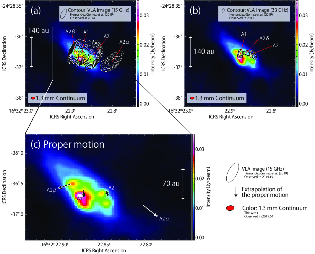


| Central Mass () | ||||||||
|---|---|---|---|---|---|---|---|---|
| Inclination Anglebb0° for a face-on configuration. (°) | 0.5 | 1.0 | 1.5 | 2.0 | 2.5 | 3.0 | 3.5 | 4.0 |
| 90 | 5.84 | 5.14 | 4.32 | 4.32 | 5.78 | 7.80 | 9.42 | 10.64 |
| 80 | 5.82 | 5.16 | 4.33 | 4.17 | 5.47 | 7.45 | 9.25 | 10.53 |
| 70 | 5.61 | 4.65 | 3.80 | 3.38 | 4.27 | 6.69 | 10.92 | 16.58 |
| 60 | 5.65 | 4.85 | 4.33 | 3.96 | 4.54 | 5.52 | 6.28 | 6.41 |
| 50 | 5.84 | 5.25 | 4.71 | 4.30 | 4.22 | 4.69 | 5.44 | 6.03 |
| 40 | 6.10 | 5.56 | 5.11 | 4.70 | 4.54 | 4.26 | 4.30 | 4.60 |
| 30 | 6.42 | 5.94 | 5.62 | 5.49 | 5.07 | 4.83 | 4.73 | 4.56 |
| Central Mass () | ||||||||||
|---|---|---|---|---|---|---|---|---|---|---|
| Inclination Anglebb0° for a face-on configuration. (°) | 0.2 | 0.4 | 0.6 | 0.8 | 1.0 | 1.2 | 1.4 | 1.6 | 1.8 | 2.0 |
| 90 | 5.77 | 4.45 | 3.15 | 2.37 | 2.24 | 2.67 | 3.51 | 4.90 | 6.72 | 8.78 |
| 80 | 5.79 | 4.49 | 3.19 | 2.36 | 2.18 | 2.55 | 3.34 | 4.67 | 6.42 | 8.41 |
| 70 | 5.73 | 4.77 | 3.85 | 3.24 | 3.02 | 3.39 | 4.16 | 5.25 | 10.59 | 16.56 |
| 60 | 5.91 | 5.25 | 4.60 | 4.11 | 3.85 | 4.12 | 4.82 | 5.85 | 7.19 | 8.81 |
| 50 | 6.09 | 5.55 | 5.10 | 4.71 | 4.36 | 4.12 | 4.17 | 4.51 | 4.98 | 5.56 |
| 40 | 6.30 | 5.83 | 5.51 | 5.20 | 4.86 | 4.58 | 4.40 | 4.20 | 4.13 | 4.25 |
| 30 | 6.48 | 6.24 | 5.88 | 5.66 | 5.46 | 5.21 | 4.96 | 4.83 | 4.62 | 4.47 |
| Central Mass () | ||||||||||
|---|---|---|---|---|---|---|---|---|---|---|
| Inclination Anglebb0° for a face-on configuration. (°) | 0.1 | 0.2 | 0.3 | 0.4 | 0.5 | 0.6 | 0.7 | 0.8 | 0.9 | 1.0 |
| 90 | 12.75 | 11.21 | 9.03 | 8.51 | 9.12 | 10.34 | 11.52 | 12.67 | 13.72 | 14.50 |
| 80 | 12.62 | 10.92 | 8.73 | 8.14 | 8.77 | 10.02 | 11.43 | 12.68 | 13.88 | 14.78 |
| 70 | 12.41 | 10.34 | 8.08 | 7.34 | 7.91 | 9.25 | 10.92 | 12.70 | 14.29 | 15.74 |
| 60 | 12.17 | 10.41 | 8.17 | 7.07 | 7.21 | 8.32 | 10.05 | 12.18 | 14.34 | 16.41 |
| 50 | 12.48 | 11.11 | 9.39 | 7.87 | 7.29 | 7.56 | 8.56 | 10.13 | 12.09 | 14.32 |
| 40 | 13.03 | 11.95 | 11.02 | 9.83 | 8.65 | 7.95 | 7.77 | 8.04 | 8.76 | 9.81 |
| 30 | 13.69 | 12.85 | 12.22 | 11.74 | 11.29 | 10.59 | 9.82 | 9.12 | 8.63 | 8.32 |
| 20 | 14.12 | 13.73 | 13.32 | 12.96 | 12.62 | 12.39 | 12.26 | 12.12 | 12.05 | 11.65 |
| 10 | 14.61 | 14.32 | 14.18 | 14.02 | 13.91 | 13.82 | 13.68 | 13.64 | 13.47 | 13.44 |
| Central Mass () | ||||||
|---|---|---|---|---|---|---|
| Radius of the CBbbThe radius of the centrifugal barrier. (au) | Inclination Anglecc0° for a face-on configuration. (°) | 0.10 | 0.15 | 0.20 | 0.25 | 0.30 |
| 5 | 90 | 14.49 | 12.92 | 12.46 | 13.59 | 15.94 |
| 80 | 13.50 | 11.85 | 11.56 | 12.64 | 14.90 | |
| 70 | 12.73 | 11.07 | 10.58 | 11.29 | 12.96 | |
| 60 | 12.95 | 11.30 | 10.51 | 10.76 | 11.73 | |
| 50 | 13.86 | 12.82 | 11.82 | 11.51 | 11.80 | |
| 10 | 90 | 12.86 | 10.95 | 10.40 | 11.53 | 13.77 |
| 80 | 12.31 | 10.22 | 9.62 | 10.55 | 12.53 | |
| 70 | 11.94 | 9.84 | 8.98 | 9.48 | 10.96 | |
| 60 | 12.50 | 10.75 | 9.44 | 9.37 | 10.19 | |
| 50 | 13.81 | 12.79 | 11.29 | 10.51 | 10.58 | |
| 20 | 90 | 13.15 | 11.22 | 9.80 | 10.04 | 11.76 |
| 80 | 13.06 | 11.35 | 9.84 | 9.99 | 11.54 | |
| 70 | 13.63 | 12.14 | 10.58 | 10.31 | 11.52 | |
| 60 | 14.63 | 13.85 | 12.33 | 11.55 | 11.91 | |
| 50 | 14.76 | 14.36 | 13.77 | 12.89 | 12.36 | |


