Substitute adjustment via recovery of latent variables

Jeffrey Adams^♯ [email protected] and Niels Richard Hansen^♯ [email protected] ^♯Department of Mathematical Sciences, University of Copenhagen
Universitetsparken 5, Copenhagen, 2100, Denmark

Abstract.

The deconfounder was proposed as a method for estimating causal parameters in a context with multiple causes and unobserved confounding. It is based on recovery of a latent variable from the observed causes. We disentangle the causal interpretation from the statistical estimation problem and show that the deconfounder in general estimates adjusted regression target parameters. It does so by outcome regression adjusted for the recovered latent variable termed the substitute. We refer to the general algorithm, stripped of causal assumptions, as substitute adjustment. We give theoretical results to support that substitute adjustment estimates adjusted regression parameters when the regressors are conditionally independent given the latent variable. We also introduce a variant of our substitute adjustment algorithm that estimates an assumption-lean target parameter with minimal model assumptions. We then give finite sample bounds and asymptotic results supporting substitute adjustment estimation in the case where the latent variable takes values in a finite set. A simulation study illustrates finite sample properties of substitute adjustment. Our results support that when the latent variable model of the regressors hold, substitute adjustment is a viable method for adjusted regression.

1. Introduction

The deconfounder was proposed by Wang & Blei (2019) as a general algorithm for estimating causal parameters via outcome regression when: (1) there are multiple observed causes of the outcome; (2) the causal effects are potentially confounded by a latent variable; (3) the causes are conditionally independent given a latent variable $Z$ . The proposal spurred discussion and criticism; see the comments to (Wang & Blei, 2019) and the contributions by D’Amour (2019); Ogburn et al. (2020) and Grimmer et al. (2023). One question raised was whether the assumptions made by Wang & Blei (2019) are sufficient to claim that the deconfounder estimates a causal parameter. Though an amendment by Wang & Blei (2020) addressed the criticism and clarified their assumptions, it did not resolve all questions regarding the deconfounder.

The key idea of the deconfounder is to recover the latent variable $Z$ from the observed causes and use this substitute confounder as a replacement for the unobserved confounder. The causal parameter is then estimated by outcome regression using the substitute confounder for adjustment. This way of adjusting for potential confounding has been in widespread use for some time in genetics and genomics, where, e.g., EIGENSTRAT based on PCA (Patterson et al., 2006; Price et al., 2006) was proposed to adjust for population structure in genome wide association studies (GWASs); see also (Song et al., 2015). Similarly, surrogate variable adjustment (Leek & Storey, 2007) adjusts for unobserved factors causing unwanted variation in gene expression measurements.

In our view, the discussion regarding the deconfounder was muddled by several issues. First, issues with non-identifiablity of target parameters from the observational distribution with a finite number of observed causes lead to confusion. Second, the causal role of the latent variable $Z$ and its causal relations to any unobserved confounder were difficult to grasp. Third, there was a lack of theory supporting that the deconfounder was actually estimating causal target parameters consistently. We defer the treatment of the thorny causal interpretation of the deconfounder to the discussion in Section 5 and focus here on the statistical aspects.

In our view, the statistical problem is best treated as adjusted regression without insisting on a causal interpretation. Suppose that we observe a real valued outcome variable $Y$ and additional variables $X_{1},X_{2},\ldots,X_{p}$ . We can then be interested in estimating the adjusted regression function

(1)

x\mapsto\mathbb{E}\left[\mathbb{E}\left[Y\mid X_{i}=x;\mathbf{X}_{-i}\right]\right]

where $\mathbf{X}_{-i}$ denotes all variables but $X_{i}$ . That is, we adjust for all other variables when regressing $Y$ on $X_{i}$ . The adjusted regression function could have a causal interpretation in some contexts, but it is also of interest without a causal interpretation. It can, for instance, be used to study the added predictive value of $X_{i}$ , and it is constant (as a function of $x$ ) if and only if $\mathbb{E}\left[Y\mid X_{i}=x;\mathbf{X}_{-i}\right]=\mathbb{E}\left[Y\mid\mathbf{X}_{-i}\right]$ ; that is, if and only if $Y$ is conditionally mean independent of $X_{i}$ given $\mathbf{X}_{-i}$ (Lundborg et al., 2023).

In the context of a GWAS, $Y$ is a continuous phenotype and $X_{i}$ represents a single nucleotide polymorphism (SNP) at the genomic site $i$ . The regression function (1) quantifies how much a SNP at site $i$ adds to the prediction of the phenotype outcome on top of all other SNP sites. In practice, only a fraction of all SNPs along the genome are observed, yet the number of SNPs can be in the millions, and estimation of the full regression model $\mathbb{E}\left[Y\mid X_{i}=x;\mathbf{X}_{-i}=\mathbf{x}_{-i}\right]$ can be impossible without model assumptions. Thus if the regression function (1) is the target of interest, it is extremely useful if we, by adjusting for a substitute of a latent variable, can obtain a computationally efficient and statistically valid estimator of (1).

From our perspective, when viewing the problem as that of adjusted regression, the most pertinent questions are: (1) when is adjustment by the latent variable $Z$ instead of $\mathbf{X}_{-i}$ appropriate; (2) can adjustment by substitutes of the latent variable, recovered from the observe $X_{i}$ -s, be justified; (3) can we establish an asymptotic theory that allows for statistical inference when adjusting for substitutes?

With the aim of answering the three questions above, this paper makes two main contributions:

A transparent statistical framework. We focus on estimation of the adjusted mean, thereby disentangling the statistical problem from the causal discussion. This way the target of inference is clear and so are the assumptions we need about the observational distribution in terms of the latent variable model. We present in Section 2 a general framework with an infinite number of $X_{i}$ -variables, and we present clear assumptions implying that we can replace adjustment by $\mathbf{X}_{-i}$ with adjustment by $Z$ . Within the general framework, we subsequently present an assumption-lean target parameter that is interpretable without restrictive model assumptions on the regression function.

A novel theoretical analysis. By restricting attention to the case where the latent variable $Z$ takes values in a finite set, we give in Section 3 bounds on the estimation error due to using substitutes and on the recovery error—that is, the substitute mislabeling rate. These bounds quantify, among other things, how the errors depend on $p$ ; the actual (finite) number of $X_{i}$ -s used for recovery. With minimal assumptions on the conditional distributions in the latent variable model and on the outcome model, we use our bounds to derive asymptotic conditions ensuring that the assumption-lean target parameter can be estimated just as well using substitutes as if the latent variables were observed.

To implement substitute adjustment in practice, we leverage recent developments on estimation in finite mixture models via tensor methods, which are computationally and statistically efficient in high dimensions. We illustrate our results via a simulation study in Section 4. Proofs and auxiliary results are in Appendix A. Appendix B contains a complete characterization of when recovery of $Z$ is possible from an infinite $\mathbf{X}$ in a Gaussian mixture model.

1.1. Relation to existing literature

Our framework and results are based on ideas by Wang & Blei (2019, 2020) and the literature preceding them on adjustment by surrogate/substitute variables. We add new results to this line of research on the theoretical justification of substitute adjustment as a method for estimation.

There is some literature on the theoretical properties of tests and estimators in high-dimensional problems with latent variables. Somewhat related to our framework is the work by Wang et al. (2017) on adjustment for latent confounders in multiple testing, motivated by applications to gene expression analysis. More directly related is the work by Ćevid et al. (2020) and Guo, Ćevid & Bühlmann (2022), who analyze estimators within a linear modelling framework with unobserved confounding. While their methods and results are definitely interesting, they differ from substitute adjustment, since they do not directly attempt to recover the latent variables. The linearity and sparsity assumptions, which we will not make, play an important role for their methods and analysis.

The paper by Grimmer et al. (2023) comes closest to our framework and analysis. Grimmer et al. (2023) present theoretical results and extensive numerical examples, primarily with a continuous latent variable. Their results are not favorable for the deconfounder and they conclude that the deconfounder is “not a viable substitute for careful research design in real-world applications”. Their theoretical analyses are mostly in terms of computing the population (or $n$ -asymptotic) bias of a method for a finite $p$ (the number of $X_{i}$ -variables), and then possibly investigate the limit of the bias as $p$ tends to infinity. Compared to this, we analyze the asymptotic behaviour of the estimator based on substitute adjustment as $n$ and $p$ tend to infinity jointly. Moreover, since we specifically treat discrete latent variables, some of our results are also in a different framework.

2. Substitute adjustment

2.1. The General Model

The full model is specified in terms of variables $(\mathbf{X},Y)$ , where $Y\in\mathbb{R}$ is a real valued outcome variable of interest and $\mathbf{X}\in\mathbb{R}^{\mathbb{N}}$ is a infinite vector of additional real valued variables. That is, $\mathbf{X}=(X_{i})_{i\in\mathbb{N}}$ with $X_{i}\in\mathbb{R}$ for $i\in\mathbb{N}$ . We let $\mathbf{X}_{-i}=(X_{j})_{j\in\mathbb{N}\backslash{\{i\}}}$ , and define (informally) for each $i\in\mathbb{N}$ and $x\in\mathbb{R}$ the target parameter of interest

(2)

\chi_{x}^{i}=\mathbb{E}\left[\mathbb{E}\left[Y\;\middle|\;X_{i}=x;\mathbf{X}_{-i}\right]\right].

That is, $\chi_{x}^{i}$ is the mean outcome given $X_{i}=x$ when adjusting for all remaining variables $\mathbf{X}_{-i}$ . Since $\mathbb{E}\left[Y\mid X_{i}=x;\mathbf{X}_{-i}\right]$ is generally not uniquely defined for all $x\in\mathbb{R}$ by the distribution of $(\mathbf{X},Y)$ , we need some additional structure to formally define $\chi^{i}_{x}$ . The following assumption and subsequent definition achieve this by assuming that a particular choice of the conditional expectation is made and remains fixed. Throughout, $\mathbb{R}$ is equipped with the Borel $\sigma$ -algebra and $\mathbb{R}^{\mathbb{N}}$ with the corresponding product $\sigma$ -algebra.

Assumption 1 (Regular Conditional Distribution).

Fix for each $i\in\mathbb{N}$ a Markov kernel $(P_{x,\mathbf{x}}^{i})_{(x,\mathbf{x})\in\mathbb{R}\times\mathbb{R}^{\mathbb{N}}}$ on $\mathbb{R}$ . Assume that $P_{x,\mathbf{x}}^{i}$ is the regular conditional distribution of $Y$ given $(X_{i},\mathbf{X}_{-i})=(x,\mathbf{x})$ for all $x\in\mathbb{R}$ , $\mathbf{x}\in\mathbb{R}^{\mathbb{N}}$ and $i\in\mathbb{N}$ . With $P^{-i}$ the distribution of $\mathbf{X}_{-i}$ , suppose additionally that

\iint|y|\,P^{i}_{x,\mathbf{x}}(\mathrm{d}y)P^{-i}(\mathrm{d}\mathbf{x})<\infty

for all $x\in\mathbb{R}$ .

Definition 1.

Under Assumption 1 we define

(3)

\chi_{x}^{i}=\iint y\,P^{i}_{x,\mathbf{x}}(\mathrm{d}y)P^{-i}(\mathrm{d}\mathbf{x}).

Remark 1.

Definition 1 makes the choice of conditional expectation explicit by letting

\mathbb{E}\left[Y\mid X_{i}=x;\mathbf{X}_{-i}\right]=\int y\,P^{i}_{x,\mathbf{X}_{-i}}(\mathrm{d}y)

be defined in terms of the specific regular conditional distribution that is fixed according to Assumption 1. We may need additional regularity assumptions to identify this Markov kernel from the distribution of $(\mathbf{X},Y)$ , which we will not pursue here.

The main assumption in this paper is the existence of a latent variable, $Z$ , that will render the $X_{i}$ -s conditionally independent, and which can be recovered from $\mathbf{X}$ in a suitable way. The variable $Z$ will take values in a measurable space $(E,\mathcal{E})$ , which we assume to be a Borel space. We use the notation $\sigma(Z)$ and $\sigma(\mathbf{X}_{-i})$ to denote the $\sigma$ -algebras generated by $Z$ and $\mathbf{X}_{-i}$ , respectively.

Assumption 2 (Latent Variable Model).

There is a random variable $Z$ with values in $(E,\mathcal{E})$ such that:

(1)

$X_{1},X_{2},\ldots$ are conditionally independent given $Z$ ,
(2)

$\sigma(Z)\subseteq\bigcap_{i=1}^{\infty}\sigma(\mathbf{X}_{-i})$ .

The latent variable model given by Assumption 2 allows us to identify the adjusted mean by adjusting for the latent variable only.

Proposition 1.

Fix $i\in\mathbb{N}$ and let $P^{-i}_{z}$ denote a regular conditional distribution of $\mathbf{X}_{-i}$ given $Z=z$ . Under Assumptions 1 and 2, the Markov kernel

(4)

Q_{x,z}^{i}(A)=\int P^{i}_{x,\mathbf{x}}(A)P^{-i}_{z}(\mathrm{d}\mathbf{x}),\qquad A\subseteq\mathbb{R}

is a regular conditional distribution of $Y$ given $(X_{i},Z)=(x,z)$ , in which case

(5)

\chi_{x}^{i}=\iint y\,Q_{x,z}^{i}(\mathrm{d}y)P^{Z}(\mathrm{d}z)=\mathbb{E}\left[\mathbb{E}\left[Y\mid X_{i}=x;Z\right]\right].

Figure 1. Directed Acyclic Graph (DAG) representing the joint distribution of

(X_{i},\mathbf{X}_{-i},Z,Y)

. The variable

Z

blocks the backdoor from

X_{i}

Y

The joint distribution of $(X_{i},\mathbf{X}_{-i},Z,Y)$ is, by Assumption 2, Markov w.r.t. to the graph in Figure 1. Proposition 1 is essentially the backdoor criterion, since $Z$ blocks the backdoor from $X_{i}$ to $Y$ via $\mathbf{X}_{-i}$ ; see Theorem 3.3.2 in (Pearl, 2009) or Proposition 6.41(ii) in (Peters et al., 2017). Nevertheless, we include a proof in Appendix A for two reasons. First, Proposition 1 does not involve causal assumptions about the model, and we want to clarify that the mathematical result is agnostic to such assumptions. Second, the proof we give of Proposition 1 does not require regularity assumptions, such as densities of the conditional distributions, but it relies subtly on Assumption 2(2).

Example 1.

Suppose $\mathbb{E}[|X_{i}|]\leq C$ for all $i$ and some finite constant $C$ , and assume, for simplicity, that $\mathbb{E}[X_{i}]=0$ . Let $\boldsymbol{\beta}=(\beta_{i})_{i\in\mathbb{N}}\in\ell_{1}$ and define

\langle\boldsymbol{\beta},\mathbf{X}\rangle=\sum_{i=1}^{\infty}\beta_{i}X_{i}.

The infinite sum converges almost surely since $\boldsymbol{\beta}\in\ell_{1}$ . With $\varepsilon$ being $\mathcal{N}(0,1)$ -distributed and independent of $\mathbf{X}$ consider the outcome model

Y=\langle\boldsymbol{\beta},\mathbf{X}\rangle+\varepsilon.

Letting $\boldsymbol{\beta}_{-i}$ denote the $\boldsymbol{\beta}$ -sequence with the $i$ -th coordinate removed, a straightforward, though slightly informal, computation, gives

	$\displaystyle\chi^{i}_{x}$	$\displaystyle=\mathbb{E}\left[\mathbb{E}\left[\beta_{i}X_{i}+\langle\boldsymbol{\beta}_{-i},\mathbf{X}_{-i}\rangle\mid X_{i}=x;\mathbf{X}_{-i}\right]\right]$
		$\displaystyle=\beta_{i}x+\mathbb{E}\left[\langle\boldsymbol{\beta}_{-i},\mathbf{X}_{-i}\rangle\right]=\beta_{i}x+\langle\boldsymbol{\beta}_{-i},\mathbb{E}\left[\mathbf{X}_{-i}\right]\rangle=\beta_{i}x.$

To fully justify the computation, via Assumption 1, we let $P^{i}_{x,\mathbf{x}}$ be the $\mathcal{N}(\beta_{i}x+\langle\boldsymbol{\beta}_{-i},\mathbf{x}\rangle,1)$ -distribution for the $P^{-i}$ -almost all $\mathbf{x}$ where $\langle\boldsymbol{\beta}_{-i},\mathbf{x}\rangle$ is well defined. For the remaining $\mathbf{x}$ we let $P^{i}_{x,\mathbf{x}}$ be the $\mathcal{N}(\beta_{i}x,1)$ -distribution. Then $P^{i}_{x,\mathbf{x}}$ is a regular conditional distribution of $Y$ given $(X_{i},\mathbf{X}_{-i})=(x,\mathbf{x})$ ,

\int y\,P_{x,\mathbf{x}}^{i}(\mathrm{d}y)=\beta_{i}x+\langle\boldsymbol{\beta}_{-i},\mathbf{x}\rangle\quad\text{for }P^{-i}\text{-almost all }\mathbf{x},

and $\chi^{i}_{x}=\beta_{i}x$ follows from (3). It also follows from (4) that for $P^{Z}$ -almost all $z\in E$ ,

	$\displaystyle\mathbb{E}\left[Y\mid X_{i}=x;Z=z\right]$	$\displaystyle=\int y\,Q^{i}_{x,z}(\mathrm{d}y)$
		$\displaystyle=\beta_{i}x+\int\langle\boldsymbol{\beta}_{-i},\mathbf{x}\rangle P^{-i}_{z}(\mathrm{d}\mathbf{x})$
		$\displaystyle=\beta_{i}x+\sum_{j\neq i}\beta_{j}\mathbb{E}[X_{j}\mid Z=z].$

That is, with $\Gamma_{-i}(z)=\sum_{j\neq i}\beta_{j}\mathbb{E}[X_{j}\mid Z=z]$ , the regression model

\mathbb{E}\left[Y\mid X_{i}=x;Z=z\right]=\beta_{i}x+\Gamma_{-i}(z)

is a partially linear model.

Example 2.

While Example 1 is explicit about the outcome model, it does not describe an explicit latent variable model fulfilling Assumption 2. To this end, take $E=\mathbb{R}$ , let $Z^{\prime},U_{1},U_{2},\ldots$ be i.i.d. $\mathcal{N}(0,1)$ -distributed and set $X_{i}=Z^{\prime}+U_{i}$ . By the Law of Large Numbers, for any $i\in\mathbb{N}$ ,

\frac{1}{n}\sum_{j=1;j\neq i}^{n+1}X_{j}=Z^{\prime}+\frac{1}{n}\sum_{j=1;j\neq i}^{n+1}U_{j}\rightarrow Z^{\prime}

almost surely for $n\to\infty$ . Setting

Z=\left\{\begin{array}[]{ll}\lim\limits_{n\to\infty}\frac{1}{n}\sum_{j=1;j\neq i}^{n+1}X_{j}&\quad\text{if the limit exists}\\ 0&\quad\text{otherwise}\end{array}\right.

we get that $\sigma(Z)\subseteq\sigma(\mathbf{X}_{-i})$ for any $i\in\mathbb{N}$ and $Z=Z^{\prime}$ almost surely. Thus, Assumption 2 holds.

Continuing with the outcome model from Example 1, we see that for $P^{Z}$ -almost all $z\in E$ ,

\mathbb{E}[X_{j}\mid Z=z]=\mathbb{E}[Z^{\prime}+U_{j}\mid Z=z]=z,

thus $\Gamma_{-i}(z)=\gamma_{-i}z$ with $\gamma_{-i}=\sum_{j\neq i}\beta_{j}$ . In this example it is actually possible to compute the regular conditional distribution, $Q^{i}_{x,z}$ , of $Y$ given $(X_{i},Z)=(x,z)$ explicitly. It is the $\mathcal{N}\left(\beta_{i}x+\gamma_{-i}z,1+\|\boldsymbol{\beta}_{-i}\|^{2}_{2}\right)$ -distribution where $\|\boldsymbol{\beta}_{-i}\|^{2}_{2}=\langle\boldsymbol{\beta}_{-i},\boldsymbol{\beta}_{-i}\rangle$ .

2.2. Substitute Latent Variable Adjustment

Proposition 1 tells us that under Assumptions 1 and 2 the adjusted mean, $\chi_{x}^{i}$ , defined by adjusting for the entire infinite vector $\mathbf{X}_{-i}$ , is also given by adjusting for the latent variable $Z$ . If the latent variable were observed we could estimate $\chi^{i}_{x}$ in terms of an estimate of the following regression function.

Definition 2 (Regression function).

Under Assumptions 1 and 2 define the regression function

(6)

b_{x}^{i}(z)=\int y\,Q_{x,z}^{i}(\mathrm{d}y)=\mathbb{E}\left[Y\mid X_{i}=x;Z=z\right]

where $Q_{x,z}^{i}$ is given by (4).

If we had $n$ i.i.d. observations, $(x_{i,1},z_{1},y_{1}),\ldots,(x_{i,n},z_{n},y_{n})$ , of $(X_{i},Z,Y)$ , a straightforward plug-in estimate of $\chi^{i}_{x}$ is

(7)

\hat{\chi}^{i}_{x}=\frac{1}{n}\sum_{k=1}^{n}\hat{b}_{x}^{i}(z_{k}),

where $\hat{b}_{x}^{i}(z)$ is an estimate of the regression function $b_{x}^{i}(z)$ . In practice we do not observe the latent variable $Z$ . Though Assumption 2(2) implies that $Z$ can be recovered from $\mathbf{X}$ , we do not assume we know this recovery map, nor do we in practice observe the entire $\mathbf{X}$ , but only the first $p$ coordinates, $\mathbf{X}_{1:p}=(X_{1},\ldots,X_{p})$ .

We thus need an estimate of a recovery map, $\hat{f}^{p}:\mathbb{R}^{p}\to E$ , such that for the substitute latent variable $\hat{Z}=\hat{f}^{p}(\mathbf{X}_{1:p})$ we have¹¹1We can in general only hope to learn a recovery map of $Z$ up to a Borel isomorphism, but this is also all that is needed, cf. Assumption 2. that $\sigma(\hat{Z})$ approximately contains the same information as $\sigma(Z)$ . Using such substitutes, a natural way to estimate $\chi^{i}_{x}$ is given by Algorithm 1, which is a general three-step procedure returning the estimate $\widehat{\chi}^{i,\mathrm{sub}}_{x}$ .

1 input: data

\mathcal{S}_{0}=\{\mathbf{x}_{1:p,1}^{0},\ldots,\mathbf{x}_{1:p,m}^{0}\}

and

\mathcal{S}=\{(\mathbf{x}_{1:p,1},y_{1}),\ldots(\mathbf{x}_{1:p,n},y_{n})\}

, a set

E

i\in\{1,\ldots,p\}

and

x\in\mathbb{R}

;

2 options: a method for estimating a recovery map

f^{p}:\mathbb{R}^{p}\to E

, a method for estimating the regression function

z\mapsto b_{x}^{i}(z)

;

3 begin

4 use data in

\mathcal{S}_{0}

to compute the estimate

\hat{f}^{p}

of the recovery map.

5 use data in

\mathcal{S}

to compute the substitute latent variables as

\hat{z}_{k}:=\hat{f}^{p}(\mathbf{x}_{1:p,k})

k=1,\ldots,n

6 use data in

\mathcal{S}

combined with the substitutes to compute the regression function estimate,

z\mapsto\hat{b}_{x}^{i}(z)

, and set

\widehat{\chi}^{i,\mathrm{sub}}_{x}=\frac{1}{n}\sum_{k=1}^{n}\hat{b}_{x}^{i}(\hat{z}_{k}).

7 end

return $\widehat{\chi}^{i,\mathrm{sub}}_{x}$

Algorithm 1 General Substitute Adjustment

The regression estimate $\hat{b}_{x}^{i}(z)$ in Algorithm 1 is computed on the basis of the substitutes, which likewise enter into the final computation of $\widehat{\chi}^{i,\mathrm{sub}}_{x}$ . Thus the estimate is directly estimating $\chi^{i,\mathrm{sub}}_{x}=\mathbb{E}\left[\mathbb{E}\left[Y\mid X_{i}=x;\hat{Z}\right]\;\middle|\;\hat{f}^{p}\right]$ , and it is expected to be biased as an estimate of $\chi^{i}_{x}$ . The general idea is that under some regularity assumptions, and for $p\to\infty$ and $m\to\infty$ appropriately, $\chi^{i,\mathrm{sub}}_{x}\to\chi^{i}_{x}$ and the bias vanishes asymptotically. Section 3 specifies a setup where such a result is shown rigorously.

Note that the estimated recovery map $\hat{f}^{p}$ in Algorithm 1 is the same for all $i=1,\ldots,p$ . Thus for any fixed $i$ , the $x_{i,k}^{0}$ -s are used for estimation of the recovery map, and the $x_{i,k}$ -s are used for the computation of the substitutes. Steps 4 and 5 of the algorithm could be changed to construct a recovery map $\hat{f}_{-i}^{p}$ independent of the $i$ -th coordinate. This appears to align better with Assumption 2, and it would most likely make the $\hat{z}_{k}$ -s slightly less correlated with the $x_{i,k}$ -s. It would, on the other hand, lead to a slightly larger recovery error, and worse, a substantial increase in the computational complexity if we want to estimate $\widehat{\chi}_{x}^{i,\mathrm{sub}}$ for all $i=1,\ldots,p$ .

Algorithm 1 leaves some options open. First, the estimation method used to compute $\hat{f}^{p}$ could be based on any method for estimating a recovery map, e.g., using a factor model if $E=\mathbb{R}$ or a mixture model if $E$ is finite. The idea of such methods is to compute a parsimonious $\hat{f}^{p}$ such that: (1) conditionally on $\hat{z}^{0}_{k}=\hat{f}^{p}(\mathbf{x}_{1:p,k}^{0})$ the observations $x_{1,k}^{0},\ldots,x_{p,k}^{0}$ are approximately independent for $k=1,\ldots,m$ ; and (2) $\hat{z}^{0}_{k}$ is minimally predictive of $x_{i,k}^{0}$ for $i=1,\ldots,p$ . Second, the regression method for estimation of the regression function $b_{x}^{i}(z)$ could be any parametric or nonparametric method. If $E=\mathbb{R}$ we could use OLS combined with the parametric model $b_{x}^{i}(z)=\beta_{0}+\beta_{i}x+\gamma_{-i}z$ , which would lead to the estimate

\widehat{\chi}^{i,\mathrm{sub}}_{x}=\hat{\beta}_{0}+\hat{\beta}_{i}x+\hat{\gamma}_{-i}\frac{1}{n}\sum_{k=1}^{n}\hat{z}_{k}.

If $E$ is finite, we could still use OLS but now combined with the parametric model $b_{x}^{i}(z)=\beta_{i,z}^{\prime}x+\gamma_{-i,z}$ , which would lead to the estimate

\widehat{\chi}^{i,\mathrm{sub}}_{x}=\left(\frac{1}{n}\sum_{k=1}^{n}\hat{\beta}_{i,\hat{z}_{k}}^{\prime}\right)x+\frac{1}{n}\sum_{k=1}^{n}\hat{\gamma}_{-i,\hat{z}_{k}}.

The relation between the two datasets in Algorithm 1 is not specified by the algorithm either. It is possible that they are independent, e.g., by data splitting, in which case $\hat{f}^{p}$ is independent of the data in $\mathcal{S}$ . It is also possible that $m=n$ and $\mathbf{x}_{1:p,k}^{0}=\mathbf{x}_{1:p,k}$ for $k=1,\ldots,n$ . While we will assume $\mathcal{S}_{0}$ and $\mathcal{S}$ independent for the theoretical analysis, the $\mathbf{x}_{1:p}$ -s from $\mathcal{S}$ will in practice often be part of $\mathcal{S}_{0}$ , if not all of $\mathcal{S}_{0}$ .

2.3. Assumption-Lean Substitute Adjustment

If the regression model in the general Algorithm 1 is misspecified we cannot expect that $\widehat{\chi}^{i,\mathrm{sub}}_{x}$ is a consistent estimate of $\chi^{i}_{x}$ . In Section 3 we investigate the distribution of a substitute adjustment estimator in the case where $E$ is finite. It is possible to carry out this investigation assuming a partially linear regression model, $b_{x}^{i}(z)=\beta_{i}x+\Gamma_{-i}(z)$ , but the results would then hinge on this model being correct. To circumvent such a model assumption we proceed instead in the spirit of assumption-lean regression (Berk et al., 2021; Vansteelandt & Dukes, 2022). Thus we focus on a univariate target parameter defined as a functional of the data distribution, and we then investigate its estimation via substitute adjustment.

Assumption 3 (Moments).

It holds that $\mathbb{E}(Y^{2})<\infty$ , $\mathbb{E}[X_{i}^{2}]<\infty$ and $\mathbb{E}\left[\operatorname{Var}\left[X_{i}\mid Z\right]\right]>0$ .

Definition 3 (Target parameter).

Let $i\in\mathbb{N}$ . Under Assumptions 2 and 3 define the target parameter

(8)

\beta_{i}=\frac{\operatorname{\mathbb{E}}\left[\operatorname{Cov}\left[X_{i},Y\mid Z\right]\right]}{\operatorname{\mathbb{E}}\left[\operatorname{Var}\left[X_{i}\mid Z\right]\right]}.

1 input: data

\mathcal{S}_{0}=\{\mathbf{x}_{1:p,1}^{0},\ldots,\mathbf{x}_{1:p,m}^{0}\}

and

\mathcal{S}=\{(\mathbf{x}_{1:p,1},y_{1}),\ldots(\mathbf{x}_{1:p,n},y_{n})\}

, a set

E

and

i\in\{1,\ldots,p\}

;

2 options: a method for estimating the recovery map

f^{p}:\mathbb{R}^{p}\to E

, methods for estimating the regression functions

\mu_{i}(z)=\mathbb{E}\left[X_{i}\mid Z=z\right]

and

g(z)=\mathbb{E}\left[Y\mid Z=z\right]

;

3 begin

4 use data in

\mathcal{S}_{0}

to compute the estimate

\hat{f}^{p}

of the recovery map.

5 use data in

\mathcal{S}

to compute the substitute latent variables as

\hat{z}_{k}:=\hat{f}^{p}(\mathbf{x}_{1:p,k})

k=1,\ldots,n

6 use data in

\mathcal{S}

combined with the substitutes to compute the regression function estimates

z\mapsto\hat{\mu}_{i}(z)

and

z\mapsto\hat{g}(z)

, and set

\widehat{\beta}^{\mathrm{sub}}_{i}=\frac{\sum_{k=1}^{n}(x_{i,k}-\hat{\mu}_{i}(\hat{z}_{k}))(y_{k}-\hat{g}(\hat{z}_{k}))}{\sum_{k=1}^{n}(x_{i,k}-\hat{\mu}_{i}(\hat{z}_{k}))^{2}}.

7 end

return $\widehat{\beta}^{\mathrm{sub}}_{i}$

Algorithm 2 Assumption-Lean Substitute Adjustment

Algorithm 2 gives a procedure for estimating $\beta_{i}$ based on substitute latent variables. The following proposition gives insight on the interpretation of the target parameter $\beta_{i}$ .

Proposition 2.

Under Assumptions 1, 2 and 3, and with $b_{x}^{i}(z)$ given as in Definition 2, and $\beta_{i}$ given as in Definition 3,

(9)

\beta_{i}=\frac{\operatorname{\mathbb{E}}\left[\operatorname{Cov}\left[X_{i},b^{i}_{X_{i}}(Z)\mid Z\right]\right]}{\operatorname{\mathbb{E}}\left[\operatorname{Var}\left[X_{i}\mid Z\right]\right]}.

Moreover, $\beta_{i}=0$ if $b^{i}_{x}(z)$ does not depend on $x$ . If $b^{i}_{x}(z)=\beta_{i}^{\prime}(z)x+\Gamma_{-i}(z)$ then

(10)

\beta_{i}=\mathbb{E}\left[w_{i}(Z)\beta_{i}^{\prime}(Z)\right]

where

w_{i}(Z)=\frac{\operatorname{Var}[X_{i}\mid Z]}{\mathbb{E}\left[\operatorname{Var}[X_{i}\mid Z]\right]}.

We include a proof of Proposition 2 in Appendix A.1 for completeness. The arguments are essentially as in (Vansteelandt & Dukes, 2022).

Remark 2.

If $b^{i}_{x}(z)=\beta_{i}^{\prime}(z)x+\Gamma_{-i}(z)$ it follows from Proposition 1 that $\chi^{i}_{x}=\beta^{\prime}_{i}x$ , where the coefficient $\beta^{\prime}_{i}=\mathbb{E}[\beta_{i}^{\prime}(Z)]$ may differ from $\beta_{i}$ given by (10). In the special case where the variance of $X_{i}$ given $Z$ is constant across all values of $Z$ , the weights in (10) are all $1$ , in which case $\beta_{i}=\beta^{\prime}_{i}$ . For the partially linear model, $b^{i}_{x}(z)=\beta_{i}^{\prime}x+\Gamma_{-i}(z)$ , with $\beta_{i}^{\prime}$ not depending on $z$ , it follows from (10) that $\beta_{i}=\beta_{i}^{\prime}$ irrespectively of the weights.

Remark 3.

If $X_{i}\in\{0,1\}$ then $b_{x}^{i}(z)=(b_{1}^{i}(Z)-b_{0}^{i}(Z))x+b_{0}^{i}(Z)$ , and the contrast $\chi^{i}_{1}-\chi^{i}_{0}=\mathbb{E}\left[b_{1}^{i}(Z)-b_{0}^{i}(Z)\right]$ is an unweighted mean of differences, while it follows from (10) that

(11)

\beta_{i}=\mathbb{E}\left[w_{i}(Z)(b_{1}^{i}(Z)-b_{0}^{i}(Z))\right].

If we let $\pi_{i}(Z)=\mathbb{P}(X_{i}=1\mid Z)$ , we see that the weights are given as

w_{i}(Z)=\frac{\pi_{i}(Z)(1-\pi_{i}(Z))}{\mathbb{E}\left[\pi_{i}(Z)(1-\pi_{i}(Z))\right]}.

We summarize three important take-away messages from Proposition 2 and the remarks above as follows:

Conditional mean independence:

The null hypothesis of conditional mean independence,

\mathbb{E}\left[Y\mid X_{i}=x;\mathbf{X}_{-i}\right])=\mathbb{E}\left[Y\mid\mathbf{X}_{-i}\right],

implies that $\beta_{i}=0$ . The target parameter $\beta_{i}$ thus suggests an assumption-lean approach to testing this null without a specific model of the conditional mean.

Heterogeneous partial linear model:

If the conditional mean,

b_{x}^{i}(z)=\mathbb{E}\left[Y\mid X_{i}=x;Z=z\right],

is linear in $x$ with an $x$ -coefficient that depends on $Z$ (heterogeneity), the target parameter $\beta_{i}$ is a weighted mean of these coefficients, while $\chi^{i}_{x}=\beta^{\prime}_{i}x$ with $\beta^{\prime}_{i}$ the unweighted mean.

Simple partial linear model:

If the conditional mean is linear in $x$ with an $x$ -coef-ficient that is independent of $Z$ (homogeneity), the target parameter $\beta_{i}$ coincides with this $x$ -coefficient and $\chi_{x}^{i}=\beta_{i}x$ . Example 1 is a special case where the latent variable model is arbitrary but the full outcome model is linear.

Just as for the general Algorithm 1, the estimate that Algorithm 2 outputs, $\widehat{\beta}^{\mathrm{sub}}_{i}$ , is not directly estimating the target parameter $\beta_{i}$ . It is directly estimating

(12)

\beta^{\mathrm{sub}}_{i}=\frac{\operatorname{\mathbb{E}}\left[\operatorname{Cov}\left[X_{i},Y\mid\hat{Z}\right]\;\middle|\;\hat{f}^{p}\right]}{\operatorname{\mathbb{E}}\left[\operatorname{Var}\left[X_{i}\mid\hat{Z}\right]\;\middle|\;\hat{f}^{p}\right]}.

Fixing the estimated recovery map $\hat{f}^{p}$ and letting $n\to\infty$ , we can expect that $\widehat{\beta}^{\mathrm{sub}}_{i}$ is consistent for $\beta^{\mathrm{sub}}_{i}$ and not for $\beta_{i}$ .

Pretending that the $z_{k}$ -s were observed, we introduce the oracle estimator

\widehat{\beta}_{i}=\frac{\sum_{k=1}^{n}(x_{i,k}-\overline{\mu}_{i}(z_{k}))(y_{k}-\overline{g}(z_{k}))}{\sum_{k=1}^{n}(x_{i,k}-\overline{\mu}_{i}(z_{k}))^{2}}.

Here, $\overline{\mu}_{i}$ and $\overline{g}$ denote estimates of the regression functions $\mu_{i}$ and $g$ , respectively, using the $z_{k}$ -s instead of the substitutes. The estimator $\widehat{\beta}_{i}$ is independent of $m$ , $p$ , and $\hat{f}^{p}$ , and when $(x_{i,1},z_{1},y_{1}),\ldots,(x_{i,n},z_{n},y_{n})$ are i.i.d. observations, standard regularity assumptions (van der Vaart, 1998) will ensure that the estimator $\widehat{\beta}_{i}$ is consistent for $\beta_{i}$ (and possibly even $\sqrt{n}$ -rate asymptotically normal). Writing

(13)

\widehat{\beta}^{\mathrm{sub}}_{i}-\beta_{i}=(\widehat{\beta}^{\mathrm{sub}}_{i}-\widehat{\beta}_{i})+(\hat{\beta}_{i}-\beta_{i})

we see that if we can appropriately bound the error, $|\widehat{\beta}^{\mathrm{sub}}_{i}-\widehat{\beta}_{i}|$ , due to using the substitutes instead of the unobserved $z_{k}$ -s, we can transfer asymptotic properties of $\hat{\beta}_{i}$ to $\widehat{\beta}^{\mathrm{sub}}_{i}$ . It is the objective of the following section to demonstrate how such a bound can be achieved for a particular model class.

3. Substitute adjustment in a mixture model

In this section, we present a theoretical analysis of assumption-lean substitute adjustment in the case where the latent variable takes values in a finite set. We provide finite-sample bounds on the error of $\widehat{\beta}^{\mathrm{sub}}_{i}$ due to the use of substitutes, and we show, in particular, that there exist trajectories of $m$ , $n$ and $p$ along which the estimator is asymptotically equivalent to the oracle estimator $\widehat{\beta}_{i}$ , which uses the actual latent variables.

3.1. The mixture model

To be concrete, we assume that $\mathbf{X}$ is generated by a finite mixture model such that conditionally on a latent variable $Z$ with values in a finite set, the coordinates of $\mathbf{X}$ are independent. The precise model specification is as follows.

Assumption 4 (Mixture Model).

There is a latent variable $Z$ with values in the finite set $E=\{1,\ldots,K\}$ such that $X_{1},X_{2},\ldots$ are conditionally independent given $Z=z$ . Furthermore,

(1)

The conditional distribution of $X_{i}$ given $Z=z$ has finite second moment, and its conditional mean and variance are denoted

	$\displaystyle\mu_{i}(z)$	$\displaystyle=\mathbb{E}[X_{i}\mid Z=z]$
	$\displaystyle\sigma_{i}^{2}(z)$	$\displaystyle=\operatorname{Var}[X_{i}\mid Z=z]$

for $z\in E$ and $i\in\mathbb{N}$ .

(2)

The conditional means satisfy the following separation condition

(14) $\sum_{i=1}^{\infty}(\mu_{i}(z)-\mu_{i}(v))^{2}=\infty$

for all $z,v\in E$ with $v\neq z$ .
(3)

There are constants $0<\sigma_{\min}^{2}\leq\sigma^{2}_{\max}<\infty$ that bound the conditional variances;

(15) $\sigma_{\min}^{2}\leq\max_{z\in E}\sigma_{i}^{2}(z)\leq\sigma^{2}_{\max}$

for all $i\in\mathbb{N}$ .
(4)

$\mathbb{P}(Z=z)>0$ for all $z\in E$ .

Algorithm 3 is one specific version of Algorithm 2 for computing $\hat{\beta}_{i}^{\mathrm{sub}}$ when the latent variable takes values in a finite set $E$ . The recovery map in Step 5 is given by computing the nearest mean, and it is thus estimated in Step 4 by estimating the means for each of the mixture components. How this is done precisely is an option of the algorithm. Once the substitutes are computed, outcome means and $x_{i,k}$ -means are (re)computed within each component. The computations in Steps 6 and 7 of Algorithm 3 result in the same estimator as the OLS estimator of $\beta_{i}$ when it is computed using the linear model

b_{x}^{i}(z)=\beta_{i}x+\gamma_{-i,z},\qquad\beta_{i},\gamma_{-i,1},\ldots,\gamma_{-i,K}\in\mathbb{R}

on the data $(x_{i,1},\hat{z}_{1},y_{1}),\ldots(x_{i,n},\hat{z}_{n},y_{n})$ . This may be relevant in practice, but it is also used in the proof of Theorem 1. The corresponding oracle estimator, $\hat{\beta}_{i}$ , is similarly an OLS estimator.

1 input: data

\mathcal{S}_{0}=\{\mathbf{x}_{1:p,1}^{0},\ldots,\mathbf{x}_{1:p,m}^{0}\}

and

\mathcal{S}=\{(\mathbf{x}_{1:p,1},y_{1}),\ldots(\mathbf{x}_{1:p,n},y_{n})\}

, a finite set

E

and

i\in\{1,\ldots,p\}

;

2 options: a method for estimating the conditional means

\mu_{j}(z)=\mathbb{E}[X_{j}\mid Z=z]

;

3 begin

4 use the data in

\mathcal{S}_{0}

to compute the estimates

\check{\mu}_{j}(z)

for

j\in\{1,\ldots,p\}

and

z\in E

5 use the data in

\mathcal{S}

to compute the substitute latent variables as

\hat{z}_{k}=\operatorname*{arg\,min}_{z}\|\mathbf{x}_{1:p,k}-\check{\boldsymbol{\mu}}_{1:p}(z)\|_{2}

k=1,\ldots,n

6 use the data in

\mathcal{S}

combined with the substitutes to compute the estimates

	$\displaystyle\hat{g}(z)$	$\displaystyle=\frac{1}{\hat{n}(z)}\sum_{k:\hat{z}_{k}=z}y_{k},\quad z\in E$
	$\displaystyle\hat{\mu}_{i}(z)$	$\displaystyle=\frac{1}{\hat{n}(z)}\sum_{k:\hat{z}_{k}=z}x_{i,k},\quad z\in E,$

where

\hat{n}(z)=\sum_{k=1}^{n}1(\hat{z}_{k}=z)

is the number of

k

-s with

\hat{z}_{k}=z

7 use the data in

\mathcal{S}

combined with the substitutes to compute

\widehat{\beta}^{\mathrm{sub}}_{i}=\frac{\sum_{k=1}^{n}(x_{i,k}-\hat{\mu}_{i}(\hat{z}_{k}))(y_{k}-\hat{g}(\hat{z}_{k}))}{\sum_{k=1}^{n}(x_{i,k}-\hat{\mu}_{i}(\hat{z}_{k}))^{2}}.

8 end

return $\widehat{\beta}^{\mathrm{sub}}_{i}$

Algorithm 3 Assumption Lean Substitute Adjustment w. Mixtures

Note that Assumption 4 implies that

	$\displaystyle\mathbb{E}[X_{i}^{2}]$	$\displaystyle=\sum_{z\in E}\mathbb{E}[X_{i}^{2}\mid Z=z]\mathbb{P}(Z=z)=\sum_{z\in E}(\sigma_{i}^{2}(z)+\mu_{i}(z)^{2})\mathbb{P}(Z=z)<\infty$
	$\displaystyle\mathbb{E}\left[\operatorname{Var}\left[X_{i}\mid Z\right]\right]$	$\displaystyle=\sum_{z\in E}\sigma_{i}^{2}(z)\mathbb{P}(Z=z)\geq\sigma_{\min}^{2}\min_{z\in E}\mathbb{P}(Z=z)>0.$

Hence Assumption 4, combined with $\mathbb{E}[Y^{2}]<\infty$ , ensure that the moment conditions in Assumption 3 hold.

The following proposition states that the mixture model given by Assumption 4 is a special case of the general latent variable model.

Proposition 3.

Assumption 4 on the mixture model implies Assumption 2. Specifically, that $\sigma(Z)\subseteq\sigma(\mathbf{X}_{-i})$ for all $i\in\mathbb{N}$ .

Remark 4.

The proof of Proposition 3 is in Appendix A.3. Technically, the proof only gives almost sure recovery of $Z$ from $\mathbf{X}_{-i}$ , and we can thus only conclude that $\sigma(Z)$ is contained in $\sigma(\mathbf{X}_{-i})$ up to negligible sets. We can, however, replace $Z$ by a variable, $Z^{\prime}$ , such that $\sigma(Z^{\prime})\subseteq\sigma(\mathbf{X}_{-i})$ and $Z^{\prime}=Z$ almost surely. We can thus simply swap $Z$ with $Z^{\prime}$ in Assumption 4.

Remark 5.

The arguments leading to Proposition 3 rely on Assumptions 4(2) and 4(3)—specifically the separation condition (14) and the upper bound in (15). However, these conditions are not necessary to be able to recover $Z$ from $\mathbf{X}_{-i}$ . Using Kakutani’s theorem on equivalence of product measures it is possible to characterize precisely when $Z$ can be recovered, but the abstract characterization is not particularly operational. In Appendix B we analyze the characterization for the Gaussian mixture model, where $X_{i}$ given $Z=z$ has a $\mathcal{N}(\mu_{i}(z),\sigma^{2}_{i}(z))$ -distribution. This leads to Proposition 5 and Corollary 1 in Appendix B, which gives necessary and sufficient conditions for recovery in the Gaussian mixture model.

3.2. Bounding estimation error due to using substitutes

In this section we derive an upper bound on the estimation error, which is due to using substitutes, cf. the decomposition (13). To this end, we consider the (partly hypothetical) observations $(x_{i,1},\hat{z}_{1},z_{1},y_{1}),\ldots(x_{i,n},\hat{z}_{n},z_{n},y_{n})$ , which include the otherwise unobserved $z_{k}$ -s as well as their observed substitutes, the $\hat{z}_{k}$ -s. We let $\mathbf{x}_{i}=(x_{i,1},\ldots,x_{i,n})^{T}\in\mathbb{R}^{n}$ and $\mathbf{y}=(y_{1},\ldots,y_{n})^{T}\in\mathbb{R}^{n}$ , and $\|\mathbf{x}_{i}\|_{2}$ and $\|\mathbf{y}\|_{2}$ denote the $2$ -norms of $\mathbf{x}_{i}$ and $\mathbf{y}$ , respectively. We also let

n(z)=\sum_{k=1}^{n}1(z_{k}=z)\qquad\text{and}\qquad\hat{n}(z)=\sum_{k=1}^{n}1(\hat{z}_{k}=z)

for $z\in E=\{1,\ldots,K\}$ , and

n_{\min}=\min\{n(1),\ldots,n(K),\hat{n}(1),\ldots,\hat{n}(K)\}.

Furthermore,

\overline{\mu}_{i}(z)=\frac{1}{n(z)}\sum_{k:z_{k}=z}x_{i,k},

and we define the following three quantities

(16)	$\displaystyle\alpha$	$\displaystyle=\frac{n_{\min}}{n}$
(17)	$\displaystyle\delta$	$\displaystyle=\frac{1}{n}\sum_{k=1}^{n}1(\hat{z}_{k}\neq z_{k})$
(18)	$\displaystyle\rho$	$\displaystyle=\frac{\min\left\{\sum_{k=1}^{n}(x_{i,k}-\overline{\mu}_{i}(z_{k}))^{2},\sum_{k=1}^{n}(x_{i,k}-\hat{\mu}_{i}(\hat{z}_{k}))^{2}\right\}}{\\|\mathbf{x}_{i}\\|_{2}^{2}}.$

Theorem 1.

Let $\alpha$ , $\delta$ and $\rho$ be given by (16), (17) and (18). If $\alpha,\rho>0$ then

(19)

|\widehat{\beta}^{\mathrm{sub}}_{i}-\hat{\beta}_{i}|\leq\frac{2\sqrt{2}}{\rho^{2}}\sqrt{\frac{\delta}{\alpha}}\frac{\|\mathbf{y}\|_{2}}{\|\mathbf{x}_{i}\|_{2}}.

The proof of Theorem 1 is given in Appendix A.2. Appealing to the Law of Large Numbers, the quantities in the upper bound (19) can be interpreted as follows:

•

The ratio $\|\mathbf{y}\|_{2}/\|\mathbf{x}_{i}\|_{2}$ is approximately a fixed and finite constant (unless $X_{i}$ is constantly zero) depending on the marginal distributions of $X_{i}$ and $Y$ only.
•

The fraction $\alpha$ is approximately

(20) $\min_{z\in E}\left\{\min\{\mathbb{P}(Z=z),\mathbb{P}(\hat{Z}=z)\}\right\},$

which is strictly positive by Assumption 4(4) (unless recovery is working poorly).

•

The quantity $\rho$ is a standardized measure of the residual variation of the $x_{i,k}$ -s within the groups defined by the $z_{k}$ -s or the $\hat{z}_{k}$ -s. It is approximately equal to the constant

\frac{\min\left\{\mathbb{E}\left[\operatorname{Var}\left[X_{i}\mid Z\right]\right],\mathbb{E}\left[\operatorname{Var}\left[X_{i}\mid\hat{Z}\right]\right]\right\}}{E(X_{i}^{2})},

which is strictly positive if the probabilities in (20) are strictly positive and not all of the conditional variances are $0$ .

•

The fraction $\delta$ is the relative mislabeling frequency of the substitutes. It is approximately equal to the mislabeling rate $\mathbb{P}(\hat{Z}\neq Z)$ .

The bound (19) tells us that if the mislabeling rate of the substitutes tends to $0$ , that is, if $\mathbb{P}(\hat{Z}\neq Z)\to 0$ , the estimation error tends to $0$ roughly like $\sqrt{\mathbb{P}(\hat{Z}\neq Z)}$ . This could potentially be achieved by letting $p\to\infty$ and $m\to\infty$ . We formalize this statement in Section 3.4.

3.3. Bounding the mislabeling rate of the substitutes

In this section we give bounds on the mislabeling rate, $\mathbb{P}(\hat{Z}\neq Z)$ , with the ultimate purpose of controlling the magnitude of $\delta$ in the bound (19). Two different approximations are the culprits of mislabeling. First, the computation of $\hat{Z}$ is based on the $p$ variables in $\mathbf{X}_{1:p}$ only, and it is thus an approximation of the full recovery map based on all variables in $\mathbf{X}$ . Second, the recovery map is an estimate and thus itself an approximation. The severity of the second approximation is quantified by the following relative errors of the conditional means used for recovery.

Definition 4 (Relative errors, $p$ -separation).

For the mixture model given by Assumption 4 let $\boldsymbol{\mu}_{1:p}(z)=(\mu_{i}(z))_{i=1,\ldots,p}\in\mathbb{R}^{p}$ for $z\in E$ . With $\check{\boldsymbol{\mu}}_{1:p}(z)\in\mathbb{R}^{p}$ for $z\in E$ any collection of $p$ -vectors, define the relative errors

(21)

R_{z,v}^{(p)}=\frac{\|\boldsymbol{\mu}_{1:p}(z)-\check{\boldsymbol{\mu}}_{1:p}(z)\|_{2}}{\|\boldsymbol{\mu}_{1:p}(z)-\boldsymbol{\mu}_{1:p}(v)\|_{2}}

for $z,v\in E$ , $v\neq z$ . Define, moreover, the minimal $p$ -separation as

(22)

\mathrm{sep}(p)=\min_{z\neq v}\norm{\boldsymbol{\mu}_{1:p}(z)-\boldsymbol{\mu}_{1:p}(v)}_{2}^{2}.

Note that Assumption 4(2) implies that $\mathrm{sep}(p)\to\infty$ for $p\to\infty$ . This convergence could be arbitrarily slow. The following definition captures the important case where the separation grows at least linearly in $p$ .

Definition 5 (Strong separation).

We say that the mixture model satisfies strong separation if there exists an $\varepsilon>0$ such that $\mathrm{sep}(p)\geq\varepsilon p$ eventually.

Strong separation is equivalent to

\liminf_{p\to\infty}\frac{\mathrm{sep}(p)}{p}>0.

A sufficient condition for strong separation is that $|\mu_{i}(z)-\mu_{i}(v)|\geq\varepsilon$ eventually for all $z,v\in E$ , $v\neq z$ and some $\varepsilon>0$ . That is, $\liminf_{i\to\infty}|\mu_{i}(z)-\mu_{i}(v)|>0$ for $v\neq z$ . When we have strong separation, then for $p$ large enough

\left(R_{z,v}^{(p)}\right)^{2}\leq\frac{1}{\varepsilon p}\|\boldsymbol{\mu}_{1:p}(z)-\check{\boldsymbol{\mu}}_{1:p}(z)\|_{2}^{2}\leq\frac{1}{\varepsilon}\max_{i=1,\ldots,p}\left(\mu_{i}(z)-\check{\mu}_{i}(z)\right)^{2},

and we note that it is conceivable²²2Parametric assumptions, say, and marginal estimators of each $\mu_{i}(z)$ that, under Assumption 4, are uniformly consistent over $i\in\mathbb{N}$ can be combined with a simple union bound to show the claim, possibly in a suboptimal way, cf. Section 3.5. that we can estimate $\boldsymbol{\mu}_{1:p}(z)$ by an estimator, $\check{\boldsymbol{\mu}}_{1:p}(z)$ , such that for $m,p\to\infty$ appropriately, $R_{z,v}^{(p)}\overset{P}{\to}0$ .

The following proposition shows that a bound on $R_{z,v}^{(p)}$ is sufficient to ensure that the growth of $\mathrm{sep}(p)$ controls how fast the mislabeling rate diminishes with $p$ . The proposition is stated for a fixed $\check{\boldsymbol{\mu}}$ , which means that when $\check{\boldsymbol{\mu}}$ is an estimate, we are effectively assuming it is independent of the template observation $(\mathbf{X}_{1:p},Z)$ used to compute $\hat{Z}$ .

Proposition 4.

Suppose that Assumption 4 holds. Let $\check{\boldsymbol{\mu}}_{1:p}(z)\in\mathbb{R}^{p}$ for $z\in E$ and let

\hat{Z}=\operatorname*{arg\,min}_{z}\|\mathbf{X}_{1:p}-\check{\boldsymbol{\mu}}_{1:p}(z)\|_{2}.

Suppose also that $R_{z,v}^{(p)}\leq\frac{1}{10}$ for all $z,v\in E$ with $v\neq z$ . Then

(23)

\mathbb{P}\left(\hat{Z}\neq Z\right)\leq\frac{25K\sigma^{2}_{\max}}{\mathrm{sep}(p)}.

If, in addition, the conditional distribution of $X_{i}$ given $Z=z$ is sub-Gaussian with variance factor $v_{\max}$ , independent of $i$ and $z$ , then

(24)

\mathbb{P}\left(\hat{Z}\neq Z\right)\leq K\exp\left(-\frac{\mathrm{sep}(p)}{50v_{\max}}\right)

Remark 6.

The proof of Proposition 4 is in Appendix A.3. It shows that the specific constants, $25$ and $50$ , appearing in the bounds above hinge on the specific bound, $R_{z,v}^{(p)}\leq\frac{1}{10}$ , on the relative error. The proof works for any bound strictly smaller than $\frac{1}{4}$ . Replacing $\frac{1}{10}$ by a smaller bound on the relative errors decreases the constant, but it will always be larger than $4$ .

The upshot of Proposition 4 is that if the relative errors, $R_{z,v}^{(p)}$ , are sufficiently small then Assumption 4 is sufficient to ensure that $\mathbb{P}\left(\hat{Z}\neq Z\right)\to 0$ for $p\to\infty$ . Without additional distributional assumptions the general bound (23) decays slowly with $p$ , and even with strong separation, the bound only gives a rate of $\tfrac{1}{p}$ . With the additional sub-Gaussian assumption, the rate is improved dramatically, and with strong separation it improves to $e^{-cp}$ for some constant $c>0$ . If the $X_{i}$ -s are bounded, their (conditional) distributions are sub-Gaussian, thus the rate is fast in this special but important case.

3.4. Asymptotics of the substitute adjustment estimator

Suppose $Z$ takes values in $E=\{1,\ldots,K\}$ and that $(x_{i,1},z_{1},y_{1}),\ldots,(x_{i,n},z_{n},y_{n})$ are observations of $(X_{i},Z,Y)$ . Then Assumption 3 ensures that the oracle OLS estimator $\widehat{\beta}_{i}$ is $\sqrt{n}$ -consistent and that

\widehat{\beta}_{i}\overset{\text{as}}{\sim}\mathcal{N}(\beta_{i},w_{i}^{2}/n).

There are standard sandwich formulas for the asymptotic variance parameter $w_{i}^{2}$ . In this section we combine the bounds from Sections 3.2 and 3.3 to show our main theoretical result; that $\widehat{\beta}^{\mathrm{sub}}_{i}$ is a consistent and asymptotically normal estimator of $\beta_{i}$ for $n,m\to\infty$ if also $p\to\infty$ appropriately.

Assumption 5.

The dataset $\mathcal{S}_{0}$ in Algorithm 3 consists of i.i.d. observations of $\mathbf{X}_{1:p}$ , the dataset $\mathcal{S}$ in Algorithm 3 consists of i.i.d. observations of $(\mathbf{X}_{1:p},Y)$ , and $\mathcal{S}$ is independent of $\mathcal{S}_{0}$ .

Theorem 2.

Suppose Assumption 1 holds and $E(Y^{2})<\infty$ , and consider the mixture model fulfilling Assumption 4. Consider data satisfying Assumption 5 and the estimator $\widehat{\beta}^{\mathrm{sub}}_{i}$ given by Algorithm 3. Suppose that $n,m,p\to\infty$ such that $\mathbb{P}(R_{z,v}^{(p)}>\tfrac{1}{10})\to 0$ . Then the following hold:

(1)

The estimation error due to using substitutes tends to $0$ in probability, that is,

$|\widehat{\beta}^{\mathrm{sub}}_{i}-\hat{\beta}_{i}|\overset{P}{\to}0,$

and $\widehat{\beta}^{\mathrm{sub}}_{i}$ is a consistent estimator of $\beta_{i}$ .
(2)

If $\frac{\mathrm{sep}(p)}{n}\to\infty$ and $n\mathbb{P}(R_{z,v}^{(p)}>\tfrac{1}{10})\to 0$ , then $\sqrt{n}|\widehat{\beta}^{\mathrm{sub}}_{i}-\hat{\beta}_{i}|\overset{P}{\to}0$ .
(3)

If $X_{i}$ conditionally on $Z=z$ is sub-Gaussian, with variance factor independent of $i$ and $z$ , and if $\frac{\mathrm{sep}(p)}{\log(n)}\to\infty$ and $n\mathbb{P}(R_{z,v}^{(p)}>\tfrac{1}{10})\to 0$ , then $\sqrt{n}|\widehat{\beta}^{\mathrm{sub}}_{i}-\hat{\beta}_{i}|\overset{P}{\to}0$ .

In addition, in case (2) as well as case (3), $\widehat{\beta}^{\mathrm{sub}}_{i}\overset{\text{as}}{\sim}\mathcal{N}(\beta_{i},w_{i}^{2}/n)$ , where the asymptotic variance parameter $w_{i}^{2}$ is the same as for the oracle estimator $\widehat{\beta}_{i}$ .

Remark 7.

The proof of Theorem 2 is in Appendix A.4. As mentioned in Remark 6, the precise value of the constant $\tfrac{1}{10}$ is not important. It could be replaced by any other constant strictly smaller than $\tfrac{1}{4}$ , and the conclusion would be the same.

Remark 8.

The general growth condition on $p$ in terms of $n$ in case (2) is bad; even with strong separation we would need $\tfrac{p}{n}\to\infty$ , that is, $p$ should grow faster than $n$ . In the sub-Gaussian case this improves substantially so that $p$ only needs to grow faster than $\log(n)$ .

3.5. Tensor decompositions

One open question from both a theoretical and practical perspective is how we construct the estimators $\check{\boldsymbol{\mu}}_{1:p}(z)$ . We want to ensure consistency for $m,p\to\infty$ , which is expressed as $\mathbb{P}\left(R_{z,v}^{(p)}>\tfrac{1}{10}\right)\to 0$ in our theoretical results, and that the estimator can be computed efficiently for large $m$ and $p$ . We indicated in Section 3.3 that simple marginal estimators of $\mu_{i}(z)$ can achieve this, but such estimators may be highly inefficient. In this section we briefly describe two methods based on tensor decompositions (Anandkumar et al., 2014) related to the third order moments of $\mathbf{X}_{1:p}$ . Thus to apply such methods we need to additionally assume that the $X_{i}$ -s have finite third moments.

Introduce first the third order $p\times p\times p$ tensor $G^{(p)}$ as

G^{(p)}=\sum_{i=1}^{p}\mathbf{a}_{i}\otimes\mathbf{e}_{i}\otimes\mathbf{e}_{i}+\mathbf{e}_{i}\otimes\mathbf{a}_{i}\otimes\mathbf{e}_{i}+\mathbf{e}_{i}\otimes\mathbf{e}_{i}\otimes\mathbf{a}_{i},

where $\mathbf{e}_{i}\in\mathbb{R}^{p}$ is the standard basis vector with a $1$ in the $i$ -th coordinate and $0$ elsewhere, and where

\mathbf{a}_{i}=\sum_{z\in E}\mathbb{P}(Z=z)\sigma_{i}^{2}(z)\boldsymbol{\mu}_{1:p}(z).

In terms of the third order raw moment tensor and $G^{(p)}$ we define the tensor

(25)

M_{3}^{(p)}=\mathbb{E}[\mathbf{X}_{1:p}\otimes\mathbf{X}_{1:p}\otimes\mathbf{X}_{1:p}]-G^{(p)}.

Letting $\mathcal{I}=\{(i_{1},i_{2},i_{3})\in\{1,\ldots,p\}\mid i_{1},i_{2},i_{3}\text{ all distinct}\}$ denote the set of indices of the tensors with all entries distinct, we see from the definition of $G^{(p)}$ that $G^{(p)}_{i_{1},i_{2},i_{3}}=0$ for $(i_{1},i_{2},i_{3})\in\mathcal{I}$ . Thus

(M_{3}^{(p)})_{i_{1},i_{2},i_{3}}=\mathbb{E}\left[X_{i_{1}}X_{i_{2}}X_{i_{3}}\right]

for $(i_{1},i_{2},i_{3})\in\mathcal{I}$ . In the following, $(M^{(p)}_{3})_{\mathcal{I}}$ denotes the incomplete tensor obtained by restricting the indices of $M^{(p)}_{3}$ to $\mathcal{I}$ .

The key to using the $M_{3}^{(p)}$ -tensor for estimation of the $\mu_{i}(z)$ -s is the following rank- $K$ tensor decomposition,

(26)

M_{3}^{(p)}=\sum_{z=1}^{K}\mathbb{P}(Z=z)\boldsymbol{\mu}_{1:p}(z)\otimes\boldsymbol{\mu}_{1:p}(z)\otimes\boldsymbol{\mu}_{1:p}(z);

see Theorem 3.3 in (Anandkumar et al., 2014) or the derivations on page 2 in (Guo, Nie & Yang, 2022).

Guo, Nie & Yang (2022) propose an algorithm based on incomplete tensor decomposition as follows: Let $(\widehat{M}_{3}^{(p)})_{\mathcal{I}}$ denote an estimate of the incomplete tensor $(M_{3}^{(p)})_{\mathcal{I}}$ ; obtain an approximate rank- $K$ tensor decomposition of the incomplete tensor $(\widehat{M}_{3}^{(p)})_{\mathcal{I}}$ ; extract estimates $\check{\boldsymbol{\mu}}_{1:p}(1),\ldots,\check{\boldsymbol{\mu}}_{1:p}(K)$ from this tensor decomposition. Theorem 4.2 in (Guo, Nie & Yang, 2022) shows that if the vectors $\boldsymbol{\mu}_{1:p}(1),\ldots,\boldsymbol{\mu}_{1:p}(K)$ satisfy certain regularity assumptions, they are estimated consistently by their algorithm (up to permutation) if $(\widehat{M}_{3}^{(p)})_{\mathcal{I}}$ is consistent. We note that the regularity assumptions are fulfilled for generic vectors in $\mathbb{R}^{p}$ .

A computational downside of working directly with $M_{3}^{(p)}$ is that it grows cubically with $p$ . Anandkumar et al. (2014) propose to consider $\widetilde{\mathbf{X}}^{(p)}=\mathbf{W}^{T}\mathbf{X}_{1:p}\in\mathbb{R}^{K}$ , where $\mathbf{W}$ is a $p\times K$ whitening matrix. The tensor decomposition is then computed for the corresponding $K\times K\times K$ tensor $\widetilde{M}_{3}$ . When $K<p$ is fixed and $p$ grows, this is computationally advantageous. Theorem 5.1 in Anandkumar et al. (2014) shows that, under a generically satisfied non-degeneracy condition, the tensor decomposition of $\widetilde{M}_{3}$ can be estimated consistently (up to permutation) if $\widetilde{M}_{3}$ can be estimated consistently.

To use the methodology from Anandkumar et al. (2014) in Algorithm 3, we replace Step 4 by their Algorithm 1 applied to $\widetilde{\mathbf{x}}^{(0,p)}=\mathbf{W}^{T}\mathbf{x}_{1:p}^{(0)}$ . This will estimate the transformed mean vectors $\widetilde{\boldsymbol{\mu}}^{(p)}(z)=\mathbf{W}^{T}\boldsymbol{\mu}_{1:p}(z)\in\mathbb{R}^{K}$ . Likewise, we replace Step 5 in Algorithm 3 by

\hat{z}_{k}=\operatorname*{arg\,min}_{z}\left\|\widetilde{\mathbf{x}}^{(p)}-\check{\widetilde{\boldsymbol{\mu}}}^{(p)}(z)\right\|_{2}

where $\widetilde{\mathbf{x}}^{(p)}=\mathbf{W}^{T}\mathbf{x}_{1:p}$ . The separation and relative errors conditions should then be expressed in terms of the $p$ -dependent $K$ -vectors $\widetilde{\boldsymbol{\mu}}^{(p)}(1),\ldots,\widetilde{\boldsymbol{\mu}}^{(p)}(K)\in\mathbb{R}^{K}$ .

4. Simulation Study

Our analysis in Section 3 shows that Algorithm 3 is capable of consistently estimating the $\beta_{i}$ -parameters via substitute adjustment for $n,m,p\to\infty$ appropriately. The purpose of this section is to shed light on the finite sample performance of substitute adjustment via a simulation study.

The $X_{i}$ -s are simulated according to a mixture model fulfilling Assumption 4, and the outcome model is as in Example 1, which makes $b_{x}^{i}(z)=\mathbb{E}[Y\mid X_{i}=x;Z=z]$ a partially linear model. Throughout, we take $m=n$ and $\mathcal{S}_{0}=\mathcal{S}$ in Algorithm 3. The simulations are carried out for different choices of $n$ , $p$ , $\boldsymbol{\beta}$ and $\mu_{i}(z)$ -s, and we report results on both the mislabeling rate of the latent variables and the mean squared error (MSE) of the $\beta_{i}$ -estimators.

4.1. Mixture model simulations and recovery of $Z$

The mixture model in our simulations is given as follows.

•

We set $K=10$ and fix $p_{\max}=1000$ and $n_{\max}=1000$ .
•

We draw $\mu_{i}(z)$ -s independently and uniformly from $(-1,1)$ for $z\in\{1,\ldots,K\}$ and $i\in\{1,\ldots,p_{\max}\}$ .
•

Fixing the $\mu_{i}(z)$ -s and a choice of $\mu_{\mathrm{scale}}\in\{0.75,1,1.5\}$ , we simulate $n_{\max}$ independent observations of $(\mathbf{X}_{1:{p_{\max}}},Z)$ , each with the latent variable $Z$ uniformly distributed on $\{1,...,K\}$ , and $X_{i}$ given $Z=z$ being $\mathcal{N}(\mu_{\mathrm{scale}}\cdot\mu_{i}(z),1)$ -distributed.

We use the algorithm from Anandkumar et al. (2014), as described in Section 3.5, for recovery. We replicate the simulation outlined above $10$ times, and we consider recovery of $Z$ for $p\in\{50,100,200,1000\}$ and $n\in\{50,100,200,500,1000\}$ . For replication $b\in\{1,\ldots,10\}$ the actual values of the latent variables are denoted $z_{b,k}$ . For each combination of $n$ and $p$ the substitutes are denoted $\hat{z}_{b,k}^{(n,p)}$ . The mislabeling rate for fixed $p$ and $n$ is estimated as

\delta^{(n,p)}=\frac{1}{10}\sum_{b=1}^{10}\frac{1}{n}\sum_{k=1}^{n}1(\hat{z}_{b,k}^{(n,p)}\neq z_{b,k}).

Refer to caption — Figure 2. Empirical mislabeling rates as a function of $n=m$ and $p$ and for three different separation scales.

Figure 2 shows the estimated mislabeling rates from the simulations. The results demonstrate that for reasonable choices of $n$ and $p$ , the algorithm based on (Anandkumar et al., 2014) is capable of recovering $Z$ quite well.

The theoretical upper bounds of the mislabeling rate in Proposition 4 are monotonely decreasing as functions of $\norm{\boldsymbol{\mu}_{1:p}(z)-\boldsymbol{\mu}_{1:p}(v)}_{2}$ . These are, in turn, monotonely increasing in $p$ and in $\mu_{\mathrm{scale}}$ . The results in Figure 2 support that this behavior of the upper bounds carry over to the actual mislabeling rate. Moreover, the rapid decay of the mislabeling rate with $\mu_{\mathrm{scale}}$ is in accordance with the exponential decay of the upper bound in the sub-Gaussian case.

4.2. Outcome model simulation and estimation of $\beta_{i}$

Given simulated $Z$ -s and $X_{i}$ -s as described in Section 4.1, we simulate the outcomes as follows.

•

Draw $\beta_{i}$ independently and uniformly from $(-1,1)$ for $i=1,\ldots,p_{\max}$ .
•

Fix $\gamma_{\mathrm{scale}}\in\{0,20,40,100,200\}$ and let $\gamma_{z}=\gamma_{\mathrm{scale}}\cdot z$ for $z\in\{1,\ldots,K\}$ .
•

With $\varepsilon\sim\mathcal{N}(0,1)$ simulate $n_{\max}$ independent outcomes as

$Y=\sum_{i=1}^{p_{\max}}\beta_{i}X_{i}+\gamma_{Z}+\varepsilon.$

The simulation parameter $\gamma_{\mathrm{scale}}$ captures a potential effect of unobserved $X_{i}$ -s for $i>p_{\max}$ . We refer to this effect as unobserved confounding. For $p<p_{\max}$ , adjustment using the naive linear regression model $\sum_{i=1}^{p}\beta_{i}x_{i}$ would lead to biased estimates even if $\gamma_{\mathrm{scale}}=0$ , while the naive linear regression model for $p=p_{\max}$ would be correct when $\gamma_{\mathrm{scale}}=0$ . When $\gamma_{\mathrm{scale}}>0$ , adjusting via naive linear regression for all observed $X_{i}$ -s would still lead to biased estimates due to the unobserved confounding.

We consider the estimation error for $p\in\{125,175\}$ and $n\in\{50,100,200,500,1000\}$ . Let $\beta_{b,i}$ denote the $i$ -th parameter in the $b$ -th replication, and let $\hat{\beta}_{b,i}^{\mathrm{sub},n,p}$ denote the corresponding estimate from Algorithm 3 for each combination of $n$ and $p$ . The average MSE of $\hat{\boldsymbol{\beta}}_{b}^{\mathrm{sub},n,p}$ is computed as

\mathrm{MSE}^{(n,p)}=\frac{1}{10}\sum_{b=1}^{10}\frac{1}{p}\sum_{i=1}^{p}(\hat{\beta}_{b,i}^{\mathrm{sub},n,p}-\beta_{b,i})^{2}.

Figure 3 shows the MSE for the different combinations of $n$ and $p$ and for different choices of $\gamma_{\mathrm{scale}}$ . Unsurprisingly, the MSE decays with sample size and increases with the magnitude of unobserved confounding. More interestingly, we see a clear decrease with the dimension $p$ indicating that the lower mislabeling rate for larger $p$ translates to a lower MSE as well.

Finally, we compare the results of Algorithm 3 with two other approaches. Letting $\mathbb{X}$ denote the $n\times p$ model matrix for the $x_{i,k}$ -s and $\mathbf{y}$ the $n$ -vector of outcomes, the ridge regression estimator is given as

\hat{\boldsymbol{\beta}}^{(n,p)}_{\mathrm{Ridge}}=\operatorname*{arg\,min}_{\boldsymbol{\beta}\in\mathbb{R}^{p}}\min_{\beta_{0}\in\mathbb{R}}\|\mathbf{y}-\beta_{0}-\mathbb{X}\boldsymbol{\beta}\|_{2}^{2}+\lambda\norm{\boldsymbol{\beta}}_{2}^{2},

with $\lambda$ chosen by five-fold cross-validation. The augmented ridge regression estimator is given as

\displaystyle\hat{\boldsymbol{\beta}}^{(n,p)}_{\text{Aug-Ridge}}=\operatorname*{arg\,min}_{\boldsymbol{\beta}\in\mathbb{R}^{p}}\min_{\boldsymbol{\gamma}\in\mathbb{R}^{K}}

\displaystyle\left\|\mathbf{y}-\left[\mathbb{X},\hat{\mathbf{Z}}\right]\left[\begin{array}[]{c}\boldsymbol{\beta}\\ \boldsymbol{\gamma}\end{array}\right]\right\|_{2}^{2}+\lambda\norm{\boldsymbol{\beta}}_{2}^{2},

where $\hat{\mathbf{Z}}$ is the $n\times K$ model matrix of dummy variable encodings of the substitutes. Again, $\lambda$ is chosen by five-fold cross-validation.

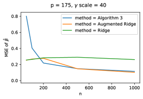
The average MSE is computed for ridge regression and augmented ridge regression just as for substitute adjustment. Figure 4 shows results for $p=125$ and $p=175$ . These two values of $p$ correspond to asymptotic (as $p$ stays fixed and $n\to\infty$ ) mislabeling rates $\delta$ around $7\%$ and $2\%$ , respectively.

We see that both alternative estimators outperform Algorithm 3 when the sample size is too small to learn $Z$ reliably. However, naive linear regression is biased, and so is ridge regression (even asymptotically), and its performance does not improve as the sample size, $n$ , increases. Substitute adjustment as well as augmented ridge regression adjust for $\hat{Z}$ , and their performance improve with $n$ , despite the fact that $p$ is too small to recover $Z$ exactly. When $n$ and the amount of unobserved confounding is sufficiently large, both of these estimators outperform ridge regression. Note that it is unsurprising that the augmented ridge estimator performs similarly to Algorithm 3 for large sample sizes, because after adjusting for the substitutes, the $x_{i,k}$ -residuals are roughly orthogonal if the substitutes give accurate recovery, and a joint regression will give estimates similar to those of the marginal regressions.

We made a couple of observations (data not shown) during the simulation study. We experimented with changing the mixture distributions to other sub-Gaussian distributions as well as to the Laplace distribution and got similar results as shown here using the Gaussian distribution. We also implemented sample splitting, and though Proposition 4 assumes sample splitting, we found that the improved estimation accuracy attained by using all available data for the tensor decomposition outweighs the benefit of sample splitting in the recovery stage.

In conclusion, our simulations show that for reasonable finite $n$ and $p$ , it is possible to recover the latent variables sufficiently well for substitute adjustment to be a better alternative than naive linear or ridge regression in settings where the unobserved confounding is sufficiently large.

5. Discussion

We break the discussion into three parts. In the first part we revisit the discussion about the causal interpretation of the target parameters $\chi_{x}^{i}$ treated in this paper. In the second part we discuss substitute adjustment as a method for estimation of these parameters as well as the assumption-lean parameters $\beta_{i}$ . In the third part we discuss possible extensions of our results

5.1. Causal interpretations

The main causal question is whether a contrast of the form $\chi_{x}^{i}-\chi_{x_{0}}^{i}$ has a causal interpretation as an average treatment effect. The framework in (Wang & Blei, 2019) and the subsequent criticisms by D’Amour (2019) and Ogburn et al. (2020) are based on the $X_{i}$ -s all being causes of $Y$ , and on the possibility of unobserved confounding. Notably, the latent variable $Z$ to be recovered is not equal to an unobserved confounder, but Wang & Blei (2019) argue that using the deconfounder allows us to weaken the assumption of “no unmeasured confounding” to “no unmeasured single-cause confounding”. The assumptions made in (Wang & Blei, 2019) did not fully justify this claim, and we found it difficult to understand precisely what the causal assumptions related to $Z$ were.

Mathematically precise assumptions that allow for identification of causal parameters from a finite number of causes, $X_{1},\ldots,X_{p}$ , via deconfounding are stated as Assumptions 1 and 2 in (Wang & Blei, 2020). We find these assumptions regarding recovery of $Z$ (also termed “pinpointing” in the context of the deconfounder) for finite $p$ implausible. Moreover, the entire framework of the deconfounder rests on the causal assumption of “weak unconfoundedness” in Assumption 1 and Theorem 1 of (Wang & Blei, 2020), which might be needed for a causal interpretation but is unnecessary for the deconfounder algorithm to estimate a meaningful target parameter.

We find it beneficial to disentangle the causal interpretation from the definition of the target parameter. By defining the target parameter entirely in terms of the observational distribution of observed (or, at least, observable) variables, we can discuss the properties of the statistical method of substitute adjustment without making causal claims. We have shown that substitute adjustment under our Assumption 2 on the latent variable model targets the adjusted mean irrespectively of any unobserved confounding. Grimmer et al. (2023) present a similar view. The contrast $\chi_{x}^{i}-\chi_{x_{0}}^{i}$ might have a causal interpretation in specific applications, but substitute adjustment as a statistical method does not rely on such an interpretation or assumptions needed to justify such an interpretation. In any specific application with multiple causes and potential unobserved confounding, substitute adjustment might be a useful method for deconfounding, but depending on the context and the causal assumptions we are willing to make, other methods could be preferable (Miao et al., 2023).

5.2. Substitute adjustment: interpretation, merits and deficits

We define the target parameter as an adjusted mean when adjusting for an infinite number of variables. Clearly, this is a mathematical idealization of adjusting for a large number of variables, but it also has some important technical consequences. First, the recovery Assumption 2(2) is a more plausible modelling assumption than recovery from a finite number of variables. Second, it gives a clear qualitative difference between the adjusted mean of one (or any finite number of) variables and regression on all variables. Third, the natural requirement in Assumption 2(2) that $Z$ can be recovered from $\mathbf{X}_{-i}$ for any $i$ replaces the minimality of a “multi-cause separator” from (Wang & Blei, 2020). Our assumption is that $\sigma(Z)$ is sufficiently minimal in a very explicit way, which ensures that $Z$ does not contain information unique to any single $X_{i}$ .

Grimmer et al. (2023) come to a similar conclusion as we do: that the target parameter of substitute adjustment (and the deconfounder) is the adjusted mean $\chi^{i}_{x}$ , where you adjust for an infinite number of variables. They argue forcefully that substitute adjustment, using a finite number $p$ of variables, does not have an advantage over naive regression, that is, over estimating the regression function $\mathbb{E}\left[Y\mid X_{1}=x_{1},\ldots,X_{p}=x_{p}\right]$ directly. With $i=1$ , say, they argue that substitute adjustment is effectively assuming a partially linear, semiparametric regression model

\mathbb{E}\left[Y\mid X_{1}=x_{1},\ldots,X_{p}=x_{p}\right]=\beta_{0}+\beta_{1}x_{1}+h(x_{2},\ldots,x_{p}),

with the specific constraint that $h(x_{2},\ldots,x_{p})=g(\hat{z})=g(f^{(p)}(x_{2},\ldots,x_{p}))$ . We agree with their analysis and conclusion; substitute adjustment is implicitly a way of making assumptions about $h$ . It is also a way to leverage those assumptions, either by shrinking the bias compared to directly estimating a misspecified (linear, say) $h$ , or by improving efficiency over methods that use a too flexible model of $h$ . We believe there is room for further studies of such bias and efficiency tradeoffs.

We also believe that there are two potential benefits of substitute adjustment, which are not brought forward by Grimmer et al. (2023). First, the latent variable model can be estimated without access to outcome observations. This means that the inner part of $h=g\circ f^{(p)}$ could, potentially, be estimated very accurately on the basis of a large sample $\mathcal{S}_{0}$ in cases where it would be difficult to estimate the composed map $h$ accurately from $\mathcal{S}$ alone. Second, when $p$ is very large, e.g., in the millions, but $Z$ is low-dimensional, there can be huge computational advantages to running $p$ small parallel regressions compared to just one naive linear regression of $Y$ on all of $\mathbf{X}_{1:p}$ , let alone $p$ naive partially linear regressions.

5.3. Possible extensions

We believe that our error bound in Theorem 1 is an interesting result, which in a precise way bounds the error of an OLS estimator in terms of errors in the regressors. This result is closely related to the classical literature on errors-in-variables models (or measurement error models) (Durbin, 1954; Cochran, 1968; Schennach, 2016), though this literature focuses on methods for bias correction when the errors are non-vanishing. We see two possible extensions of our result. For one, Theorem 1 could easily be generalized to $E=\mathbb{R}^{d}$ . In addition, it might be possible to apply the bias correction techniques developed for errors-in-variables to improve the finite sample properties of the substitute adjustment estimator.

Our analysis of the recovery error could also be extended. The concentration inequalities in Section 3.3 are unsurprising, but developed to match our specific needs for a high-dimensional analysis with as few assumptions as possible. For more refined results on finite mixture estimation see, e.g., (Heinrich & Kahn, 2018), and see (Ndaoud, 2022) for optimal recovery when $K=2$ and the mixture distributions are Gaussian. In cases where the mixture distributions are Gaussian, it is also plausible that specialized algorithms such as (Kalai et al., 2012; Gandhi & Borns-Weil, 2016) are more efficient than the methods we consider based on conditional means only.

One general concern with substitute adjustment is model misspecification. We have done our analysis with minimal distributional assumptions, but there are, of course, two fundamental assumptions: the assumption of conditional independence of the $X_{i}$ -s given the latent variable $Z$ , and the assumption that $Z$ takes values in a finite set of size $K$ . An important extension of our results is to study robustness to violations of these two fundamental assumptions. We have also not considered estimation of $K$ , and it would likewise be relevant to understand how that affects the substitute adjustment estimator.

Acknowledgments

We thank Alexander Mangulad Christgau for helpful input. JA and NRH were supported by a research grant (NNF20OC0062897) from Novo Nordisk Fonden. JA also received funding from the European Union’s Horizon 2020 research and innovation programme under Marie Skłodowska-Curie grant agreement No 801199.

Appendix A Proofs and auxiliary results

A.1. Proofs of results in Section 2.1

Proof of Proposition 1.

Since $X_{i}$ as well as $\mathbf{X}_{-i}$ take values in Borel spaces, there exists a regular conditional distribution given $Z=z$ of each (Kallenberg, 2021, Theorem 8.5). These are denoted $P^{i}_{z}$ and $P^{-i}_{z}$ , respectively. Moreover, Assumption 2(2) and the Doob-Dynkin lemma (Kallenberg, 2021, Lemma 1.14) imply that for each $i\in\mathbb{N}$ there is a measurable map $f_{i}:\mathbb{R}^{\mathbb{N}}\to E$ such that $Z=f_{i}(\mathbf{X}_{-i})$ . This implies that $P^{-i}(B)=\int P^{-i}_{z}(B)P^{Z}(\mathrm{d}z)$ for $B\subseteq\mathbb{R}^{\mathbb{N}}$ measurable.

Since $Z=f_{i}(\mathbf{X}_{-i})$ it holds that $f_{i}(P^{-i})=P^{Z}$ , and furthermore that $P^{-i}_{z}(f^{-1}_{i}(\{z\}))=1$ . Assumption 2(1) implies that $X_{i}$ and $\mathbf{X}_{-i}$ are conditionally independent given $Z$ , thus for $A,C\subseteq\mathbb{R}$ and $B\subseteq E$ measurable sets and $\tilde{B}=f_{i}^{-1}(B)\subseteq\mathbb{R}^{\mathbb{N}}$ ,

	$\displaystyle\mathbb{P}(X_{i}\in A,Z\in B,Y\in C)$	$\displaystyle=\mathbb{P}(X_{i}\in A,\mathbf{X}_{-i}\in\tilde{B},Y\in C)$
		$\displaystyle=\int 1_{A}(x)1_{\tilde{B}}(\mathbf{x})P_{x,\mathbf{x}}^{i}(C)P(\mathrm{d}x,\mathrm{d}\mathbf{x})$
		$\displaystyle=\int 1_{A}(x)1_{\tilde{B}}(\mathbf{x})\,P_{x,\mathbf{x}}^{i}(C)\int P_{z}^{i}\otimes P_{z}^{-i}(\mathrm{d}x,\mathrm{d}\mathbf{x})P^{Z}(\mathrm{d}z)$
		$\displaystyle=\iiint 1_{A}(x)1_{\tilde{B}}(\mathbf{x})\,P_{x,\mathbf{x}}^{i}(C)P_{z}^{i}(\mathrm{d}x)P_{z}^{-i}(\mathrm{d}\mathbf{x})P^{Z}(\mathrm{d}z)$
		$\displaystyle=\iiint 1_{A}(x)1_{B}(z)\,\int P_{x,\mathbf{x}}^{i}(C)P_{z}^{-i}(\mathrm{d}\mathbf{x})P_{z}^{i}(\mathrm{d}x)P^{Z}(\mathrm{d}z)$
		$\displaystyle=\iint 1_{A}(x)1_{B}(z)\,Q^{i}_{x,z}(C)P_{z}^{i}(\mathrm{d}x)P^{Z}(\mathrm{d}z).$

Hence $Q^{i}_{x,z}$ is a regular conditional distribution of $Y$ given $(X_{i},Z)=(x,z)$ .

We finally find that

	$\displaystyle\chi_{x}^{i}$	$\displaystyle=\iint y\,P^{i}_{x,\mathbf{x}}(\mathrm{d}y)P^{-i}(\mathrm{d}\mathbf{x})$
		$\displaystyle=\iiint y\,P^{i}_{x,\mathbf{x}}(\mathrm{d}y)P^{-i}_{z}(\mathrm{d}\mathbf{x})P^{Z}(\mathrm{d}z)$
		$\displaystyle=\iint y\,\int P^{i}_{x,\mathbf{x}}(\mathrm{d}y)P^{-i}_{z}(\mathrm{d}\mathbf{x})P^{Z}(\mathrm{d}z)$
		$\displaystyle=\iint y\,Q^{i}_{z,\mathbf{x}}(\mathrm{d}y)P^{Z}(\mathrm{d}z).$

∎

Proof of Proposition 2.

We find that

	$\displaystyle\operatorname{Cov}\left[X_{i},Y\mid Z\right]$	$\displaystyle=\mathbb{E}\left[(X_{i}-\mathbb{E}[X_{i}\mid Z])Y\mid Z\right]$
		$\displaystyle=\mathbb{E}\left[\mathbb{E}\left[(X_{i}-\mathbb{E}[X_{i}\mid Z])Y\mid X_{i},Z\right]\mid Z\right]$
		$\displaystyle=\mathbb{E}\left[(X_{i}-\mathbb{E}[X_{i}\mid Z])\mathbb{E}\left[Y\mid X_{i},Z\right]\mid Z\right]$
		$\displaystyle=\mathbb{E}\left[(X_{i}-\mathbb{E}[X_{i}\mid Z])b_{X_{i}}^{i}(Z)\mid Z\right]$
		$\displaystyle=\operatorname{Cov}\left[X_{i},b^{i}_{X_{i}}(Z)\mid Z\right],$

which shows (9). From this representation, if $b_{x}^{i}(z)=b^{i}(z)$ does not depend on $x$ , $b^{i}(Z)$ is $\sigma(Z)$ -measurable and $\operatorname{Cov}\left[X_{i},b^{i}(Z)\mid Z\right]=0$ , whence $\beta_{i}=0$ .

If $b^{i}_{x}(z)=\beta_{i}^{\prime}(z)x+\eta_{-i}(z)$ ,

\operatorname{Cov}\left[X_{i},b^{i}_{X_{i}}(Z)\mid Z\right]=\operatorname{Cov}\left[X_{i},\beta_{i}^{\prime}(Z)X_{i}+\eta_{-i}(Z)\mid Z\right]=\beta_{i}^{\prime}(Z)\operatorname{Var}\left[X_{i}\mid Z\right],

and (10) follows. ∎

A.2. Auxiliary results related to Section 3.2 and proof of Theorem 1

Let $\mathbf{Z}$ denote the $n\times K$ matrix of dummy variable encodings of the $z_{k}$ -s, and let $\hat{\mathbf{Z}}$ denote the similar matrix for the substitutes $\hat{z}_{k}$ -s. With $P_{\mathbf{Z}}$ and $P_{\hat{\mathbf{Z}}}$ the orthogonal projections onto the column spaces of $\mathbf{Z}$ and $\hat{\mathbf{Z}}$ , respectively, we can write the estimator from Algorithm 3 as

(27)

\widehat{\beta}^{\mathrm{sub}}_{i}=\frac{\langle\mathbf{x}_{i}-P_{\hat{\mathbf{Z}}}\mathbf{x}_{i},\mathbf{y}-P_{\hat{\mathbf{Z}}}\mathbf{y}\rangle}{\|\mathbf{x}_{i}-P_{\hat{\mathbf{Z}}}\mathbf{x}_{i}\|_{2}^{2}}.

Here $\mathbf{x}_{i},\mathbf{y}\in\mathbb{R}^{n}$ denote the $n$ -vectors of $x_{i,k}$ -s and $y_{k}$ -s, respectively, and $\langle\cdot,\cdot\rangle$ is the standard inner product on $\mathbb{R}^{n}$ , so that, e.g., $\|\mathbf{y}\|_{2}^{2}=\langle\mathbf{y},\mathbf{y}\rangle$ . The estimator, had we observed the latent variables, is similarly given as

(28)

\hat{\beta}_{i}=\frac{\langle\mathbf{x}_{i}-P_{\mathbf{Z}}\mathbf{x}_{i},\mathbf{y}-P_{\mathbf{Z}}\mathbf{y}\rangle}{\|\mathbf{x}_{i}-P_{\mathbf{Z}}\mathbf{x}_{i}\|_{2}^{2}}.

The proof of Theorem 1 is based on the following bound on the difference between the projection matrices.

Lemma 1.

Let $\alpha$ and $\delta$ be as defined by (16) and (17). If $\alpha>0$ it holds that

(29)

\|P_{\mathbf{Z}}-P_{\hat{\mathbf{Z}}}\|_{2}\leq\sqrt{\frac{2\delta}{\alpha}},

where $\|\cdot\|_{2}$ above denotes the operator $2$ -norm also known as the spectral norm.

Proof.

When $\alpha>0$ , the matrices $\mathbf{Z}$ and $\hat{\mathbf{Z}}$ have full rank $K$ . Let $\mathbf{Z}^{+}=(\mathbf{Z}^{T}\mathbf{Z})^{-1}\mathbf{Z}^{T}$ and $\hat{\mathbf{Z}}^{+}=(\hat{\mathbf{Z}}^{T}\hat{\mathbf{Z}})^{-1}\hat{\mathbf{Z}}^{T}$ denote the Moore-Penrose inverses of $\mathbf{Z}$ and $\hat{\mathbf{Z}}$ , respectively. Then $P_{\mathbf{Z}}=\mathbf{Z}\mathbf{Z}^{+}$ and $P_{\hat{\mathbf{Z}}}=\hat{\mathbf{Z}}\hat{\mathbf{Z}}^{+}$ . By Theorems 2.3 and 2.4 in (Stewart, 1977),

\|P_{\mathbf{Z}}-P_{\hat{\mathbf{Z}}}\|_{2}\leq\min\left\{\|\mathbf{Z}^{+}\|_{2},\|\hat{\mathbf{Z}}^{+}\|_{2}\right\}\ \|\mathbf{Z}-\hat{\mathbf{Z}}\|_{2}.

The operator $2$ -norm $\|\mathbf{Z}^{+}\|_{2}$ is the square root of the largest eigenvalue of

(\mathbf{Z}^{T}\mathbf{Z})^{-1}=\left(\begin{array}[]{cccc}n(1)^{-1}&0&\ldots&0\\ 0&n(2)^{-1}&\ldots&0\\ \vdots&\vdots&\ddots&\vdots\\ 0&0&\ldots&n(K)^{-1}\end{array}\right).

Whence $\|\mathbf{Z}^{+}\|_{2}\leq(n_{\min})^{-1/2}=(\alpha n)^{-1/2}$ . The same bound is obtained for $\|\hat{\mathbf{Z}}^{+}\|_{2}$ , which gives

\|P_{\mathbf{Z}}-P_{\hat{\mathbf{Z}}}\|_{2}\leq\frac{1}{\sqrt{\alpha n}}\ \|\mathbf{Z}-\hat{\mathbf{Z}}\|_{2}.

We also have that

\|\mathbf{Z}-\hat{\mathbf{Z}}\|_{2}^{2}\leq\|\mathbf{Z}-\hat{\mathbf{Z}}\|_{F}^{2}=\sum_{k=1}^{n}\sum_{i=1}^{p}(\mathbf{Z}_{k,i}-\hat{\mathbf{Z}}_{k,i})^{2}=2\delta n,

because $\sum_{i=1}^{p}(\mathbf{Z}_{k,i}-\hat{\mathbf{Z}}_{k,i})^{2}=2$ precisely for those $k$ with $\hat{z}_{k}\neq z_{k}$ and $0$ otherwise. Combining the inequalities gives (29). ∎

Before proceeding with the proof of Theorem 1, note that

\sum_{k=1}^{n}(x_{i,k}-\overline{\mu}_{i}(z_{k}))^{2}=\|\mathbf{x}_{i}-P_{\mathbf{Z}}\mathbf{x}_{i}\|_{2}^{2}=\|(I-P_{\mathbf{Z}})\mathbf{x}_{i}\|_{2}^{2}\leq\|\mathbf{x}_{i}\|_{2}^{2}

since $(I-P_{\mathbf{Z}})$ is a projection. Similarly, $\sum_{k=1}^{n}(x_{i,k}-\hat{\mu}_{i}(\hat{z}_{k}))^{2}=\|\mathbf{x}_{i}-P_{\hat{\mathbf{Z}}}\mathbf{x}_{i}\|_{2}^{2}\leq\|\mathbf{x}\|_{2}^{2}$ , thus

\rho=\frac{\min\left\{\|\mathbf{x}_{i}-P_{\mathbf{Z}}\mathbf{x}_{i}\|_{2}^{2},\|\mathbf{x}_{i}-P_{\hat{\mathbf{Z}}}\mathbf{x}_{i}\|_{2}^{2}\right\}}{\|\mathbf{x}_{i}\|_{2}^{2}}\leq 1.

Proof of Theorem 1.

First note that since $I-P_{\hat{\mathbf{Z}}}$ is an orthogonal projection,

\langle\mathbf{x}_{i}-P_{\hat{\mathbf{Z}}}\mathbf{x}_{i},\mathbf{y}-P_{\hat{\mathbf{Z}}}\mathbf{y}\rangle=\langle\mathbf{x}_{i},(I-P_{\hat{\mathbf{Z}}})\mathbf{y}\rangle

and similarly for the other inner product in (28). Moreover,

\langle\mathbf{x}_{i},(I-P_{\hat{\mathbf{Z}}})\mathbf{y}\rangle-\langle\mathbf{x}_{i},(I-P_{\mathbf{Z}})\mathbf{y}\rangle=\langle\mathbf{x}_{i},(P_{\mathbf{Z}}-P_{\hat{\mathbf{Z}}})\mathbf{y}\rangle

and

\|(I-P_{\mathbf{Z}})\mathbf{x}_{i}\|_{2}^{2}-\|(I-P_{\hat{\mathbf{Z}}})\mathbf{x}_{i}\|_{2}^{2}=\|(P_{\hat{\mathbf{Z}}}-P_{\mathbf{Z}})\mathbf{x}_{i}\|_{2}^{2}.

We find that

	$\displaystyle\widehat{\beta}^{\mathrm{sub}}_{i}-\hat{\beta}_{i}$	$\displaystyle=\frac{\langle\mathbf{x}_{i},(I-P_{\hat{\mathbf{Z}}})\mathbf{y}\rangle}{\\|(I-P_{\hat{\mathbf{Z}}})\mathbf{x}_{i}\\|_{2}^{2}}-\frac{\langle\mathbf{x}_{i},(I-P_{\mathbf{Z}})\mathbf{y}\rangle}{\\|(I-P_{\mathbf{Z}})\mathbf{x}_{i}\\|_{2}^{2}}$
		$\displaystyle=\langle\mathbf{x}_{i},(I-P_{\hat{\mathbf{Z}}})\mathbf{y}\rangle\left(\frac{1}{\\|(I-P_{\hat{\mathbf{Z}}})\mathbf{x}_{i}\\|_{2}^{2}}-\frac{1}{\\|(I-P_{\mathbf{Z}})\mathbf{x}_{i}\\|_{2}^{2}}\right)$
		$\displaystyle\qquad\qquad+\frac{\langle\mathbf{x}_{i},(I-P_{\hat{\mathbf{Z}}})\mathbf{y}\rangle-\langle\mathbf{x}_{i},(I-P_{\mathbf{Z}})\mathbf{y}\rangle}{\\|(I-P_{\mathbf{Z}})\mathbf{x}_{i}\\|_{2}^{2}}$
		$\displaystyle=\langle\mathbf{x}_{i},(I-P_{\hat{\mathbf{Z}}})\mathbf{y}\rangle\left(\frac{\\|(P_{\hat{\mathbf{Z}}}-P_{\mathbf{Z}})\mathbf{x}_{i}\\|_{2}^{2}}{\\|(I-P_{\hat{\mathbf{Z}}})\mathbf{x}_{i}\\|_{2}^{2}\\|(I-P_{\mathbf{Z}})\mathbf{x}_{i}\\|_{2}^{2}}\right)$
		$\displaystyle\qquad\qquad+\frac{\langle\mathbf{x}_{i},(P_{\mathbf{Z}}-P_{\hat{\mathbf{Z}}})\mathbf{y}\rangle}{\\|(I-P_{\mathbf{Z}})\mathbf{x}_{i}\\|_{2}^{2}}.$

This gives the following inequality, using that $\rho\leq 1$ ,

	$\displaystyle\|\widehat{\beta}^{\mathrm{sub}}_{i}-\hat{\beta}_{i}\|$	$\displaystyle\leq\frac{\\|P_{\mathbf{Z}}-P_{\hat{\mathbf{Z}}}\\|_{2}\\|\mathbf{x}_{i}\\|_{2}^{3}\\|\mathbf{y}\\|_{2}}{\rho^{2}\\|\mathbf{x}_{i}\\|^{4}_{2}}+\frac{\\|P_{\mathbf{Z}}-P_{\hat{\mathbf{Z}}}\\|_{2}\\|\mathbf{x}_{i}\\|_{2}\\|\mathbf{y}\\|_{2}}{\rho\\|\mathbf{x}_{i}\\|^{2}_{2}}$
		$\displaystyle=\left(\frac{1}{\rho^{2}}+\frac{1}{\rho}\right)\\|P_{\mathbf{Z}}-P_{\hat{\mathbf{Z}}}\\|_{2}\frac{\\|\mathbf{y}\\|_{2}}{\\|\mathbf{x}_{i}\\|_{2}}$
		$\displaystyle\leq\frac{2}{\rho^{2}}\\|P_{\mathbf{Z}}-P_{\hat{\mathbf{Z}}}\\|_{2}\frac{\\|\mathbf{y}\\|_{2}}{\\|\mathbf{x}_{i}\\|_{2}}.$

Combining this inequality with (29) gives (19). ∎

A.3. Auxiliary concentration inequalities. Proofs of Propositions 3 and 4

Lemma 2.

Suppose that Assumption 4 holds. Let $\check{\boldsymbol{\mu}}_{1:p}(z)\in\mathbb{R}^{p}$ for $z\in E$ and let $\hat{Z}=\operatorname*{arg\,min}_{z}\|\mathbf{X}_{1:p}-\check{\boldsymbol{\mu}}_{1:p}(z)\|_{2}$ . Suppose that $R_{z,v}^{(p)}\leq\frac{1}{10}$ for all $z,v\in E$ with $v\neq z$ then

(30)

\mathbb{P}(\hat{Z}=v\mid Z=z)\leq\frac{25\sigma_{\max}^{2}}{\|\boldsymbol{\mu}_{1:p}(z)-\boldsymbol{\mu}_{1:p}(v)\|_{2}^{2}}.

Proof.

Since $p$ is fixed throughout the proof, we simplify the notation by dropping the $1\!\!:\!\!p$ subscript and use, e.g., $\mathbf{X}$ and $\boldsymbol{\mu}$ to denote the $\mathbb{R}^{p}$ -vectors $\mathbf{X}_{1:p}$ and $\boldsymbol{\mu}_{1:p}$ , respectively.

Fix also $z,v\in E$ with $v\neq z$ and observe first that

	$\displaystyle(\hat{Z}=v)$	$\displaystyle\subseteq\left(\norm{\mathbf{X}-\check{\boldsymbol{\mu}}(v)}_{2}<\norm{\mathbf{X}-\check{\boldsymbol{\mu}}(z)}_{2}\right)$
		$\displaystyle=\left(\langle\mathbf{X}-\check{\boldsymbol{\mu}}(z),\check{\boldsymbol{\mu}}(z)-\check{\boldsymbol{\mu}}(v)\rangle<-\tfrac{1}{2}\norm{\check{\boldsymbol{\mu}}(z)-\check{\boldsymbol{\mu}}(v)}^{2}_{2}\right)$
		$\displaystyle=\Big{(}\langle\mathbf{X}-\boldsymbol{\mu}(z),\check{\boldsymbol{\mu}}(z)-\check{\boldsymbol{\mu}}(v)\rangle<$
		$\displaystyle\qquad\qquad-\left(\tfrac{1}{2}\norm{\check{\boldsymbol{\mu}}(z)-\check{\boldsymbol{\mu}}(v)}^{2}_{2}+\langle\boldsymbol{\mu}(z)-\check{\boldsymbol{\mu}}(z),\check{\boldsymbol{\mu}}(z)-\check{\boldsymbol{\mu}}(v)\rangle\right)\Big{)}.$

The objective is to bound the probability of the event above using Chebyshev’s inequality. To this end, we first use the Cauchy-Schwarz inequality to get

	$\displaystyle\tfrac{1}{2}\norm{\check{\boldsymbol{\mu}}(z)-\check{\boldsymbol{\mu}}(v)}^{2}_{2}$	$\displaystyle+\langle\boldsymbol{\mu}(z)-\check{\boldsymbol{\mu}}(z),\check{\boldsymbol{\mu}}(z)-\check{\boldsymbol{\mu}}(v)\rangle$
		$\displaystyle\geq\tfrac{1}{2}\norm{\check{\boldsymbol{\mu}}(z)-\check{\boldsymbol{\mu}}(v)}^{2}_{2}-\\|\boldsymbol{\mu}(z)-\check{\boldsymbol{\mu}}(z)\\|_{2}\\|\check{\boldsymbol{\mu}}(z)-\check{\boldsymbol{\mu}}(v)\\|_{2}$
		$\displaystyle=\norm{\boldsymbol{\mu}(z)-\boldsymbol{\mu}(v)}_{2}^{2}\left(\tfrac{1}{2}B_{z,v}^{2}-R_{z,v}^{(p)}B_{z,v}\right),$

where

B_{z,v}=\frac{\norm{\check{\boldsymbol{\mu}}(z)-\check{\boldsymbol{\mu}}(v)}_{2}}{\norm{\boldsymbol{\mu}(z)-\boldsymbol{\mu}(v)}_{2}}.

The triangle and reverse triangle inequality give that

	$\displaystyle\norm{\check{\boldsymbol{\mu}}(z)-\check{\boldsymbol{\mu}}(v)}_{2}$	$\displaystyle\leq\norm{\boldsymbol{\mu}(z)-\boldsymbol{\mu}(v)}_{2}+\norm{\check{\boldsymbol{\mu}}(z)-\boldsymbol{\mu}(z)}_{2}+\norm{\boldsymbol{\mu}(v)-\check{\boldsymbol{\mu}}(v)}_{2}$
	$\displaystyle\norm{\check{\boldsymbol{\mu}}(z)-\check{\boldsymbol{\mu}}(v)}_{2}$	$\displaystyle\geq\Big{\|}\norm{\boldsymbol{\mu}(z)-\boldsymbol{\mu}(v)}_{2}-\norm{\boldsymbol{\mu}(z)-\check{\boldsymbol{\mu}}(z)}_{2}-\norm{\boldsymbol{\mu}(v)-\check{\boldsymbol{\mu}}(v)}_{2}\Big{\|},$

and dividing by $\norm{\boldsymbol{\mu}(z)-\boldsymbol{\mu}(v)}_{2}$ combined with the bound $\tfrac{1}{10}$ on the relative errors yield

	$\displaystyle B_{z,v}$	$\displaystyle\leq 1+R_{z,v}^{(p)}+R_{v,z}^{(p)}\leq\frac{6}{5},$
	$\displaystyle B_{z,v}$	$\displaystyle\geq\Big{\|}1-R_{z,v}^{(p)}-R_{v,z}^{(p)}\Big{\|}\geq\frac{4}{5}.$

This gives

\tfrac{1}{2}B_{z,v}^{2}-R_{z,v}^{(p)}B_{z,v}\geq\tfrac{1}{2}B_{z,v}^{2}-\tfrac{1}{10}B_{z,v}\geq\tfrac{6}{25}

since the function $b\mapsto b^{2}-\tfrac{2}{10}b$ is increasing for $b\geq\tfrac{4}{5}$ .

Introducing the variables $W_{i}=(X_{i}-\mu_{i}(z))(\check{\mu}_{i}(z)-\check{\mu}_{i}(v))$ we conclude that

(31)

\displaystyle(\hat{Z}=v)

\displaystyle\subseteq\left(\sum_{i=1}^{p}W_{i}<-\tfrac{6}{25}\norm{\boldsymbol{\mu}(z)-\boldsymbol{\mu}(v)}_{2}^{2}\right).

Note that $\mathbb{E}[W_{i}\mid Z=z]=0$ and $\operatorname{Var}[W_{i}\mid Z=z]=(\check{\mu}_{i}(z)-\check{\mu}_{i}(v))^{2}\sigma^{2}_{i}(z)$ , and by Assumption 4, the $W_{i}$ -s are conditionally independent given $Z=z$ , so Chebyshev’s inequality gives that

	$\displaystyle\mathbb{P}(\hat{Z}=v\mid Z=z)$	$\displaystyle\leq\mathbb{P}\left(\sum_{i=1}^{p}W_{i}<-\tfrac{6}{25}\norm{\boldsymbol{\mu}(z)-\boldsymbol{\mu}(v)}_{2}^{2}\;\middle\|\;Z=z\right)$
		$\displaystyle\leq\left(\frac{25}{6}\right)^{2}\frac{\sum_{i=1}^{p}(\check{\mu}_{i}(z)-\check{\mu}_{i}(v))^{2}\sigma^{2}_{i}(z)}{\norm{\boldsymbol{\mu}(z)-\boldsymbol{\mu}(v)}_{2}^{4}}$
		$\displaystyle\leq\left(\frac{25}{6}\right)^{2}\frac{\sigma^{2}_{\max}\norm{\check{\boldsymbol{\mu}}(z)-\check{\boldsymbol{\mu}}(v)}_{2}^{2}}{\norm{\boldsymbol{\mu}(z)-\boldsymbol{\mu}(v)}_{4}^{2}}$
		$\displaystyle\leq\left(\frac{25}{6}\right)^{2}B_{z,v}^{2}\frac{\sigma^{2}_{\max}}{\norm{\boldsymbol{\mu}(z)-\boldsymbol{\mu}(v)}_{2}^{2}}$
		$\displaystyle\leq\frac{25\sigma^{2}_{\max}}{\norm{\boldsymbol{\mu}(z)-\boldsymbol{\mu}(v)}_{2}^{2}},$

where we, for the last inequality, used that $B_{z,v}^{2}\leq\left(\frac{6}{5}\right)^{2}$ . ∎

Before proceeding to the concentration inequality for sub-Gaussian distributions, we use Lemma 2 to prove Proposition 3.

Proof of Proposition 3.

Suppose that $i=1$ for convenience. We take $\check{\boldsymbol{\mu}}_{1:p}(z)=\boldsymbol{\mu}_{1:p}(z)$ for all $p\in\mathbb{N}$ and $z\in E$ and write $\hat{Z}_{p}=\operatorname*{arg\,min}_{z}\|\mathbf{X}_{2:p}-\boldsymbol{\mu}_{2:p}(z)\|_{2}$ for the prediction of $Z$ based on the coordinates $2,\ldots,p$ . With this oracle choice of $\check{\boldsymbol{\mu}}_{1:p}(z)$ , the relative errors are zero, thus the bound (30) holds, and Lemma 2 gives

	$\displaystyle\mathbb{P}\left(\hat{Z}_{p}\neq Z\right)$	$\displaystyle=\sum_{z}\sum_{v\neq z}\mathbb{P}\left(\hat{Z}_{p}=v,Z=z\right)$
		$\displaystyle=\sum_{z}\sum_{v\neq z}\mathbb{P}\left(\hat{Z}_{p}=v\;\middle\|\;Z=z\right)\mathbb{P}\left(Z=z\right)$
		$\displaystyle\leq\frac{C}{\min_{z\neq v}\norm{\boldsymbol{\mu}_{2:p}(z)-\boldsymbol{\mu}_{2:p}(v)}_{2}^{2}}$

with $C$ a constant independent of $p$ . By (14), $\min_{z\neq v}\norm{\boldsymbol{\mu}_{2:p}(z)-\boldsymbol{\mu}_{2:p}(v)}_{2}^{2}\to\infty$ for $p\to\infty$ , and by choosing a subsequence, $p_{r}$ , we can ensure that $\mathbb{P}\left(\hat{Z}_{p_{r}}\neq Z\right)\leq\frac{1}{r^{2}}.$ Then $\sum_{r=1}^{\infty}\mathbb{P}\left(\hat{Z}_{p_{r}}\neq Z\right)<\infty$ , and by Borel-Cantelli’s lemma,

\mathbb{P}\left(\hat{Z}_{p_{r}}\neq Z\ \text{infinitely often}\right)=0.

That is, $\mathbb{P}\left(\hat{Z}_{p_{r}}=Z\ \text{eventually}\right)=1$ , which shows that we can recover $Z$ from $(\hat{Z}_{p_{r}})_{r\in\mathbb{N}}$ and thus from $\mathbf{X}_{-1}$ (with probability $1$ ). Defining

Z^{\prime}=\left\{\begin{array}[]{ll}\lim\limits_{r\to\infty}\hat{Z}_{p_{r}}&\qquad\text{if }\hat{Z}_{p_{r}}=Z\text{ eventually}\\ 0&\qquad\text{otherwise}\end{array}\right.

we see that $\sigma(Z^{\prime})\subseteq\sigma(\mathbf{X}_{-1})$ and $Z^{\prime}=Z$ almost surely. Thus if we replace $Z$ by $Z^{\prime}$ in Assumption 4 we see that Assumption 2(2) holds. ∎

Lemma 3.

Consider the same setup as in Lemma 2, that is, Assumption 4 holds and $R_{z,v}^{(p)}\leq\frac{1}{10}$ for all $z,v\in E$ with $v\neq z$ . Suppose, in addition, that the conditional distribution of $X_{i}$ given $Z=z$ is sub-Gaussian with variance factor $v_{\max}$ , independent of $i$ and $z$ , then

(32)

\mathbb{P}(\hat{Z}=v\mid Z=z)\leq\exp\left(-\frac{1}{50v_{\max}}\|\boldsymbol{\mu}_{1:p}(z)-\boldsymbol{\mu}_{1:p}(v)\|_{2}^{2}\right).

Proof.

Recall that $X_{i}$ given $Z=z$ being sub-Gaussian with variance factor $v_{\max}$ means that

\log\mathbb{E}\left[e^{\lambda(X_{i}-\mu_{i}(z))}\;\middle|\;Z=z\right]\leq\frac{1}{2}\lambda^{2}v_{\max}

for $\lambda\in\mathbb{R}$ . Consequently, with $W_{i}$ as in the proof of Lemma 2, and using conditional independence of the $X_{i}$ -s given $Z=z$ ,

	$\displaystyle\log\mathbb{E}\left[e^{\lambda\sum_{i=1}^{p}W_{i}}\;\middle\|\;Z=z\right]$	$\displaystyle=\sum_{i=1}^{p}\log\mathbb{E}\left[e^{\lambda(\check{\mu}_{i}(z)-\check{\mu}_{i}(v))(X_{i}-\mu_{i}(z))}\;\middle\|\;Z=z\right]$
		$\displaystyle\leq\frac{1}{2}\lambda^{2}v_{\max}\sum_{i=1}^{p}(\check{\mu}_{i}(z)-\check{\mu}_{i}(v))^{2}$
		$\displaystyle=\frac{1}{2}\lambda^{2}v_{\max}\\|\check{\boldsymbol{\mu}}_{1:p}(z)-\check{\boldsymbol{\mu}}_{1:p}(v)\\|_{2}^{2}.$

Using (31) in combination with the Chernoff bound gives

	$\displaystyle\mathbb{P}(\hat{Z}=v\mid Z=z)$	$\displaystyle\leq\mathbb{P}\left(\sum_{i=1}^{p}W_{i}<-\tfrac{6}{25}\norm{\boldsymbol{\mu}_{1:p}(z)-\boldsymbol{\mu}_{1:p}(v)}_{2}^{2}\;\middle\|\;Z=z\right)$
		$\displaystyle\leq\exp\left(-\left(\frac{6}{25}\right)^{2}\frac{\norm{\boldsymbol{\mu}_{1:p}(z)-\boldsymbol{\mu}_{1:p}(v)}_{2}^{4}}{2v_{\max}\\|\check{\boldsymbol{\mu}}_{1:p}(z)-\check{\boldsymbol{\mu}}_{1:p}(v)\\|_{2}^{2}}\right)$
		$\displaystyle=\exp\left(-\frac{1}{2v_{\max}}\left(\frac{6}{25}\right)^{2}B_{z,v}^{-2}\norm{\boldsymbol{\mu}_{1:p}(z)-\boldsymbol{\mu}_{1:p}(v)}_{2}^{2}\right)$
		$\displaystyle\leq\exp\left(-\frac{1}{50v_{\max}}\norm{\boldsymbol{\mu}_{1:p}(z)-\boldsymbol{\mu}_{1:p}(v)}_{2}^{2}\right),$

where we, as in the proof of Lemma 2, have used that the bound on the relative error implies that $B_{z,v}\leq\tfrac{6}{5}$ . ∎

Proof of Proposition 4.

The argument proceeds as in the proof of Proposition 3. We first note that

	$\displaystyle\mathbb{P}\left(\hat{Z}\neq Z\right)$	$\displaystyle=\sum_{z}\sum_{v\neq z}\mathbb{P}\left(\hat{Z}=v,Z=z\right)$
		$\displaystyle=\sum_{z}\sum_{v\neq z}\mathbb{P}\left(\hat{Z}=v\;\middle\|\;Z=z\right)\mathbb{P}\left(Z=z\right).$

Lemma 2 then gives

\mathbb{P}\left(\hat{Z}\neq Z\right)\leq\frac{25K\sigma^{2}_{\max}}{\mathrm{sep}(p)}.

If the sub-Gaussian assumption holds, Lemma 3 instead gives

\mathbb{P}\left(\hat{Z}\neq Z\right)\leq K\exp\left(-\frac{\mathrm{sep}(p)}{50v_{\max}}\right).

∎

A.4. Proof of Theorem 2

Proof of Theorem 2.

Recall that

\delta=\frac{1}{n}\sum_{k=1}^{n}1(\hat{z}_{k}\neq z_{k}),

hence by Proposition 4

	$\displaystyle\mathbb{E}[\delta]$	$\displaystyle=\mathbb{P}(\hat{Z}_{k}\neq Z)$
		$\displaystyle\leq\mathbb{P}\left(\hat{Z}_{k}\neq Z\;\middle\|\;\max_{z\neq v}R^{(p)}_{z,v}\leq\tfrac{1}{10}\right)+\mathbb{P}\left(\max_{z\neq v}R^{(p)}_{z,v}>\tfrac{1}{10}\right)$
(33)			$\displaystyle\leq\frac{25K\sigma_{\max}^{2}}{\mathrm{sep}(p)}+K^{2}\max_{z\neq v}\mathbb{P}\left(R^{(p)}_{z,v}>\tfrac{1}{10}\right).$

Both of the terms above tend to $0$ , thus $\delta\overset{P}{\to}0$ .

Now rewrite the bound (19) as

|\widehat{\beta}^{\mathrm{sub}}_{i}-\hat{\beta}_{i}|\leq\sqrt{\delta}\underbrace{\left(\frac{2\sqrt{2}}{\rho^{2}\sqrt{\alpha}}\frac{\|\mathbf{y}\|_{2}}{\|\mathbf{x}_{i}\|_{2}}\right)}_{=L_{n}}

From the argument above, $\sqrt{\delta}\overset{P}{\to}0$ . We will show that the second factor, $L_{n}$ , tends to a constant, $L$ , in probability under the stated assumptions. This will imply that

|\widehat{\beta}^{\mathrm{sub}}_{i}-\hat{\beta}_{i}|\overset{P}{\to}0,

which shows case (1).

Observe first that

\|\mathbf{x}_{i}\|_{2}^{2}=\frac{1}{n}\sum_{k=1}^{n}x_{i,k}^{2}\overset{P}{\to}\mathbb{E}[X_{i}^{2}]\in(0,\infty)

by the Law of Large Numbers, using the i.i.d. assumption and the fact that $\mathbb{E}[X_{i}^{2}]\in(0,\infty)$ by Assumption 4. Similarly, $\|\mathbf{y}\|_{2}^{2}\overset{P}{\to}\mathbb{E}[Y]\in[0,\infty)$ .

Turning to $\alpha$ , we first see that by the Law of Large Numbers,

\frac{n(z)}{n}\overset{P}{\to}\mathbb{P}(Z=z)

for $n\to\infty$ and $z\in E$ . Then observe that for any $z\in E$

|\hat{n}(z)-n(z)|\leq\sum_{k=1}^{n}|1(\hat{z}_{k}=z)-1(z_{k}=z)|\leq\sum_{k=1}^{n}1(\hat{z}_{k}\neq z_{k})\leq n\delta.

Since $\delta\overset{P}{\to}0$ , also

\frac{\hat{n}(z)}{n}\overset{P}{\to}\mathbb{P}(Z=z),

thus

\alpha=\frac{n_{\min}}{n}=\min\left\{\frac{n(1)}{n},\ldots,\frac{n(K)}{n},\frac{\hat{n}(1)}{n},\ldots,\frac{\hat{n}(K)}{n}\right\}\overset{P}{\to}\min_{z\in E}\mathbb{P}(Z=z)\in(0,\infty).

We finally consider $\rho$ , and to this end we first see that

\displaystyle\frac{1}{n}\|(I-P_{\mathbf{Z}})\mathbf{x}_{i}\|_{2}^{2}=\frac{1}{n}\sum_{k=1}^{n}(x_{i,k}-\overline{\mu}(z_{k}))^{2}\overset{P}{\to}\mathbb{E}\left[\sigma_{i}^{2}(Z)\right]\in(0,\infty).

Moreover, using Lemma 1,

	$\displaystyle\left\|\\|(I-P_{\hat{\mathbf{Z}}})\mathbf{x}_{i}\\|_{2}^{2}-\\|(I-P_{\mathbf{Z}})\mathbf{x}_{i}\\|_{2}^{2}\right\|$	$\displaystyle=\left\|\\|(P_{\hat{\mathbf{Z}}}-P_{\mathbf{Z}})\mathbf{x}_{i}\\|_{2}^{2}+2\|\langle(I-P_{\hat{\mathbf{Z}}})\mathbf{x}_{i},(P_{\hat{\mathbf{Z}}}-P_{\mathbf{Z}})\mathbf{x}_{i}\rangle\right\|$
		$\displaystyle\leq\\|P_{\hat{\mathbf{Z}}}-P_{\mathbf{Z}}\\|_{2}^{2}\\|\mathbf{x}_{i}\\|_{2}^{2}+2\\|P_{\hat{\mathbf{Z}}}-P_{\mathbf{Z}}\\|_{2}\\|\mathbf{x}_{i}\\|^{2}_{2}$
		$\displaystyle\leq\left(\frac{2\delta}{\alpha}+\sqrt{\frac{2\delta}{\alpha}}\right)\\|\mathbf{x}_{i}\\|^{2}_{2}.$

Hence

\rho\overset{P}{\to}\frac{\mathbb{E}\left[\sigma_{i}^{2}(Z)\right]}{\mathbb{E}[X_{i}^{2}]}\in(0,\infty).

Combining the limit results,

L_{n}\overset{P}{\to}L=\frac{2\sqrt{2}\mathbb{E}[X_{i}^{2}]^{2}}{\mathbb{E}\left[\sigma_{i}^{2}(Z)\right]^{2}\sqrt{\min_{z\in E}\mathbb{P}(Z=z)}}\sqrt{\frac{\mathbb{E}[Y^{2}]}{\mathbb{E}[X_{i}^{2}]}}\in(0,\infty).

To complete the proof, suppose first that $\frac{\mathrm{sep}(p)}{n}\to\infty$ . Then

\sqrt{n}|\widehat{\beta}^{\mathrm{sub}}_{i}-\hat{\beta}_{i}|\leq\sqrt{n\delta}L_{n}

By (33) we have, under the assumptions given in case (2) of the theorem, that $n\delta\overset{P}{\to}0$ , and case (2) follows.

Finally, in the sub-Gaussian case, and if just $h_{n}=\frac{\mathrm{sep}(p)}{\log(n)}\to\infty$ , then we can replace (33) by the bound

\mathbb{E}[\delta]\leq K\exp\left(-\frac{\mathrm{sep}(p)}{50v_{\max}}\right)+K^{2}\max_{z\neq v}\mathbb{P}\left(R^{(p)}_{z,v}>\tfrac{1}{10}\right).

Multiplying by $n$ , we get that the first term in the bound equals

	$\displaystyle Kn\exp\left(-\frac{\mathrm{sep}(p)}{50v_{\max}}\right)$	$\displaystyle=K\exp\left(-\frac{\mathrm{sep}(p)}{50v_{\max}}+\log(n)\right)$
		$\displaystyle=K\exp\left(\log(n)\left(1-\frac{h_{n}}{50v_{\max}}\right)\right)\to 0$

for $n\to\infty$ . We conclude that the relaxed growth condition on $p$ in terms of $n$ in the sub-Gaussian case is enough to imply $n\delta\overset{P}{\to}0$ , and case (3) follows.

By the decomposition

\sqrt{n}(\widehat{\beta}^{\mathrm{sub}}_{i}-\beta_{i})=\sqrt{n}(\widehat{\beta}^{\mathrm{sub}}_{i}-\widehat{\beta}_{i})+\sqrt{n}(\hat{\beta}_{i}-\beta_{i})

it follows from Slutsky’s theorem that in case (2) as well as case (3),

\sqrt{n}(\widehat{\beta}^{\mathrm{sub}}_{i}-\beta_{i})=\sqrt{n}(\widehat{\beta}_{i}-\beta_{i})+o_{P}(1)\overset{\mathcal{D}}{\to}\mathcal{N}(0,w_{i}^{2}).

∎

Appendix B Gaussian mixture models

This appendix contains an analysis of a latent variable model with a finite $E$ , similar to the one given by Assumption 4, but with Assumption 4(1) strengthened to

X_{i}\mid Z=z\sim\mathcal{N}(\mu_{i}(z),\sigma_{i}^{2}(z)).

Assumptions 4(2), 4(3) and 4(4) are dropped, and the purpose is to understand precisely when Assumption 2(2) holds in this model. That is, when $Z$ can be recovered from $\mathbf{X}_{-i}$ . To keep notation simple, we will show when $Z$ can be recovered from $\mathbf{X}$ , but the analysis and conclusion is the same if we left out a single coordinate.

The key to this analysis is a classical result due to Kakutani. As in Section 2, the conditional distribution of $\mathbf{X}$ given $Z=z$ is denoted $P_{z}$ , and the model assumption is that

(34)

P_{z}=\bigotimes_{i=1}^{\infty}P^{i}_{z}

where $P^{i}_{z}$ is the conditional distribution of $X_{i}$ given $Z=z$ . For Kakutani’s theorem below we do not need the Gaussian assumption; only that $P^{i}_{z}$ and $P^{i}_{v}$ are equivalent (absolutely continuous w.r.t. each other), and we let $\frac{\mathrm{d}P_{z}^{i}}{\mathrm{d}P_{v}^{i}}$ denote the Radon-Nikodym derivative of $P_{z}^{i}$ w.r.t. $P_{v}^{i}$ .

Theorem 3 (Kakutani (1948)).

Let $z,v\in E$ and $v\neq z$ . Then $P_{z}$ and $P_{v}$ are singular if and only if

(35)

\sum_{i=1}^{\infty}-\log\int\sqrt{\frac{\mathrm{d}P_{z}^{i}}{\mathrm{d}P_{v}^{i}}}\ \mathrm{d}P_{v}^{i}=\infty.

Note that

\mathrm{BC}_{z,v}^{i}=\int\sqrt{\frac{\mathrm{d}P_{z}^{i}}{\mathrm{d}P_{v}^{i}}}\ \mathrm{d}P_{v}^{i}

is known as the Bhattacharyya coefficient, while $-\log(\mathrm{BC}_{z,v}^{i})$ and $\sqrt{1-\mathrm{BC}_{z,v}^{i}}$ are known as the Bhattacharyya distance and the Hellinger distance, respectively, between $P^{i}_{z}$ and $P^{i}_{v}$ . Note also that if $P^{i}_{z}=h^{i}_{z}\cdot\lambda$ and $P^{i}_{v}=h^{i}_{v}\cdot\lambda$ for a reference measure $\lambda$ , then

\mathrm{BC}_{z,v}^{i}=\int\sqrt{h_{z}^{i}h_{v}^{i}}\ \mathrm{d}\lambda.

Proposition 5.

Let $P^{i}_{z}$ be the $\mathcal{N}(\mu_{i}(z),\sigma_{i}^{2}(z))$ -distribution for all $i\in\mathbb{N}$ and $z\in E$ . Then $P_{z}$ and $P_{v}$ are singular if and only if either

(36)		$\displaystyle\sum_{i=1}^{\infty}\frac{(\mu_{i}(z)-\mu_{i}(v))^{2}}{\sigma_{i}^{2}(z)+\sigma^{2}_{i}(v)}$	$\displaystyle=\infty\qquad\text{or}$
(37)		$\displaystyle\sum_{i=1}^{\infty}\log\left(\frac{\sigma_{i}^{2}(z)+\sigma^{2}_{i}(v)}{2\sigma_{i}(z)\sigma_{i}(v)}\right)$	$\displaystyle=\infty$

Proof.

Letting $\mu=\mu_{i}(z)$ , $\nu=\mu_{i}(v)$ , $\tau=1/\sigma_{i}(z)$ and $\kappa=1/\sigma_{i}(v)$ we find

	$\displaystyle\mathrm{BC}_{z,v}^{i}$	$\displaystyle=\int\sqrt{\frac{\tau}{\sqrt{2\pi}}\exp(-\frac{\tau^{2}}{2}\quantity(x-\mu)^{2})\frac{\kappa}{\sqrt{2\pi}}\exp(-\frac{\kappa^{2}}{2}\quantity(x-\nu)^{2})}\mathrm{d}x$
		$\displaystyle=\sqrt{\frac{\tau\kappa}{2\pi}}\int\exp(-\frac{(\tau^{2}+\kappa^{2})x^{2}-2(\tau^{2}\mu+\kappa^{2}\nu)x+(\tau^{2}\mu^{2}+\kappa^{2}\nu^{2})}{4})\mathrm{d}x$
		$\displaystyle=\sqrt{\frac{\tau\kappa}{2\pi}}\sqrt{\frac{4\pi}{\tau^{2}+\kappa^{2}}}\exp(\frac{(\tau^{2}\mu+\kappa^{2}\nu)^{2}}{4(\tau^{2}+\kappa^{2})}-\frac{\tau^{2}\mu^{2}+\kappa^{2}\nu^{2}}{4})$
		$\displaystyle=\sqrt{\frac{2\tau\kappa}{\tau^{2}+\kappa^{2}}}\exp(-\frac{\tau^{2}\kappa^{2}(\mu-\nu)^{2}}{4(\tau^{2}+\kappa^{2})})$
		$\displaystyle=\sqrt{\frac{2\sigma_{i}(z)\sigma_{i}(v)}{\sigma^{2}_{i}(z)+\sigma^{2}_{i}(z)}}\exp(-\frac{(\mu_{i}(z)-\mu_{i}(v))^{2}}{4(\sigma^{2}_{i}(z)+\sigma^{2}_{i}(z))}).$

Thus

\sum_{i=1}^{\infty}-\log\left(\mathrm{BC}_{z,v}^{i}\right)=\frac{1}{2}\sum_{i=1}^{\infty}\log\left(\frac{\sigma^{2}_{i}(z)+\sigma_{i}^{2}(v)}{2\sigma_{i}(z)\sigma_{i}(v)}\right)+\frac{1}{4}\sum_{i=1}^{\infty}\frac{(\mu_{i}(z)-\mu_{i}(v))^{2}}{\sigma^{2}_{i}(z)+\sigma_{i}^{2}(v)},

and the result follows from Theorem 3. ∎

Corollary 1.

Let $P^{i}_{z}$ be the $\mathcal{N}(\mu_{i}(z),\sigma_{i}^{2}(z))$ -distribution for all $i\in\mathbb{N}$ and $z\in E$ . There is a mapping $f:\mathbb{R}^{\mathbb{N}}\to E$ such that $Z=f(\mathbf{X})$ almost surely if and only if either (36) or (37) holds.

Proof.

If either (36) or (37) holds, $P_{z}$ and $P_{v}$ are singular whenever $v\neq z$ . This implies that there are measurable subsets $A_{z}\subseteq\mathbb{R}^{\mathbb{N}}$ for $z\in E$ such that $P_{z}(A_{z})=1$ and $P_{v}(A_{z})=0$ for $v\neq z$ . Setting $A=\cup_{z}A_{z}$ we see that

P(A)=\sum_{z}P_{z}(A)\mathbb{P}(Z=z)=\sum_{z}P_{z}(A_{z})\mathbb{P}(Z=z)=1.

Defining the map $f:\mathbb{R}^{\mathbb{N}}\to E$ by $f(\mathbf{x})=z$ if $\mathbf{x}\in A_{z}$ (and arbitrarily on the complement of $A$ ) we see that $f(\mathbf{X})=Z$ almost surely.

On the other hand, if there is such a mapping $f$ , define $A_{z}=f^{-1}(\{z\})$ for all $z\in E$ . Then $A_{z}\cap A_{v}=\emptyset$ for $v\neq z$ and

	$\displaystyle P_{z}(A_{z})$	$\displaystyle=\frac{\mathbb{P}(\mathbf{X}\in A_{z},Z=z)}{\mathbb{P}(Z=z)}=\frac{\mathbb{P}(f(\mathbf{X})=z,Z=z)}{\mathbb{P}(Z=z)}$
		$\displaystyle=\frac{\mathbb{P}(f(\mathbf{X})=Z,Z=z)}{\mathbb{P}(Z=z)}=\frac{\mathbb{P}(Z=z)}{\mathbb{P}(Z=z)}=1.$

Similarly, for $v\neq z$

	$\displaystyle P_{v}(A_{z})$	$\displaystyle=\frac{\mathbb{P}(\mathbf{X}\in A_{z},Z=v)}{\mathbb{P}(Z=v)}=\frac{\mathbb{P}(f(\mathbf{X})=z,Z=v)}{\mathbb{P}(Z=v)}$
		$\displaystyle=\frac{\mathbb{P}(f(\mathbf{X})\neq Z,Z=v)}{\mathbb{P}(Z=v)}=\frac{0}{\mathbb{P}(Z=v)}=0.$

This shows that $P_{z}$ and $P_{v}$ are singular, and by Proposition 5, either (36) or (37) holds. ∎

References

(1)
Anandkumar et al. (2014) Anandkumar, A., Ge, R., Hsu, D., Kakade, S. M. & Telgarsky, M. (2014), ‘Tensor decompositions for learning latent variable models’, Journal of Machine Learning Research 15, 2773–2832.
Berk et al. (2021) Berk, R., Buja, A., Brown, L., George, E., Kuchibhotla, A. K., Su, W. & Zhao, L. (2021), ‘Assumption lean regression’, The American Statistician 75(1), 76–84.
Ćevid et al. (2020) Ćevid, D., Bühlmann, P. & Meinshausen, N. (2020), ‘Spectral deconfounding via perturbed sparse linear models’, Journal of Machine Learning Research 21(232), 1–41.
Cochran (1968) Cochran, W. G. (1968), ‘Errors of measurement in statistics’, Technometrics 10(4), 637–666.
Durbin (1954) Durbin, J. (1954), ‘Errors in variables’, Revue de l’Institut International de Statistique / Review of the International Statistical Institute 22(1/3), 23–32.
D’Amour (2019) D’Amour, A. (2019), On multi-cause approaches to causal inference with unobserved counfounding: Two cautionary failure cases and a promising alternative, in ‘The 22nd International Conference on Artificial Intelligence and Statistics’, PMLR, pp. 3478–3486.
Gandhi & Borns-Weil (2016) Gandhi, K. & Borns-Weil, Y. (2016), ‘Moment-based learning of mixture distributions’.
Grimmer et al. (2023) Grimmer, J., Knox, D. & Stewart, B. (2023), ‘Naive regression requires weaker assumptions than factor models to adjust for multiple cause confounding’, Journal of Machine Learning Research 24(182), 1–70.
Guo, Nie & Yang (2022) Guo, B., Nie, J. & Yang, Z. (2022), ‘Learning diagonal Gaussian mixture models and incomplete tensor decompositions’, Vietnam Journal of Mathematics 50, 421–446.
Guo, Ćevid & Bühlmann (2022) Guo, Z., Ćevid, D. & Bühlmann, P. (2022), ‘Doubly debiased lasso: High-dimensional inference under hidden confounding’, The Annals of Statistics 50(3), 1320 – 1347.
Heinrich & Kahn (2018) Heinrich, P. & Kahn, J. (2018), ‘Strong identifiability and optimal minimax rates for finite mixture estimation’, The Annals of Statistics 46(6A), 2844 – 2870.
Kakutani (1948) Kakutani, S. (1948), ‘On equivalence of infinite product measures’, Annals of Mathematics 49(1), 214–224.
Kalai et al. (2012) Kalai, A. T., Moitra, A. & Valiant, G. (2012), ‘Disentangling Gaussians’, Communications of the ACM 55(2), 113–120.
Kallenberg (2021) Kallenberg, O. (2021), Foundations of modern probability, Probability and its Applications (New York), third edn, Springer-Verlag, New York.
Leek & Storey (2007) Leek, J. T. & Storey, J. D. (2007), ‘Capturing heterogeneity in gene expression studies by surrogate variable analysis’, PLOS Genetics 3(9), 1–12.
Lundborg et al. (2023) Lundborg, A. R., Kim, I., Shah, R. D. & Samworth, R. J. (2023), ‘The projected covariance measure for assumption-lean variable significance testing’, arXiv:2211.02039 .
Miao et al. (2023) Miao, W., Hu, W., Ogburn, E. L. & Zhou, X.-H. (2023), ‘Identifying effects of multiple treatments in the presence of unmeasured confounding’, Journal of the American Statistical Association 118(543), 1953–1967.
Ndaoud (2022) Ndaoud, M. (2022), ‘Sharp optimal recovery in the two component Gaussian mixture model’, The Annals of Statistics 50(4), 2096 – 2126.
Ogburn et al. (2020) Ogburn, E. L., Shpitser, I. & Tchetgen, E. J. T. (2020), ‘Counterexamples to ”the blessings of multiple causes” by Wang and Blei’, arXiv:2001.06555 .
Patterson et al. (2006) Patterson, N., Price, A. L. & Reich, D. (2006), ‘Population structure and eigenanalysis’, PLOS Genetics 2(12), 1–20.
Pearl (2009) Pearl, J. (2009), Causality, Cambridge University Press.
Peters et al. (2017) Peters, J., Janzing, D. & Schölkopf, B. (2017), Elements of Causal Inference: Foundations and Learning Algorithms, MIT Press, Cambridge, MA, USA.
Price et al. (2006) Price, A. L., Patterson, N. J., Plenge, R. M., Weinblatt, M. E., Shadick, N. A. & Reich, D. (2006), ‘Principal components analysis corrects for stratification in genome-wide association studies’, Nature Genetics 38(8), 904–909.
Schennach (2016) Schennach, S. M. (2016), ‘Recent advances in the measurement error literature’, Annual Review of Economics 8, 341–377.
Song et al. (2015) Song, M., Hao, W. & Storey, J. D. (2015), ‘Testing for genetic associations in arbitrarily structured populations’, Nat Genet 47(5), 550–554.
Stewart (1977) Stewart, G. W. (1977), ‘On the perturbation of pseudo-inverses, projections and linear least squares problems’, SIAM Review 19(4), 634–662.
van der Vaart (1998) van der Vaart, A. W. (1998), Asymptotic statistics, Vol. 3 of Cambridge Series in Statistical and Probabilistic Mathematics, Cambridge University Press, Cambridge.
Vansteelandt & Dukes (2022) Vansteelandt, S. & Dukes, O. (2022), ‘Assumption-lean inference for generalised linear model parameters’, Journal of the Royal Statistical Society: Series B (Statistical Methodology) 84(3), 657–685.
Wang et al. (2017) Wang, J., Zhao, Q., Hastie, T. & Owen, A. B. (2017), ‘Confounder adjustment in multiple hypothesis testing’, Ann. Statist. 45(5), 1863–1894.
Wang & Blei (2019) Wang, Y. & Blei, D. M. (2019), ‘The blessings of multiple causes’, Journal of the American Statistical Association 114(528), 1574–1596.
Wang & Blei (2020) Wang, Y. & Blei, D. M. (2020), ‘Towards clarifying the theory of the deconfounder’, arXiv:2003.04948 .

	$\displaystyle\widehat{\beta}^{\mathrm{sub}}_{i}-\hat{\beta}_{i}$	$\displaystyle=\frac{\langle\mathbf{x}_{i},(I-P_{\hat{\mathbf{Z}}})\mathbf{y}\rangle}{\\|(I-P_{\hat{\mathbf{Z}}})\mathbf{x}_{i}\\|_{2}^{2}}-\frac{\langle\mathbf{x}_{i},(I-P_{\mathbf{Z}})\mathbf{y}\rangle}{\\|(I-P_{\mathbf{Z}})\mathbf{x}_{i}\\|_{2}^{2}}$
		$\displaystyle=\langle\mathbf{x}_{i},(I-P_{\hat{\mathbf{Z}}})\mathbf{y}\rangle\left(\frac{1}{\\|(I-P_{\hat{\mathbf{Z}}})\mathbf{x}_{i}\\|_{2}^{2}}-\frac{1}{\\|(I-P_{\mathbf{Z}})\mathbf{x}_{i}\\|_{2}^{2}}\right)$
		$\displaystyle\qquad\qquad+\frac{\langle\mathbf{x}_{i},(I-P_{\hat{\mathbf{Z}}})\mathbf{y}\rangle-\langle\mathbf{x}_{i},(I-P_{\mathbf{Z}})\mathbf{y}\rangle}{\\|(I-P_{\mathbf{Z}})\mathbf{x}_{i}\\|_{2}^{2}}$
		$\displaystyle=\langle\mathbf{x}_{i},(I-P_{\hat{\mathbf{Z}}})\mathbf{y}\rangle\left(\frac{\\|(P_{\hat{\mathbf{Z}}}-P_{\mathbf{Z}})\mathbf{x}_{i}\\|_{2}^{2}}{\\|(I-P_{\hat{\mathbf{Z}}})\mathbf{x}_{i}\\|_{2}^{2}\\|(I-P_{\mathbf{Z}})\mathbf{x}_{i}\\|_{2}^{2}}\right)$
		$\displaystyle\qquad\qquad+\frac{\langle\mathbf{x}_{i},(P_{\mathbf{Z}}-P_{\hat{\mathbf{Z}}})\mathbf{y}\rangle}{\\|(I-P_{\mathbf{Z}})\mathbf{x}_{i}\\|_{2}^{2}}.$

	$\displaystyle\|\widehat{\beta}^{\mathrm{sub}}_{i}-\hat{\beta}_{i}\|$	$\displaystyle\leq\frac{\\|P_{\mathbf{Z}}-P_{\hat{\mathbf{Z}}}\\|_{2}\\|\mathbf{x}_{i}\\|_{2}^{3}\\|\mathbf{y}\\|_{2}}{\rho^{2}\\|\mathbf{x}_{i}\\|^{4}_{2}}+\frac{\\|P_{\mathbf{Z}}-P_{\hat{\mathbf{Z}}}\\|_{2}\\|\mathbf{x}_{i}\\|_{2}\\|\mathbf{y}\\|_{2}}{\rho\\|\mathbf{x}_{i}\\|^{2}_{2}}$
		$\displaystyle=\left(\frac{1}{\rho^{2}}+\frac{1}{\rho}\right)\\|P_{\mathbf{Z}}-P_{\hat{\mathbf{Z}}}\\|_{2}\frac{\\|\mathbf{y}\\|_{2}}{\\|\mathbf{x}_{i}\\|_{2}}$
		$\displaystyle\leq\frac{2}{\rho^{2}}\\|P_{\mathbf{Z}}-P_{\hat{\mathbf{Z}}}\\|_{2}\frac{\\|\mathbf{y}\\|_{2}}{\\|\mathbf{x}_{i}\\|_{2}}.$

	$\displaystyle\log\mathbb{E}\left[e^{\lambda\sum_{i=1}^{p}W_{i}}\;\middle\|\;Z=z\right]$	$\displaystyle=\sum_{i=1}^{p}\log\mathbb{E}\left[e^{\lambda(\check{\mu}_{i}(z)-\check{\mu}_{i}(v))(X_{i}-\mu_{i}(z))}\;\middle\|\;Z=z\right]$
		$\displaystyle\leq\frac{1}{2}\lambda^{2}v_{\max}\sum_{i=1}^{p}(\check{\mu}_{i}(z)-\check{\mu}_{i}(v))^{2}$
		$\displaystyle=\frac{1}{2}\lambda^{2}v_{\max}\\|\check{\boldsymbol{\mu}}_{1:p}(z)-\check{\boldsymbol{\mu}}_{1:p}(v)\\|_{2}^{2}.$

	$\displaystyle\left\|\\|(I-P_{\hat{\mathbf{Z}}})\mathbf{x}_{i}\\|_{2}^{2}-\\|(I-P_{\mathbf{Z}})\mathbf{x}_{i}\\|_{2}^{2}\right\|$	$\displaystyle=\left\|\\|(P_{\hat{\mathbf{Z}}}-P_{\mathbf{Z}})\mathbf{x}_{i}\\|_{2}^{2}+2\|\langle(I-P_{\hat{\mathbf{Z}}})\mathbf{x}_{i},(P_{\hat{\mathbf{Z}}}-P_{\mathbf{Z}})\mathbf{x}_{i}\rangle\right\|$
		$\displaystyle\leq\\|P_{\hat{\mathbf{Z}}}-P_{\mathbf{Z}}\\|_{2}^{2}\\|\mathbf{x}_{i}\\|_{2}^{2}+2\\|P_{\hat{\mathbf{Z}}}-P_{\mathbf{Z}}\\|_{2}\\|\mathbf{x}_{i}\\|^{2}_{2}$
		$\displaystyle\leq\left(\frac{2\delta}{\alpha}+\sqrt{\frac{2\delta}{\alpha}}\right)\\|\mathbf{x}_{i}\\|^{2}_{2}.$

Substitute adjustment via recovery of latent variables

Abstract.

1. Introduction

1.1. Relation to existing literature

2. Substitute adjustment

2.1. The General Model

Assumption 1 (Regular Conditional Distribution).

Definition 1.

Remark 1.

Assumption 2 (Latent Variable Model).

Proposition 1.

Example 1.

Example 2.

2.2. Substitute Latent Variable Adjustment

Definition 2 (Regression function).

2.3. Assumption-Lean Substitute Adjustment

Assumption 3 (Moments).

Definition 3 (Target parameter).

Proposition 2.

Remark 2.

Remark 3.

3. Substitute adjustment in a mixture model

3.1. The mixture model

Assumption 4 (Mixture Model).

Proposition 3.

Remark 4.

Remark 5.

3.2. Bounding estimation error due to using substitutes

Theorem 1.

3.3. Bounding the mislabeling rate of the substitutes

Definition 4 (Relative errors, pp-separation).

Definition 5 (Strong separation).

Proposition 4.

Remark 6.

3.4. Asymptotics of the substitute adjustment estimator

Assumption 5.

Theorem 2.

Remark 7.

Remark 8.

3.5. Tensor decompositions

4. Simulation Study

4.1. Mixture model simulations and recovery of ZZ

4.2. Outcome model simulation and estimation of βi\beta_{i}

5. Discussion

5.1. Causal interpretations

5.2. Substitute adjustment: interpretation, merits and deficits

5.3. Possible extensions

Acknowledgments

Appendix A Proofs and auxiliary results

A.1. Proofs of results in Section 2.1

Proof of Proposition 1.

Proof of Proposition 2.

A.2. Auxiliary results related to Section 3.2 and proof of Theorem 1

Lemma 1.

Proof.

Proof of Theorem 1.

A.3. Auxiliary concentration inequalities. Proofs of Propositions 3 and 4

Lemma 2.

Proof.

Proof of Proposition 3.

Lemma 3.

Proof.

Proof of Proposition 4.

A.4. Proof of Theorem 2

Proof of Theorem 2.

Appendix B Gaussian mixture models

Theorem 3 (Kakutani (1948)).

Proposition 5.

Proof.

Corollary 1.

Proof.

References

Definition 4 (Relative errors, $p$ -separation).

4.1. Mixture model simulations and recovery of $Z$

4.2. Outcome model simulation and estimation of $\beta_{i}$