11email: [email protected] 22institutetext: University of Saskatchewan, Saskatoon, Canada
22email: [email protected]
33institutetext: Brock University, St. Catharines, Canada
33email: [email protected]
Subsetwise and Multi-Level Additive Spanners with Lightness Guarantees
Abstract
An spanner of an edge weighted graph is a subgraph of such that for every pair of vertices and , , where is the shortest path length from to in ; we consider two settings: in one setting the maximum edge weight in a shortest path from to in , and in the other setting the maximum edge weight of .If and , then is called a multiplicative -spanner. If , then is called an additive + spanner. While multiplicative spanners are very well studied in the literature, spanners that are both additive and lightweight have been introduced more recently [Ahmed et al., WG 2021]. Here the lightness is the ratio of the spanner weight to the weight of a minimum spanning tree of . In this paper, we examine the widely known subsetwise setting when the distance conditions need to hold only among the pairs of a given subset . We generalize the concept of lightness to subset-lightness using a Steiner tree and provide polynomial-time algorithms to compute subsetwise additive spanner and spanner with and subset-lightness, respectively, where is an arbitrary positive constant. We next examine a multi-level version of spanners that often arises in network visualization and modeling the quality of service requirements in communication networks. The goal here is to compute a nested sequence of spanners with the minimum total edge weight. We provide an -approximation algorithm to compute multi-level spanners assuming that an oracle is given to compute single-level spanners, improving a previously known 4-approximation [Ahmed et al., IWOCA 2023].
1 Introduction
Given a graph , a spanner of is a subgraph that preserves lengths of shortest paths in up to some multiplicative or additive error [26, 25]. A subgraph of is called a multiplicative –spanner if the lengths of shortest paths in are preserved in up to a multiplicative factor of , that is, for all , where denotes the length of the shortest path from to in . For being an additive + spanner, must satisfy the inequality .
Multiplicative spanners were introduced by Peleg and Schäffer [26] in 1989. Since then a rich body of research has attempted to find sparse and lightweight spanners on unweighted graphs. Such spanners find applications in computing graph summaries, building distributed computing models, and designing communication networks [7, 3]. Finding a multiplicative –spanner with or fewer edges is NP–hard [26]. It is also NP–hard to find a -approximate solution where , even for bipartite graphs [23]. However, every -vertex graph admits a multiplicative -spanner with edges and lightness [6], which has been improved in subsequent research [19, 18, 14, 11, 24].
A multiplicative factor allows for larger distances in a spanner, especially for pairs that have larger graph distances. Therefore, an additive spanner is sometimes more desirable even with the cost of having a larger number of edges. For unweighted graphs, there exist additive and spanners with [5, 22], [13] and edges [9, 22], respectively, whereas any additive spanners requires edges [1]. Here hides polylogarithmic factors. These results have been extended to weighted graphs with the additive factors , where represents the maximum weight on a shortest path between and in , i.e., . We use instead of if the graph is clear from context. Specifically, there exist additive and spanners of size [16], [3] and [17], respectively, where hides factors. Researchers have also attempted to guarantee a good lightness bound for such spanners, where the lightness is the ratio of the spanner weight to the weight of a minimum spanning tree of . So far, non-trivial lightness guarantees have been obtained only for (all-pairs) additive and spanners, where the lightness bounds are and , respectively [2].
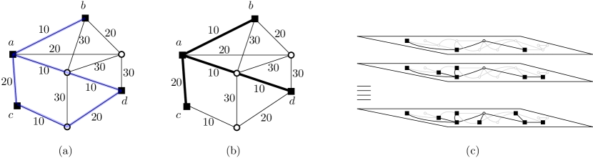
Real-life graphs can be very large, which motivates computing a subgraph that approximately preserves the shortest path distances among a subset of important vertices. Subsetwise spanner (also known as terminal spanners [15, 8]) is another commonly studied version, where in addition to , the input consists of a vertex subset of , known as terminals. The goal is to compute an additive or multiplicative spanner that guarantees that for every , is within an additive or multiplicative factor of . Computing a subsetwise spanner comes with additional challenges, e.g., consider computing a minimum spanning tree vs. a minimum Steiner tree for an analogy. There exist additive and additive subsetwise spanners with size and , respectively [3], however they do not come with any non-trivial lightness guarantees. The algorithms that construct such spanners often follow a greedy construction framework, i.e., they construct an initial graph and then examine the pairs in sorted nondecreasing order of the maximum weight, i.e., . For each pair , if it still fails to satisfy the distance condition of an additive spanner, then all the edges on the corresponding shortest path are added to the spanner.
In this paper, we focus on computing subsetwise additive spanners that are also light with respect to a Steiner tree . To this end, we define subset-lightness. Specifically, let be the pairs that do not satisfy the spanner condition in a minimum Steiner tree with terminal set . Let be a minimum Steiner tree with terminal set , where is the set of vertices on the shortest paths of the pairs in . Then, the subset-lightness is the ratio of the spanner weight to the weight of the minimum Steiner tree . Although it may initially appear that could be a simpler choice over when defining lightness for subsetwise spanners, may be a very loose lower bound. For example, consider a -vertex complete graph with vertex set and let be a partition of into equal-size subsets. Assume that the weight of each edge that is crossing the partition is and the weight of each remaining edge is , where . A minimum spanning tree of is a star graph with weight . Let be a graph obtained by subdividing each edge of once and distributing the weight of the edge equally among the two new edges. It is straightforward to verify that determines a minimum Steiner tree in with terminal set . Consider a pair , where , and the edge does not belong to . Then the weight of the shortest path in is and thus does not satisfy the distance condition for a spanner. There are pairs with one element in and the other in , and any +2 spanner must take all these shortest paths. Therefore, the ratio of a +2 spanner over the weight of would be very large, i.e., , whereas (i.e., a minimum Steiner tree with terminals ) is a better lower bound and gives a constant ratio. Therefore, we use to define subset-lightness.
The definition of subset-lightness naturally extends to the general case, i.e., when , where a minimum Steiner tree coincides with a minimum spanning tree. However, the techniques used to compute all-pairs additive spanners do not generalize to subsetwise additive spanners [2]. Therefore, a natural question is whether we can compute subsetwise spanners with non-trivial guarantees on subset-lightness, and in this paper, we answer this question affirmatively.
Our contribution. Let be a positive number, be a weighted graph and be a subset of vertices in . We show the following (also see Table 1).
-
1.
has a subsetwise spanner with subset-lightness (Theorem 2.1) and the spanner can be constructed deterministically.
-
2.
has a subsetwise spanner with subset-lightness (Theorem 2.2) and the spanner can be constructed deterministically.
-
3.
has a subsetwise spanner with subset-lightness, where is the maximum edge weight of the graph; and are the sets of vertices of the Steiner trees connecting and a randomly sampled subset of , respectively (Theorem 2.3).
| All-pairs Additive Spanners | Subsetwise Additive Spanners | ||||||
| Unweighted | Weighted | Weighted | |||||
| + | Lightness | Ref | + | Lightness | Ref | Subset-Lightness | Ref |
| 0 | [21] | + | [2] | Th 2.1 | |||
| +2 | [5, 22] | - | - | - | - | - | |
| +4 | [13] | +(4+ | [2] | , | Th 2.2, 2.3 | ||
| +6 | [9, 22] | - | - | - | - | - | |
Notice that the results of Theorem 2.1 and Theorem 2.2 exactly match the bounds provided for all-pairs spanners [2] if we set . Hence, our results are not only answering stronger questions, but they are also directly comparable with the existing results. The main challenge to generalizing the all-pairs results to subsetwise results is that the former compares against the minimum spanning tree. A counting argument that is often used in additive spanner constructions is based on the number of improvements, i.e., the number of improvements that may occur for all pairs of vertices is no more than an upper bound. Here, an improvement means that the difference in the shortest path between the pair before and after adding a set of edges is non-zero. However, this idea does not work in the subsetwise setting if we only compute a Steiner tree that spans . A key contribution of our work is that we address this problem by computing Steiner trees that not only span but also the vertices in the shortest paths of some vertex pairs from .
We next consider computing multi-level (multiplicative/additive) spanner, where the goal is to compute a hierarchy of (multiplicative/additive) spanners that minimizes the total number of edges or the total edge weight of all the spanners. Specifically, the input consists of a graph and some subsets of its vertices where . The goal is to find a hierarchy of spanners such that the spanner at the th level connects and for , the spanner includes the edges of the spanners . Multi-level spanners can model real-world scenarios where different levels of importance are assigned to different sets of vertices. Examples of such scenarios include modeling the quality of service requirements for the nodes in communication networks [12], or visualizing a graph on a map when the details are revealed as the users zoom in [20]. There exists a 4-approximation algorithm for this problem [4], and we give an improved -approximation (Theorem 3.1).
2 Lightweight Additive Subsetwise Spanner
In this section, we give our results on additive and lightweight spanners. All the spanners that we construct rely on the following preliminary setup.
2.1 Preliminary Setup
Let be a weighted graph and let be a set of given vertices. Fix a shortest path for each pair of vertices in . First, we compute a constant-factor approximation of the Steiner tree with as the set of terminals. Next, we identify the vertex pairs from for which the computed Steiner tree does not provide a path that satisfies the spanner condition. We then compute by taking the union of and the vertices from the shortest paths of those vertex pairs. To compute a lightweight subsetwise spanner of , we compute and , which are constant-factor approximations for the Steiner trees with terminal sets and , respectively. Note that an approximate Steiner tree can be computed in polynomial time [10]. We then construct a Steiner tree in with the set as terminals by taking the union of and and discarding unnecessary edges from . The reason for keeping the edges of is that later in our algorithm will use the vertices of , which we determined using . Since , we have , and hence . Therefore, we can compare asymptotic subset-lightness with respect to instead of . We will focus our attention on a weight-scaled version of and a subdivision of , which is described below.
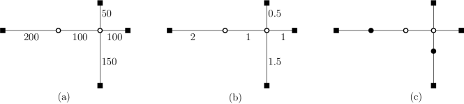
After computing , we multiply all edge weights of by to obtain a new weighted graph . Let be the scaled Steiner tree obtained from . We now observe some properties of that will be useful for the spanner construction. Although the Steiner tree has not been used previously for constructing lightweight spanners, such scaled graph has previously been used in [2] for constructing lightweight spanners. The following lemma shows this weight scaling preserves some distance relations.
Lemma 1
Let be a subgraph of and let be a subgraph of such that and (similarly, and ) correspond to the same set of vertices (edges) in . Then if and only if , where .
Proof
One can multiply to both sides of the inequality to obtain .
The following lemma shows that we can safely remove the edges of weight larger than from .
Lemma 2
Removal of the edges with weight larger than from does not increase the shortest path length for any pair of vertices of .
Proof
Assume for a contradiction that is an edge with weight larger than and removal of increases the shortest path length of . It now suffices to show that cannot be an edge on the shortest path between and . Note that the Steiner tree spans and . Therefore, the length of the shortest path between and in is at most the total edge weight of the scaled Steiner tree, i.e., multiplied by , which is equal to and hence the shortest path cannot contain .
We now construct a tree by subdividing the scaled Steiner tree , which will help extend techniques for spanner construction to guarantee subset-lightness (Figure 2). Specifically, we subdivide each edge of using a minimum number of subdivision vertices such that all edge weights in become less than or equal to one unit.
Lemma 3
Let be the number of subdivision vertices in . Then . and .
Proof
It suffices to subdivide each edge with vertices. The sum over all edges is bounded by . Since , we have .
2.2 A -spanner
Overview of the Construction. We construct the spanner incrementally by maintaining a current graph. We first take a set of Steiner tree edges (with as terminals) into the current graph and then examine each pair from in increasing order of . If the shortest path distance between in the current graph is more than what it requires for a -spanner, then we add all the edges on the shortest path between and in that are currently missing. During this step, we show that some pairs of vertices get ‘set-off’, i.e., their shortest path distances in the current graph become comparable to that of , and the number of such pairs is comparable to the total weight of the edges that have been added in this step. The final bound on the subset-lightness of the spanner comes by relating the total weight added to the total number of vertex pairs that were set off during the whole construction. A similar technique has previously been used to compute lightweight spanner for the whole graph, and using minimum spanning tree [2]. We extend that technique for subsetwise spanner using the Steiner tree.
Construction Details. For each vertex , let be the minimum weight edge incident to in . Let be a graph where and is obtained by choosing from all such edges the ones with a weight of less than one unit.
Lemma 4
Let be a shortest path in between a pair of vertices . Let be an edge of that does not belong to such that . Then there exists a vertex in such that .
Proof
Since , by construction, contains an edge incident to such that .
Lemma 5
The number of vertices of , and .
Proof
Since is a Steiner tree on terminal set , . Since for each vertex , we add at most one edge with weight less than one in , and .
Let be the graph obtained by adding all edges of and . The following claim shows that any edge in the shortest path in if does not exist in , then the end vertices of that edge has a close neighborhood (the set of neighbor vertices that has distance no more than the weight of the missing edge) in .
Lemma 6
Let be a shortest path in between a pair of vertices . Let be an edge of that does not belong to . Then there exists a set of vertices such that and for each vertex .
Proof
Note that and hence a vertex of . If , then the claim follows form Lemma 4 if we choose where is the neighbor of added in . Assume now that . By Lemma 2, and is obtained by subdividing the edges of such that the weight of each edge of becomes at most one. Since contains all edges of , we can set to be the set of vertices that has a distance less than or equal to in . Since the weight of edges of is at most 1, .
We are now ready to describe the algorithm. We create a graph by removing the edges from and adding the edges of . The algorithm sorts the pairs of vertices in based on their increasing order of maximum edge weight in the shortest path on . Then it checks whether the distance condition is unsatisfied for pairs of vertices in this sorted order, and if so then adds the missing edges on the corresponding shortest path. Specifically, let (initially, , which consists of all the edges of and ) be the current subgraph of . Then if the distance condition is unsatisfied, then the algorithm constructs by adding the missing edges of the shortest path to . Once all the unsatisfied pairs are processed, the spanner condition is satisfied for all pairs of vertices in . Although we used to check the spanner condition, where some edges may be subdivided, the subdivision does not change the shortest path length, and hence the final spanner corresponds to a valid spanner.

Lemma 7
Let be a subgraph of and let be the shortest path between and in . Let be the graph obtained from by adding the vertices and edges of that were missing in . Let be a vertex in and be a vertex in such that the distance where (see e.g., Figure 3(a)). If , where , where , then the following hold.
-
1.
and
-
2.
Either or .
Proof
Using triangle inequality, we have the following:
Similarly, we can show that . If and , then
However, we assumed . Hence either or .
By Lemma 7, at each step, the shortest path distances from and to a set of vertices (e.g., vertex in the lemma) in the current graph become comparable with their shortest path distances in . Such pairs are referred to as getting set-off. Furthermore, the shortest path distances in the current graph get smaller for some pair of vertices, e.g., or . We say either the pair or gets an improvement. We now show that a pair can only get improvements after its set-off.
Lemma 8
The total number of improvements of a pair of vertices after set-off is .
Proof
After the set-off of a particular pair , the shortest path distance between in the current graph is at most away from their shortest path distance in . Now each improvement decreases the shortest path distance of in the current graph by at least for some . Since the algorithm iterates in the increasing order of maximum edge weight on the shortest path in , the maximum number of improvements is .
Let be the spanner constructed above. We are now ready to bound its subset-lightness.
Theorem 2.1
The subset-lightness of the spanner is .
Proof
The weight of is less than or equal to . Hence the weight of is . In the next iterations, the algorithm adds missing edges of the shortest paths if the distance condition is unsatisfied. According to Lemma 6, for each missing edge added (on the shortest path ) there is a neighborhood of size equal to the weight of the missing edge. Let us assume that the total weight of the missing edges is . We claim a neighborhood of size . For the sake of contradiction let us assume that the neighborhood has size . But then we have a shorter path than the shortest path , a contradiction.
According to Lemma 7, each vertex in this -size neighborhood gets set-off or improvement. Hence the total edge weight added in the remaining iterations is equal to the total number of set-offs and improvements of vertex pairs from . Since , the number such vertex pairs is . Each of these pairs gets at most one set-off and improvements after set-off. Hence the total count is . Assuming and are constants, the total spanner weight is , where .
Note that the subset-lightness bound in Theorem 2.1 is tight because for a complete graph with edges of unit weight and equal to the vertex set, any spanner, where , gets edges and thus a subset-lightness of .
2.3 A -spanner
Some initial steps of our -spanner construction are the same as our -spanner construction, i.e., we construct the graphs , , , and . The construction of differs from that in the -spanner construction; in the -spanner construction, the vertex set of is and we add at most one edge incident to each vertex in . In our -spanner, to construct , we sort all the neighbors of in according to the increasing order of edge weights for each vertex . We add edges to until the total weight of edges added adjacent to is no more than (where is a parameter we will optimize later). We then construct by adding the edges of and .
Lemma 9
Let be a shortest path in between a pair of vertices . Let be an edge of that does not belong to . Then there exists a set of vertices such that and for each vertex .
Proof
If the weight of is no more than , then since is a missing edge we added at least neighbors of in . Let be those neighbors and then satisfies the desired property. Assume now that . By Lemma 2, and is obtained by subdividing the edges of such that the weight of each edge of becomes at most one. Since contains all edges of , we can set to be the set of vertices that has a distance less than or equal to in . Since the weight of edges of is at most 1, .
We then iteratively consider the shortest paths between pairs of vertices of and for the pairs that do not satisfy the distance condition, we add edges (that are missing on the shortest path) to the current graph . However, since we allow for a larger distance bound for -spanners, our goal is to show that a larger number of pairs of vertices of gets set off at each iteration. The following lemma would help achieve this goal.
Lemma 10
Let be a subgraph of and let be the shortest path between and in . Let be the graph obtained from by adding the vertices and edges of that were missing in . Let be a vertex in and be a vertex such that the distance where . Let and be two vertices such that and , respectively (see e.g., Figure 3(b)). If , where and , then the following hold.
-
1.
and .
-
2.
Either or .
Proof
Using triangle inequality, we can show the following:
Similarly, we can show that . If and , then
However, we assumed . Hence either or .
After computing and , our algorithm sorts the pairs of vertices in based on their increasing order of maximum edge weight in the shortest path on ; If multiple pairs have the same maximum edge weight, then the algorithm selects the pair with the smaller shortest path length. Then it checks whether the spanner condition is unsatisfied for pairs of vertices according to the sorted order. Let be the current subgraph of . If the condition is unsatisfied, then the algorithm computes by adding the missing edges at of the shortest path of the unsatisfied pair at . Once all the unsatisfied pairs are considered, we have a valid spanner. By Lemma 10, at each iteration, the shortest path distances from close neighbors of and to a set of other vertices become comparable with the shortest path distance of , where are the vertices being considered in that iteration. In other words, for each vertex pairs and satisfying the conditions of the lemma, and . We say that the pairs and get set-off when the shortest paths of the pairs become comparable with respect to the shortest path in for the first time. Also, according to the lemma, the shortest paths get smaller either for or for : or . We say either the pair or gets an improvement. Similar to Lemma 8, we can show the total number of improvements of a pair after set-off is .
Theorem 2.2
The subset-lightness of the spanner is .
Proof
By the construction of , . In the next iterations, the algorithm adds missing edges of the shortest paths if the distance condition is unsatisfied. According to Lemma 6, for each missing edge added, there is a neighborhood of size equal to the weight of the missing edge. According to Lemma 10, each vertex pair formed from these neighborhoods and the neighborhoods of the endpoints of the shortest path get set-off or improvements. Let the missing edges of the shortest path between be added when we construct from . Let and be the shortest path edges. Notice that, neither nor are present in , otherwise the algorithm would not select the pair (and we would select the pair since their shortest path is shorter). According to Lemma 9, there are vertices that form a pair with the neighborhood of size equal to weight of missing edges in the shortest path such that each of these pairs are either get set-off or improvements. Hence there are at least improvements where is the total weights added in the iterations of the algorithms after constructing . On the other hand, the size of the set of vertex pairs that can get set-off or improvements is . Each of these pairs gets at most one set-off and improvements after set-off. If we set up , then . Hence the total weight of the spanner is . If we set , then the total weight of the spanner is . Hence, the subset-lightness of this spanner is .
2.4 A Sampling-based -spanner
The initial steps of this algorithm are similar to the previous algorithm. We first compute the Steiner tree , scaled graph , subdivided tree , initial graph , add to to achieve , subdivide Steiner tree edges in the input graph to achieve . We now consider each pair of vertices . Let be the shortest path between in . Let be the total weight of missing edges in considering the edges of . If , we then add all the missing edges where is a parameter we will set later. The total weight added in this step is no more than .
To handle vertex pairs with , we consider the subpath in at the beginning of that has missing edges of weight . We refer to that subpath as the prefix and similarly, we define the suffix. We then uniformly sample vertices from where is a small constant. We also add the missing edges of prefixes and suffixes. If the prefix and suffix overlap, we then add all the missing edges of the shortest path; otherwise, both prefix and suffix have a neighborhood of size . Now the probability that the sampled vertices will not hit the neighborhood of suffix and prefix is equal to . Hence with a high probability, the sampled vertices will hit the neighborhood of the suffix and prefix.
We then compute a -spanner on the sampled vertices and add the spanner edges in . We can show that we will achieve a valid -spanner with high probability. Consider a vertex pair for which we haven’t added all the missing edges. Let be two vertices in the prefix and suffix of respectively, such that sampled vertices hit their neighborhood. Let and be the corresponding neighbor vertices of and respectively. Then
The weight of -spanner on sampled vertices can be computed using Theorem 2.1. Let be the Steiner tree spanning the shortest path vertices of the sampled vertices. Then the weight of the -spanner is . Hence the total edge weight of is . If we set , then is . Hence the subset-lightness of the spanner is . Notice that we can not assume that is arbitrarily small since it depends on . We can run a binary search on and select an that is approximately . If we don’t find such an we can compute a -spanner on .
Theorem 2.3
The subset-lightness of the spanner is .
3 Multi-Level Spanners
In this section, we study a generalization of the subsetwise spanner problem. We now have a hierarchy of vertex subsets where . For each level , we compute a (multiplicative or additive) subsetwise spanner where the edge sets of these spanners are also nested, e.g., . This problem is called the multi-level spanner problem. We provide an -approximation algorithm for the multi-level spanner problem which is better than the existing -approximation [4].
The existing -approximation is achieved by first generating a rounding-up instance where each subset is rounded up to a level that is the nearest power of 2, e.g., . Then a spanner is computed independently for each rounded-up level and merged together to achieve a spanner for the edge level. The merging step provides a feasible solution that is a -approximation of the rounded-up instance. On the other hand, the rounding-up step can increase the cost by at most two times the input instance. Overall, the algorithm is thus a -approximation.
We generalize this algorithm by introducing two parameters, and . Instead of starting from level , we start from level ; and instead of considering the levels , we consider the levels for rounding up. Our algorithm is randomized, and we show the expected cost of the output with respect to . We then select the best value of to achieve the desired approximation ratio of the algorithm.
Our approach has two main steps: the first step rounds up the level of all terminals to a level equal to where , , and is a nonnegative integer; the second step computes a solution independently for each rounded-up level and merges all solutions from the highest level to the lowest level. We show that the first step can make the solution at most times worse than the optimal solution, and the second step can make the solution at most times worse than the optimal solution. By optimizing , we achieve an -approximation algorithm. We provide the pseudocode of the algorithm below, here is the largest integer such that .
The cost of the multi-level solution may increase due to rounding up and the merging steps. The following results provide the costs of these steps.
Lemma 11
The expected rounding cost is .
Proof
Assume that the highest level of a particular edge is equal to before rounding. Since , after rounding we will face one of two cases; case 1: , the highest level of the edge becomes and case 2: , the highest level of the edge becomes . Since the lowest level is and , the expected ratio to rounding cost and optimal cost is: .
We now establish an upper bound for the merging step. We show that this upper bound depends only on , regardless of the value of .
Lemma 12
If we compute independent solutions of a rounded-up instance and merge them, then the cost of the solution is no more than .
Proof
Assume that . Let the rounded-up terminal subsets be . Suppose we have computed the independent solution and merged them in lower levels. Note that in the worst case the cost of approximation algorithm is , and cost of the optimal algorithm is . We show that . We provide a proof by induction on .
If , then we have just one terminal subset . The approximation algorithm computes a spanner for and there is nothing to merge. Since the approximation algorithm uses an optimal algorithm to compute independent solutions, weight() weight() weight() since .
We now assume that the claim is true for which is the induction hypothesis. Hence . We now show that the claim is also true for . In other words, we show that , using the facts that an independent optimal solution has a cost lower than or equal to any other solution, and that the input is a rounded up instance.
Let . Let the rounded-up terminal subsets be . Suppose we have computed the independent solution and merged them in lower levels. We actually prove a stronger claim, and use that to prove the lemma. Note that in the worst case the cost of approximation algorithm is . And the cost of the optimal algorithm is . We show that . We provide a proof by induction on .
Base step: If , then we have just one terminal subset . The approximation algorithm computes a spanner for and there is nothing to merge. Since the approximation algorithm uses an optimal algorithm to compute independent solutions, weight() weight() weight() since .
Inductive step: We assume that the claim is true for which is the induction hypothesis. Hence . We now show that the claim is also true for . In other words, we have to show that . We know,
Here, the second equality is just a simplification. The third inequality uses the fact that an independent optimal solution has a cost lower than or equal to any other solution. The fourth equality is a simplification, the fifth inequality uses the fact that the input is a rounded up instance. The sixth inequality uses the induction hypothesis.
Lemma 11 and Lemma 12 show that Algorithm -level approximation provides a multi-level spanner with cost no more than . The minimum value of is when we put .
Theorem 3.1
Algorithm -level approximation computes a -level spanner with expected weight at most .
4 Conclusion
We designed subsetwise and spanners with and subset-lightness guarantees, respectively. Both spanners can be constructed deterministically. Using a sampling technique we provided the construction for a subsetwise spanner. We also gave an -approximation algorithms for computing multi-level spanners. It would be interesting if the subset-lightness bound of our subsetwise spanners can be reduced to sublinear bounds, even for some specific graph classes.
References
- [1] Amir Abboud and Greg Bodwin. The 4/3 additive spanner exponent is tight, 2015.
- [2] Reyan Ahmed, Greg Bodwin, Keaton Hamm, Stephen Kobourov, and Richard Spence. On additive spanners in weighted graphs with local error. In 47th International Workshop on Graph-Theoretic Concepts in Computer Science (WG), pages 361–373. Springer, 2021.
- [3] Reyan Ahmed, Greg Bodwin, Faryad Darabi Sahneh, Keaton Hamm, Mohammad Javad Latifi Jebelli, Stephen Kobourov, and Richard Spence. Graph spanners: A tutorial review. Computer Science Review, 37:100253, 2020.
- [4] Reyan Ahmed, Keaton Hamm, Stephen Kobourov, Mohammad Javad Latifi Jebelli, Faryad Darabi Sahneh, and Richard Spence. Multi-priority graph sparsification. In International Workshop on Combinatorial Algorithms, pages 1–12. Springer, 2023.
- [5] Donald Aingworth, Chandra Chekuri, Piotr Indyk, and Rajeev Motwani. Fast estimation of diameter and shortest paths (without matrix multiplication). SIAM Journal on Computing, 28:1167–1181, 1999.
- [6] Ingo Althöfer, Gautam Das, David Dobkin, and Deborah Joseph. Generating sparse spanners for weighted graphs. In Scandinavian Workshop on Algorithm Theory (SWAT), pages 26–37, Berlin, Heidelberg, 1990. Springer Berlin Heidelberg.
- [7] Baruch Awerbuch. Complexity of network synchronization. Journal of the ACM (JACM), 32(4):804–823, 1985.
- [8] Yair Bartal, Arnold Filtser, and Ofer Neiman. On notions of distortion and an almost minimum spanning tree with constant average distortion. Journal of Computer and System Sciences, 105:116–129, 2019.
- [9] Surender Baswana, Telikepalli Kavitha, Kurt Mehlhorn, and Seth Pettie. Additive spanners and (, )-spanners. ACM Transactions on Algorithms (TALG), 7(1):5, 2010.
- [10] Jaroslaw Byrka, Fabrizio Grandoni, Thomas Rothvoß, and Laura Sanità. Steiner tree approximation via iterative randomized rounding. J. ACM, 60(1):6:1–6:33, 2013.
- [11] Barun Chandra, Gautam Das, Giri Narasimhan, and José Soares. New sparseness results on graph spanners. In Proceedings of the eighth annual symposium on Computational geometry, pages 192–201. ACM, 1992.
- [12] M. Charikar, J. Naor, and B. Schieber. Resource optimization in QoS multicast routing of real-time multimedia. IEEE/ACM Transactions on Networking, 12(2):340–348, April 2004.
- [13] Shiri Chechik. New additive spanners. In Proceedings of the Twenty-Fourth Annual ACM-SIAM Symposium on Discrete Algorithms (SODA), pages 498–512. Society for Industrial and Applied Mathematics, 2013.
- [14] Shiri Chechik and Christian Wulff-Nilsen. Near-optimal light spanners. ACM Transactions on Algorithms (TALG), 14(3):1–15, 2018.
- [15] Michael Elkin, Arnold Filtser, and Ofer Neiman. Terminal embeddings. Theoretical Computer Science, 697:1–36, 2017.
- [16] Michael Elkin, Yuval Gitlitz, and Ofer Neiman. Almost shortest paths and PRAM distance oracles in weighted graphs. arXiv preprint arXiv:1907.11422, 2019.
- [17] Michael Elkin, Yuval Gitlitz, and Ofer Neiman. Improved weighted additive spanners. Distributed Computing, 36(3):385–394, 2023.
- [18] Michael Elkin, Ofer Neiman, and Shay Solomon. Light spanners. In International Colloquium on Automata, Languages, and Programming, pages 442–452. Springer, 2014.
- [19] Arnold Filtser and Shay Solomon. The greedy spanner is existentially optimal. SIAM Journal on Computing, 49(2):429–447, 2020.
- [20] Kathryn Gray, Mingwei Li, Reyan Ahmed, Md Khaledur Rahman, Ariful Azad, Stephen Kobourov, and Katy Börner. A scalable method for readable tree layouts. IEEE Transactions on Visualization and Computer Graphics, 2023.
- [21] Samir Khuller, Balaji Raghavachari, and Neal Young. Balancing minimum spanning trees and shortest-path trees. Algorithmica, 14(4):305–321, 1995.
- [22] Mathias Bæk Tejs Knudsen. Additive spanners: A simple construction. In Scandinavian Workshop on Algorithm Theory (SWAT), pages 277–281. Springer, 2014.
- [23] G. Kortsarz. On the hardness of approximating spanners. Algorithmica, 30(3):432–450, Jan 2001.
- [24] Hung Le and Shay Solomon. A unified framework for light spanners. In Proceedings of the 55th Annual ACM Symposium on Theory of Computing, pages 295–308, 2023.
- [25] Arthur L Liestman and Thomas C Shermer. Additive graph spanners. Networks, 23(4):343–363, 1993.
- [26] David Peleg and Alejandro A Schäffer. Graph spanners. Journal of graph theory, 13(1):99–116, 1989.